Combined analytical and numerical approach to study magnetization plateaux in doped quasi-one-dimensional antiferromagnets

Abstract

We investigate the magnetic properties of quasi one-dimensional quantum spin-$S$ antiferromagnets. We use a combination of analytical and numerical techniques to study the presence of plateaux in the magnetization curve. The analytical technique consists in a path integral formulation in terms of coherent states. This technique can be extended to the presence of doping and has the advantage of a much better control for large spins than the usual bosonization technique. We discuss the appearance of doping-dependent plateaux in the magnetization curves for spin-$S$ chains and ladders. The analytical results are complemented by a Density matrix Renormalization Group (DMRG) study for a trimerized spin-$1/2$ and anisotropic spin-$3/2$ doped chains.

I Introduction

One-dimensional and quasi one-dimensional quantum spin systems have been a subject of close attention in condensed matter physics. Over the past decades, much progress has emerged from the studies of such low-dimensional systems, the Haldane gap Haldane and the magnetization plateaux OYA ; plateaux_ladd ; Plateaux_pmer being some of the best-known examples. In particular, spin chains have allowed to study quantum magnetism in the simplest tractable setting, while investigations of spin ladders have permitted first steps in the study of crossover from one to two dimensions.

The present work is devoted to magnetization plateaux in quantum antiferromagnets: the magnetization remaining spectacularly constant in a finite interval of external magnetic field. This phenomenon has been found in a great variety of systems from spin ladders plateaux_ladd and $p$-merized chains Plateaux_pmer to frustrated higher dimensional systems. penc .

For a quantum spin-$S$ chain, the necessary condition for the occurrence of a magnetization plateau has been established by Oshikawa, Yamanaka and Affleck OYA :

$$N(S-m)\in\mathbb{Z},$$ (1)

where $m$ is the magnetization per site, $N$ is the number of spins per unit cell, and $\mathbb{Z}$ is the set of all integers.

This condition restricts the plateau magnetization $m$ to rational values. However, it has been argued that plateaux may also appear at an irrational $m$, as a result of either quenched disorder Plateau_disorder or doping with itinerant carriers Cabra_irrational ; Poilblanc2004 ; Roux_irrational ; Roux_2007 ; Roux_PhD . In the latter case, doping may allow to reduce the $m$ in a controlled way, thus making the plateau more easily accessible to experiments in lower magnetic fields.

Unfortunately, the analytical methods, used so far to study magnetization plateaux in spin chains and ladders, have been limited to bosonization (and thus, effectively, to one-dimensional spin-$1/2$ systems) – and to the bond operator technique, intrinsically restricted to spin-$1/2$ systems MomTot . However, recently, Tanaka, Totsuka and Hu Tanaka (TTH) have arrived at the necessary condition of Ref. OYA, using the Haldane’s path integral approach. This approach is applicable regardless of the dimensionality or of the value $S$ of the spin – and, below, we explore how much progress it may afford us in understanding the magnetization plateaux in various systems from spin-$1/2$ chains to higer-spin systems. This approach open new perspectives in understanding the physics of magnetization plateaux in higher spin and higher dimensional systems such as rare earth tetraborides RET .

Our goal in this paper is to test and extend the approach developed by Tanaka et al.Tanaka . First, we test the technique on several concrete small-spin $N$-leg ladders and $p$-merized chains, previously studied with the help of bosonization plateaux_ladd ; Plateaux_pmer . Then we extend the technique by combining it with ideas due to R. Shankar Shankar , to account for hole doping in spin chains at non-zero magnetization. Unfortunately, accounting for hole doping in zero field has proven to be problematic for technical reasons which we are not going to discuss here. However, at a non-zero average magnetization per site the technical difficulties are lifted, which allows us to generalize the TTH approach to the case of doping. After this, we use doped Hubbard and $t-J$ chains and ladders as a testing ground, and re-derive some of the results previously found for these systems Cabra_irrational ; Poilblanc2004 ; Roux_irrational ; Roux_2007 . Then, we turn to doped higher-spin systems, which tend to pose a problem for the bosonization approach.

In Section II, we illustrate the key points of Ref. Tanaka, by studying magnetization plateaux in an anisotropic spin chain with the help of coherent-state path integral technique. In Section III, we extend this to a dimerized chain, and to a two-leg spin ladder – and then, in section IV, we generalize the above to $n$-leg ladders and $p$-merized chains, and find that they satisfy the necessary condition of the Eq. (1).

In Section V, we generalize the plateau condition in the Eq. (1) to account for the doping dependence. In a spin-$S$ system at a small hole density $\delta\ll 1$, we find the plateau condition to read

$$N\left(1-\frac{\delta}{2S}\right)(S\pm m)\in\mathbb{Z}.$$ (2)

The Section VI presents an application of the formalism to a doped spin-$3/2$ chain, and compares the results with those obtained numerically by DMRG.

In Section VII, we discuss the plateau condition for a doped $n$-leg ladders and $p$-merized chains, with and without doping.

In Section VIII, we present the results for a trimerized chain, and compare with DMRG results.

Finally, in Section IX we present the conclusions, possible implications and extensions of the present approach to higher dimensions.

II Anisotropic spin chain in a magnetic field

In this Section, we study the spin-$S$ nearest-neighbor antiferromagnetic (AF) chain with easy-plane single-ion anisotropy, subject to a transverse magnetic field:

$$H=J\sum_{j}\vec{\mathbf{S}}_{j}\cdot\vec{\mathbf{S}}_{j+1}+D\sum_{j}(\mathbf{S}^{z}_{j})^{2}-h\sum_{j}\mathbf{S}^{z}_{j},$$ (3)

where $J$ is positive, and the magnetic field $h$ points in the $z$ direction, as shown in the Fig. 1.

Following the Ref. Tanaka, , we analyze the system using the coherent-state path integral description due to Haldane Haldane . The resulting effective action comprises two terms: the first one is the coherent-state expectation value of the Hamiltonian, and the second one, dubbed the Berry phase term, corresponds to the solid angle swept by the spins in their imaginary time evolution.

In order to obtain an effective theory, first, we identify the classical ground-state configuration and the low-energy modes above it. Partially polarized by the magnetic field, the spins form a canted texture, that we parametrize as $\vec{S}_{j}=S\vec{n}_{j}$, with $\vec{n}_{j}$ being a unit vector with staggered XY components ($\phi_{j}=\frac{\pi}{a}x_{j}$):

$$\vec{S}_{j}=\left(S\sin{\theta_{j}}\;\cos{\phi_{j}},S\sin{\theta_{j}}\;\sin{\phi_{j}},S\cos{\theta_{j}}\right).$$ (4)

We parametrize the fluctuations around the above canted state as per

$$\phi_{j}\rightarrow\frac{\pi}{a}x_{j}+\phi(x_{j})\hskip 28.45274pt\theta_{j}\rightarrow\theta_{0}+\delta\theta(x_{j}),$$ (5)

where $\theta_{0}$ is the classical ground state solution $\cos{\theta_{0}}=\frac{h}{2S(2J+D)}$ and $x_{j}=aj$, with $a$ the lattice constant.

Expanding up to the second order in the $\delta\theta$, we can write $S^{\pm}_{j}=S^{x}_{j}\pm iS^{y}_{j}$ as a function of $\delta\theta(x_{j})$ and $\phi(x_{j})$ and, using these fluctuation fields, we write an effective theory. If we calculate the Poisson Brackets $\{S^{z},S^{\pm}\}_{\phi,\delta\theta}$, we obtain $i\hbar\{S^{z},S^{\pm}\}_{\phi,\delta\theta}=-S(\sin{\theta_{0}}-\delta\theta\cos{\theta_{0}})\left(\pm\hbar S^{\pm}\right)$ then is straightforward to see that defining

$$a\Pi(x_{j})=-S\left[\delta\theta(x_{j})\sin{\theta_{0}}+\frac{1}{2}(\delta\theta(x_{j}))^{2}\cos{\theta_{0}}\right]$$ (6)

as the conjugate field of $\phi$ we have the correct commutation relations for the spin operators

$$S^{z}_{j} \simeq S\cos{\theta_{0}}+a\Pi(x_{j})$$ (7)

$$S^{\pm}_{j} \simeq (-1)^{j}e^{\pm i\phi(x_{j})}\left[S\sin{\theta_{0}}-\frac{a\,m}{S\sin{\theta_{0}}}\Pi(x_{j})\right.$$

$$- \left.\frac{a^{2}}{2}\frac{S^{2}}{S^{2}-m^{2}}\frac{1}{S\sin{\theta_{0}}}\Pi^{2}(x_{j})\right],$$

where $m=S\cos{\theta_{0}}$.

Figure 1: Classical configuration for a spin chain in the presence of a magnetic field.

Following the Ref. Tanaka, , one arrives at the low-energy continuous effective action, corresponding to the Hamiltonian (3):

$$S\!\! = \!\!\!\int\!dxd\tau\left\{a\left(2J+D\right)\Pi^{2}\!-\!i(\partial_{\tau}\phi)\Pi\right.$$ (9)

$$+ \left.\frac{J}{2}a(S^{2}-m^{2})(\partial_{x}\phi)^{2}+i\left(\frac{S-m}{a}\right)(\partial_{\tau}\phi)\right\}.$$

The last term in right hand side of the Eq. (9) arises from the Berry phase of the individual spins in the Eq. (3). After gaussian integration over the field $\Pi$, the action (9) takes the form

$$S\!=\!\!\int dxd\tau\left\{\frac{K_{\tau}}{2}(\partial_{\tau}\phi)^{2}\!+\!\frac{K_{x}}{2}(\partial_{x}\phi)^{2}\!+\!i\left(\!\frac{S-m}{a}\!\right)\!(\partial_{\tau}\phi)\right\}$$

(10)

with

$$K_{\tau}=\frac{1}{2a\left(2J+D\right)}\hskip 28.45274ptK_{x}=Ja(S^{2}-m^{2}).$$ (11)

The last term in (10) counts the winding number of the space-time history of the field $\phi$, defined on a covering space of a circle. In order to understand the consequences of the topological term, it is convenient to apply a standard duality transformation to the action. First, the phase field $\phi$ is written as $\phi=\phi_{v}+\phi_{t}$, where $\phi_{v}$ is a fixed field configuration containing all the vortices $(\partial_{\mu}\partial_{\nu}-\partial_{\nu}\partial_{\mu})\phi_{v}\neq 0$, and $\phi_{t}$ contains the fluctuating vortex-free part. Next, we introduce the Hubbard-Stratonovich auxiliary vector field $J_{\mu}=(J_{\tau},J_{x})$, and integrating by parts we obtain

$$S = \int dxd\tau\left\{\phantom{\frac{1}{2}}i\left(J_{\tau}+\left(\frac{S-m}{a}\right)\right)(\partial_{\tau}\phi_{v})\right.$$

$$+ iJ_{x}(\partial_{x}\phi_{v})+\frac{1}{2}\frac{J^{2}_{\tau}}{K_{\tau}}+\left.\frac{1}{2}\frac{J^{2}_{x}}{K_{x}}\right.$$

$$- \left.i\left[\partial_{\tau}\left(J_{\tau}+\left(\frac{S-m}{a}\right)\right)+\partial_{x}J_{x}\right]\phi_{t}\phantom{\frac{1}{2}}\right\}.$$

Defining $\tilde{J}_{\mu}=J_{\mu}+\delta_{\mu,0}\left(\frac{S-m}{a}\right)$ the vorticity-free part can be eliminated with the constraint $\partial_{\mu}\tilde{J}_{\mu}=0$. Then, the action reads

$$S=\int\!dxd\tau\left\{i\tilde{J}_{\mu}\partial_{\mu}\phi_{v}+\frac{1}{2K_{\tau}}\left(\tilde{J}_{\mu}-\left(\frac{S-m}{a}\right)\right)^{2}\!\!+\frac{1}{2K_{x}}\tilde{J}^{2}_{x}\right\}.$$

The constraint $\partial_{\mu}\tilde{J}_{\mu}=0$ is solved in one dimension (1D) in terms of an auxiliary field by

$$\tilde{J}_{\mu}=\epsilon_{\mu\nu}\partial_{\nu}\chi,$$ (13)

where $\chi$ is vorticity-free. Integrating the first term in the action by parts, and using the substitution $\chi\rightarrow\tilde{\chi}+\left(\frac{S-m}{a}\right)x$, we obtain

$$S = \int dxd\tau\left\{\frac{1}{2K_{\tau}}(\partial_{x}\tilde{\chi})^{2}+\frac{1}{2K_{x}}(\partial_{\tau}\tilde{\chi})^{2}\right.$$ (14)

$$+ \left.iB\left(\tilde{\chi}+\left(\frac{S-m}{a}\right)x\right)\right\},$$

where $B=\epsilon_{\mu\nu}\partial_{\mu}\partial_{\nu}\phi_{v}=\sum_{j}2\pi q_{j}\delta(\tau-\tilde{\tau}_{j})\delta(x-\tilde{x}_{j})$. Here, $\tilde{\tau}_{j}$ and $\tilde{x}_{j}$ are the time and space coordinates of the $j$-th vortex event and $q_{j}$ is the vorticity. Upon summation over the vortex configurations in the partition function, and then rescaling the time variable, the action is brought to the form

$$S = \int dxd\tau\left\{\phantom{\frac{1}{2}}\frac{1}{2\sqrt{K_{\tau}K_{x}}}\left((\partial_{x}\tilde{\chi})^{2}+(\partial_{\tau}\tilde{\chi})^{2}\right)\right.$$ (15)

$$+ \left.\tilde{\lambda}_{1}\cos{\left(2\pi\left(\tilde{\chi}+\left(\frac{S-m}{a}\right)x\right)\right)}\phantom{\frac{1}{2}}\right\}.$$

This effective action is identical to the one obtained in the Ref. OYA, via bosonization. The cosine term is commensurate for $S-m\in\mathbb{Z}$. The magnetic excitations are gapless for all the values of $m$ that satisfy $S-m\notin\mathbb{Z}$. Then, when the condition

$$S-m\in\mathbb{Z}$$ (16)

is satisfied, a plateau can occur for some range of parameters if the scaling dimension of the perturbation is small enough. More precisely, the presence of the cosine operator in the Eq. (15) is not enough to produce a gap in the spectrum. The stiffness of the $\tilde{\chi}$ field must be such that this operator has scaling $d$ dimension smaller than $2$. Since $d$ is a decreasing function of $D$, we expect a plateau for large enough values of this parameter.

The condition (16) is the well-known result of Oshikawa, Yamanaka and Affleck OYA , which generalizes the argument due to Lieb, Schulz and MattisLSM .

A more general situation arises when $S-m=p/r$, with $p,r\in\mathbb{Z}$. In this case, the vortices whose winding numbers are integer multiples of $r$ are free of destructive interference. In this case, only vortices with vorticity $\pm r$ are able to condense. In the effective action, this is signalled by the $r$th harmonic of the cosine term in the harmonic expansion being commensurate. If relevant, this cosine operator gives rise to a gapped $r$-fold degenerate ground state and fractionalized excitations Tanaka . The best-known example of such a scenario is the AF chain with a strong enough second-neighbor AF couplingokunishi . The system is then in a gapped phase with two degenerate spontaneously dimerized ground states; fractional excitations are spinons – domain walls between these two ground states. In what follows, we concentrate on the case $S-m\in\mathbb{Z}$.

At this point, we would like to make an observation, which will prove useful in the Section V, when comparing the plateau condition for doped systems with that at zero doping: According to the Eq. (10), for each contribution to the partition function, the Berry phase term provides a weight factor

$$e^{i(S-m)\sum_{j}\int d\tau\partial_{\tau}\phi_{j}},$$

where the integral $\int d\tau\partial_{\tau}\phi_{j}=2\pi n_{j}$ is an integer times $2\pi$, and the subscript $j$ labels the spins in the chain. Inverting the sign in front of the $S$ changes the imaginary exponent by $4\pi n_{j}S$, which is an integer times $2\pi$ both for integer and half-integer $S$. Therefore, the necessary condition (16) for the magnetization plateau may be equivalently presented as

$$(S\pm m)\in\mathbb{Z}.$$ (17)

In the following, we would like to extend the approach above to other one-dimensional spin systems. In the next section, we discuss the cases of a two-leg ladder and a dimerized spin chain. Then, in the Section V, we study the magnetization plateaux in the presence of doping.

III Two-leg ladders and dimerized chains

III.1 Two-leg spin ladder

The formalism above can be used to study more involved spin models, such as spin ladders, that interpolate between one and two dimensions. For spin $1/2$ experimental evidence of zero magnetization plateaux has been reported for instance in (C₅H₁₂N)₂CuBr₄ Watson_2001 . In this section we study two-leg ladders with single-ion anisotropy in a magnetic field, and in the next section we discuss extensions to $N$-leg ladders and $p$-merized chains.

Consider the following Hamiltonian

$$H = \sum_{j}\left\{J_{\shortparallel}(\vec{\mathbf{S}}_{1,j}\cdot\vec{\mathbf{S}}_{1,j+1}+\vec{\mathbf{S}}_{2,j}\cdot\vec{\mathbf{S}}_{2,j+1})\right.$$

$$+ \left.J_{\bot}\vec{\mathbf{S}}_{1,j}\cdot\vec{\mathbf{S}}_{2,j}+D((\mathbf{S}^{z}_{1,j})^{2}+(\mathbf{S}^{z}_{2,j})^{2})\right.$$

$$- \left.h((\mathbf{S}^{z}_{1,j})+(\mathbf{S}^{z}_{2,j}))\right\},$$

where $J_{\shortparallel}$ is the antiferromagnetic coupling along the chain, and $J_{\bot}$ is the inter-chain coupling. The onsite anisotropy term is added only for completeness and we can recover the isotropic case by taking the $D=0$ limit.

In the $S\rightarrow\infty$ limit we can write the energy of the system as a function of the angle $\theta$ (see Fig. 2), with the minimum at

$$\cos{\theta_{0}}=\frac{h}{2S(2J_{\shortparallel}+J_{\bot}+D)}.$$ (19)

As before, we parametrize the fluctuations in terms of the fields $\delta\theta_{\alpha}$ and $\phi_{\alpha}$, where $\alpha=1,2$ is the chain index. Equations (6), (7) and (II) have the same form in each chain. Using this parametrization in the Hamiltonian, retaining terms up to second order in the fields and switching to the path integral language, we obtain the action

$$S\! = \!\int dxd\tau\left\{\frac{J_{\shortparallel}}{2}a(S^{2}-m^{2})((\partial_{x}\phi_{1})^{2}+(\partial_{x}\phi_{2})^{2})\right.$$

$$+ \!\left.\frac{J_{\bot}}{2}\!\left(\frac{S^{2}\!-\!m^{2}}{a}\right)\!(\phi_{2}\!-\!\phi_{1})^{2}\!+\!i\left(\frac{S\!-\!m}{a}\right)\partial_{\tau}(\phi_{1}+\phi_{2})\right\}$$

$$+ \!\int dxd\tau\left\{a\left(2J_{\shortparallel}+J_{\bot}\frac{S^{2}}{S^{2}-m^{2}}+D\right)\left(\Pi_{1}^{2}+\Pi_{2}^{2}\right)\right.$$

$$+ \!\!\left.J_{\bot}a\left(1-\frac{m^{2}}{S^{2}-m^{2}}\right)\Pi_{1}\Pi_{2}-i\left(\Pi_{1}\partial_{\tau}\phi_{1}+\Pi_{2}\partial_{\tau}\phi_{2}\right)\right\}.$$

Integrating over the $\Pi$-fields and using the transformation $\vec{\varphi}=U\vec{\phi}$ with

$$\vec{\varphi}=\left(\begin{array}[]{c}\varphi_{a}\\ \varphi_{s}\end{array}\right)\hskip 14.22636pt\vec{\phi}=\left(\begin{array}[]{c}\phi_{1}\\ \phi_{2}\end{array}\right)\hskip 14.22636ptU=\left(\begin{array}[]{cc}1&-1\\ \frac{1}{2}&\frac{1}{2}\end{array}\right)$$ (27)

we can write $S=S_{s}+S_{a}$, with

$$S_{s} = \int d\tau dx\left\{\frac{1}{2}K_{x}^{(s)}(\partial_{x}\varphi_{s})^{2}+\frac{1}{2}K_{\tau}^{(s)}(\partial_{\tau}\varphi_{s})^{2}\right.$$

$$+ \left.i\;2\left(\frac{S-m}{a}\right)(\partial_{\tau}\varphi_{s})\right\}$$

and

$$S_{a} = \int dxd\tau\left\{\frac{1}{2}K_{x}^{(a)}(\partial_{x}\varphi_{a})^{2}+\frac{1}{2}K_{\tau}^{(a)}(\partial_{\tau}\varphi_{a})^{2}\right.$$

$$+ \left.2J_{\bot}\left(\frac{S^{2}-m^{2}}{a}\right)\varphi_{a}^{2}\right\},$$

where

$$K_{x}^{(a)} = K_{x}^{(s)}=2J_{\shortparallel}a(S^{2}-m^{2})$$

$$\left(K_{\tau}^{(s)}\right)^{-1}\!\! = \frac{a}{2}\left[4J_{\shortparallel}+J_{\bot}\left(1+3\frac{m^{2}}{S^{2}-m^{2}}\right)+2D\right]$$

$$\left(K_{\tau}^{(a)}\right)^{-1}\!\! = \frac{a}{2}\left[4J_{\shortparallel}+J_{\bot}\left(3+\frac{m^{2}}{S^{2}-m^{2}}\right)+2D\right]$$

The action corresponding to the antisymmetric field $\varphi_{a}$ contains a mass term. In order to obtain an effective theory the field $\varphi_{a}$ can be evaluated in the saddle point solution $\varphi_{a}=0$.

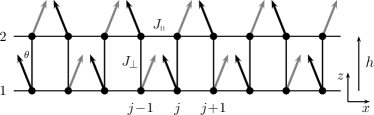
Figure 2: Classical configuration for a spin ladder in the presence of a magnetic field.

In the symmetric action $S_{s}$, we use the duality transformation of the section II, presenting the field $\varphi_{s}$ as a sum of the vortex component $\varphi_{s,v}$ and the vortex-free component $\varphi_{s,t}$. Upon rescaling the time as per $\tau\rightarrow\sqrt{K^{(s)}_{\tau}/K^{(s)}_{x}}\;\tau$, and following the standard steps we obtain

$$S = \int dxd\tau\left\{\phantom{\frac{1}{2}}\frac{1}{2\sqrt{K^{(s)}_{\tau}K^{(s)}_{x}}}\left((\partial_{x}\tilde{\chi})^{2}+(\partial_{\tau}\tilde{\chi})^{2}\right)\right.$$ (28)

$$+ \left.\tilde{\lambda}_{1}\cos{\left(2\pi\left(\tilde{\chi}+2\left(\frac{S-m}{a}\right)x\right)\right)}\phantom{\frac{1}{2}}\!\!\right\}.$$

Now, the cosine term is commensurate if

$$2(S\pm m)\in\mathbb{Z}$$ (29)

Note that, even though our approach does not apply directly to the $m=0$ case, this conditions is nevertheless consistent with the well known $m=0$ plateau for $S=1/2$.

Another important comment is due here. The factor $2$ in front of the Berry term is not an artifact of the transformation (27) because of the periodicity of the fields. Each one of the fields $\phi_{1}$ and $\phi_{2}$ satisfy

$$\phi_{1}(x+L) = \phi_{1}(x)+2\pi n_{1}$$

$$\phi_{2}(x+L) = \phi_{2}(x)+2\pi n_{2}$$

where $n_{1}$ and $n_{1}$ are integers. Then the antisymmetric combination satisfy $\phi_{1}-\phi_{2}=2\pi(n_{1}-n_{2})$. The saddle point solution $\varphi_{a}\equiv 0$ implies $n_{1}=n_{2}$ and then the sum $\phi_{1}+\phi_{2}$ has periodicity $4\pi n_{1}$. The factor $\frac{1}{2}$ in the definition of $\varphi_{s}$ is necessary for the correct periodicity.

III.2 Dimerized spin chain

The dimerized spin chain can be studied in a similar way. We begin with the Hamiltonian

$$H = \sum_{j}\left\{(J+\delta J)\vec{\mathbf{S}}_{1,j}\cdot\vec{\mathbf{S}}_{2,j}+(J-\delta J)\vec{\mathbf{S}}_{2,j}\cdot\vec{\mathbf{S}}_{1,j+1}\right.$$ (30)

$$+ \left.D\left[(\mathbf{S}^{z}_{1,j})^{2}+(\mathbf{S}^{z}_{2,j})^{2}\right]-h\left[\mathbf{S}^{z}_{1,j}+\mathbf{S}^{z}_{2,j}\right]\right\},$$

and use the Eqs. (6), (7) and (II) for each sublattice. We then switch to the path integral formalism, take the continuum limit and drop the constant terms to obtain the following action:

$$S = \int dxd\tau\left\{J\left(\frac{S^{2}-m^{2}}{a}\right)(\phi_{1}-\phi_{2})^{2}\right.$$

$$+ \frac{a}{4}(J-\delta J)(S^{2}-m^{2})\left[(\partial_{x}\phi_{1})^{2}+(\partial_{x}\phi_{2})^{2}\right]$$

$$+ \frac{1}{2}(J-\delta J)(S^{2}-m^{2})(\phi_{1}-\phi_{2})(\partial_{x}\phi_{1}+\partial_{x}\phi_{2})$$

$$+ a\left(J\frac{S^{2}}{S^{2}-m^{2}}+D\right)(\Pi_{1}^{2}+\Pi_{2}^{2})$$

$$+ 2aJ\left(1-\frac{m^{2}}{S^{2}-m^{2}}\right)\Pi_{1}\Pi_{2}$$

$$+ i\left(\frac{S-m}{a}\right)(\partial_{\tau}\phi_{1}+\partial_{\tau}\phi_{2})$$

$$- \left.i(\partial_{\tau}\phi_{1}\Pi_{1}+\partial_{\tau}\phi_{2}\Pi_{2})\right\}.$$

Integrating the $\Pi$-fields and making the substitution $\vec{\varphi}=U\vec{\phi}$ with $U$ given by (27) we have

$$S = \int dxd\tau\left\{4J\left(\frac{S^{2}-m^{2}}{a}\right)\varphi_{a}^{2}\right.$$

$$+ \frac{a}{2}(J-\delta J)(S^{2}-m^{2})\left[(\partial_{x}\varphi_{s})^{2}+(\partial_{x}\varphi_{a})^{2}\right]$$

$$+ 2(J-\delta J)(S^{2}-m^{2})\varphi_{a}\partial_{x}\varphi_{s}$$

$$+ i2\left(\frac{S-m}{a}\right)(\partial_{\tau}\varphi_{s})$$

$$+ \left.\frac{1}{2}\tilde{K}_{\tau}^{(s)}(\partial_{\tau}\varphi_{s})^{2}+\frac{1}{2}\tilde{K}_{\tau}^{(a)}(\partial_{\tau}\varphi_{a})^{2}\right\}.$$

The field $\varphi_{a}$ is massive and we can use the saddle point solution for it $\varphi_{a}=0$. The action for the symmetric field results

$$S_{s} = \int d\tau dx\left\{\frac{1}{2}\tilde{K}_{x}(\partial_{x}\varphi_{s})^{2}+\frac{1}{2}\tilde{K}_{\tau}(\partial_{\tau}\varphi_{s})^{2}\right.$$ (33)

$$+ \left.2i\left(\frac{S-m}{a}\right)(\partial_{\tau}\varphi_{s})\right\}$$

with $\tilde{K}_{x}=a(J-\delta J)(S^{2}-m^{2})$ and $\tilde{K}_{\tau}=1/[a(2J+D)]$.

The action has the same form as for the two-leg ladder and, repeating the steps described in the preceding subsection, we obtain the necessary condition for the formation of magnetization plateaux

$$2(S\pm m)\in\mathbb{Z}.$$ (34)

In both cases studied in this Section, the unit cell contains two spins, and the effective action was written in terms of two fields: $\varphi_{s}$ and $\varphi_{a}$. Notice that, of these two, only the massless one ($\varphi_{s}$) defines the necessary condition for the formation of plateaux.

IV Extensions to $N$-leg ladders and $P$-merized chains.

The arguments, presented in the preceding sections, can be easily extended to more complex models. As we have shown in the previous section, the magnetization processes of a two-leg ladder and of a dimerized chain are described by a single effective action of the massless field, that has the same form for these two different models. Under certain restrictions, this similarity holds for $N$-leg ladders and $N$-merized chains, as well. In the last section we have used two fields to describe the low-energy theory and finally only one field remains massless in our effective action. The extension to the $N$-leg ladder is natural and follows the same steps as in the two legs case but now working with $N$ different fields. The first $N-1$ fields are massive as in the case of $\varphi_{a}$ for the two legs ladder. The effective action can be written also in terms of the last field, which is given by $\varphi_{s}=\frac{1}{N}\sum_{i}\phi_{i}$, and the action is a straightforward generalization of the of equation (28)

$$S = \int dxd\tau\left\{\phantom{\frac{1}{2}}\frac{2\pi^{2}}{\beta^{2}}\left((\partial_{x}\tilde{\chi})^{2}+(\partial_{\tau}\tilde{\chi})^{2}\right)\right.$$ (35)

$$+ \left.\tilde{\lambda}_{1}\cos{\left(2\pi\left(\tilde{\chi}+N\left(\frac{S-m}{a}\right)x\right)\right)}\phantom{\frac{1}{2}}\right\},$$

where $\beta$ depends of the microscopic parameters and the commensurability condition is given by

$$N(S\pm m)\in\mathbb{Z}.$$ (36)

Again, this result contains also what is known for the zero magnetic field. The $N$-leg ladder at zero field was studied by G. Sierra Sierra using the original Haldane’s path integral approach, and the presence of a spin gap was recovered from the condition (36) with $m=0$.

V Adding holes to a single chain

There are several examples of hole-doped magnets. For instance, doping the $S=1$ metal oxide Y₂BaNiO₅metal_oxides with Ca introduces hole carriers in the chains. Other examples are given by manganese oxides such as La_1-xCa_xMnO₃Dagotto_prb_manganites .

Theoretical studies of these compounds generally depart from the double exchange modelDagotto_prl . Using strong Hund’s rule coupling between the itinerant and localized spins, an effective Hamiltonian on a restricted Hilbert space is introduced, where creation of a hole on a given site replaces the spin $S$ on this site by $S-1/2$. Such a calculation of the effective Hamiltonian generalizes the derivation of the $t-J$ model from the Hubbard model for $S=1/2$Zhang_prb . In this section, we study the effect of doping on the low energy physics of a Heisenberg chain and the corresponding effect on the magnetization curve.

We begin with a spin chain with one spin per site in the presence of a magnetic field. Using the path integral formulation, we have shown that the effective action is given by the Eq. (9) of the Section II. Creation of a hole at a given site $j$ corresponds to extracting the spin from this site. To account for this, we will simply remove the contribution that the $j$th spin would have made to the action. Let us introduce at each site a hole creation operator $\psi^{{\dagger}}_{j}$, satisfying fermion commutation relations $\{\psi^{\dagger}_{i},\psi_{j}\}=\delta_{ij}$. Without any holes, we have just the low-energy action (9) of the Section II for the pure spin system.

Important contributions to the action upon creation of a hole are obtained by the change in the interaction between the spins, and simply replacing the Berry term for the spin-$S$ by that for $S-1/2$ for the spin with the hole and then taking into account the contribution to the action due to the hole hopping. We start by considering this very hopping term.

Let $\Omega_{1}$ and $\Omega_{2}$ be the classical spins at sites 1 and 2. According to the arguments of Shankar Shankar , the correct hole hopping term from site 1 to site 2 would not be simply $-t\psi^{{\dagger}}_{2}\psi_{1}$, as such a term would move the hole, but not the spin $\Omega$. At the microscopic level, the electron is transferred by the operator $\mathbf{d}=\sum_{\sigma}\mathbf{c}^{{\dagger}}_{1\sigma}\mathbf{c}_{2\sigma}$, that moves the charge and the spin coherently from 2 to 1. The action of this operator on a state with the hole on site 1 is

$$\mathbf{d}|o,\Omega_{2}\rangle=|\Omega_{2},o\rangle$$ (37)

where $o$ represents a hole. In this language, the correct matrix element for the process is $-t\langle\Omega_{1}|\Omega_{2}\rangle$. Thus, the correct hopping term is $-t\langle\Omega_{1}|\Omega_{2}\rangle\;\psi^{{\dagger}}_{2}\psi_{1}$, where

$$\langle\Omega_{1}|\Omega_{2}\rangle=\left(\cos{\frac{\theta_{1}}{2}}\cos{\frac{\theta_{2}}{2}}+e^{i(\phi_{2}-\phi_{1})}\sin{\frac{\theta_{1}}{2}}\sin{\frac{\theta_{2}}{2}}\right)^{2S}$$ (38)

Notice that, in the $h=0$ case, the classical configuration of the spins is antiparalel and the overlap of coherent states vanishes. Then, in the zero magnetic field case, the hoping amplitude between nearest neighbors is a fluctuating variable with zero average, a very difficult problem to study. This is the main reason for the original problem on hole dopingShankar to concentrate in a model where doping between second neighbors was the dominant effect. In our case, the non zero magnetization implies a non zero overlap between neighboring coherent states allowing for a consistent study of first neighbors hoping problem.

Finally, the hopping of holes is described by the following Hamiltonian

$$H_{hopp}=-t\sum_{j}\langle\Omega_{j}|\Omega_{j+1}\rangle\;\psi^{{\dagger}}_{j+1}\psi_{j}+\mbox{h.c}.$$ (39)

If we expand $\theta$ around the classical energy minimum value $\theta(x)=\theta_{0}+\delta\theta(x)$, we must retain the terms up to order $a$, since the continuum limit $\psi_{j}\rightarrow\sqrt{a}\psi(x)$ for the fermion operators involves an extra factor of $a$. Using the Eq. (6) and retaining terms up to the first order in $a$, we find

$$\langle\Omega_{j}|\Omega_{j+1}\rangle\simeq\left(\frac{m}{S}\right)^{2S}e^{\left(2a\frac{S}{m}\Pi(x)-ia\frac{S}{m}(S-m)\partial_{x}\phi(x)\right)}$$ (40)

then

$$H_{hopp}\!\!\! \!\simeq\!\!\! \!\!-t\sum_{j}\!\left(\frac{m}{S}\right)^{2S}\!\!\!\!\psi^{{\dagger}}_{j+1}\psi_{j}\!\left(\!1\!+\!2a\frac{S}{m}\Pi(x)\!-\!ia\frac{S}{m}(S\!-\!m)\partial_{x}\phi(x)\!\right)$$ (41)

$$+ \mbox{h.c}.$$

Since the sought long-distance physics involves only the states near the Fermi surface, we linearize the theory around $\pm k_{F}$

$$\psi_{j}=e^{ik_{F}aj}\psi_{R,j}+e^{-ik_{F}aj}\psi_{L,j},$$ (42)

to obtain $H_{hopp}=H_{free}+\delta H$, where

$$H_{free} = \sum_{j}-t\cos{k_{F}a}\left[\psi^{{\dagger}}_{R,j+1}\psi_{R,j}+\psi^{{\dagger}}_{R,1}\psi_{R,j+1}\right.$$

$$+ \left.\psi^{{\dagger}}_{L,j+1}\psi_{L,j}+\psi^{{\dagger}}_{L,1}\psi_{L,j+1}\right]$$

$$+ it\sin{k_{F}a}\left[\psi^{{\dagger}}_{R,j+1}\psi_{R,j}-\psi^{{\dagger}}_{R,1}\psi_{R,j+1}\right.$$

$$- \left.\psi^{{\dagger}}_{L,j+1}\psi_{L,j}+\psi^{{\dagger}}_{L,1}\psi_{L,j+1}\right]$$

and

$$\delta H\!\! \!\!=\! \!\!\!-t\left(\frac{m}{S}\right)^{2S}\sum_{j}\left\{4a\frac{S}{m}\cos{(k_{F}a)}\Pi(x)\left(\psi^{{\dagger}}_{R,j}\psi_{R,j}+\psi^{{\dagger}}_{L,j}\psi_{L,j}\right)\right.$$ (44)

$$- \!\!\left.2a\frac{S}{m}(S-m)\sin{(k_{F}a)}\partial_{x}\phi(x)\left(\psi^{{\dagger}}_{R,j}\psi_{R,j}-\psi^{{\dagger}}_{L,j}\psi_{L,j}\right)\right\}$$

Taking the continuum limit $\psi_{j}\rightarrow\sqrt{a}\psi(x)$ and setting the Fermi energy to zero, we obtain

$$H_{hopp}\!\! = \!\!\!\int\!dx\left\{2at\left(\frac{m}{S}\right)^{2S}\!\!\!\sin{(k_{F}a)}\left[\psi^{{\dagger}}_{R}(x)\left(\!-i\partial_{x}\!+\!\frac{S(S-m)}{m}\partial_{x}\phi\right)\psi_{R}(x)-\psi^{{\dagger}}_{L}(x)\left(-i\partial_{x}+\frac{S(S-m)}{m}\partial_{x}\phi\right)\psi_{L}(x)\right]\right.$$ (45)

$$- \left.4atSm^{2S-1}\cos{(k_{F}a)}\Pi(x)\left(\psi^{{\dagger}}_{R}(x)\psi_{R}(x)+\psi^{{\dagger}}_{L}(x)\psi_{L}(x)\right)\right\}$$

Since the linearized theory has an infinite number of particles in the ground state, we shall introduce normal ordering, to correctly define the theory:

$$\psi^{{\dagger}}(x)\psi(x)=\delta+:\psi^{{\dagger}}_{R}(x)\psi_{R}(x)+\psi^{{\dagger}}_{L}(x)\psi_{L}(x):$$ (46)

Now, we account for hole doping. For $S=1/2$, we begin with the action without holes, and remove the Berry phase term at each hole site. For larger values of $S$, we have more than one electron on each site and a hole corresponds to a spin $[S-1/2]$ impurity in the spin-$S$ hostDagotto_prb ; Dagotto_prl ; Sobiella_prl . In other words, we apply the projection operator

$$\mathbf{\mathcal{P}}_{j}=1-\frac{\psi_{j}^{{\dagger}}\psi_{j}}{2S}$$ (47)

to the Berry phase term in the action if the hole was created on site $j$. We must do the same for the spin-spin interaction part using the projector.

$$\mathbf{\mathcal{P}}_{i,j}=(1-\frac{\psi_{i}^{{\dagger}}\psi_{i}}{2S})(1-\frac{\psi_{j}^{{\dagger}}\psi_{j}}{2S}).$$ (48)

Note that this is somehow a different scenario than the one proposed by ShankarShankar where an entire spin $S$ would hope from one site to another. Our approach is more appropriate to cope with the experimental situation we mention below. The modification of our approach to handle Shankar scenario, or any intermediate value of the spin hoping between $S$ and $1/2$ is straightforward.

The following step is to linearize the theory near $\pm k_{F}$, as we did in the hopping term, to obtain

$$\mathbf{\mathcal{P}}_{j} \simeq 1-\frac{\psi_{j}^{{\dagger}}\psi_{j}}{2S}$$

$$= 1-\frac{\delta}{2S}-\frac{1}{2S}:\psi_{R,j}^{{\dagger}}\psi_{R,j}+\psi_{L,j}^{{\dagger}}\psi_{L,j}:$$

where $\delta$ is the noninteracting ground state expectation value. Then, in the presence of doping, the equation (9) reads

$$S_{SM} = \int dxd\tau\left\{\phantom{\frac{1}{2}}\frac{J}{2}\left(1-\frac{\delta}{2S}\right)^{2}a(S^{2}-m^{2})(\partial_{x}\phi)^{2}+a\left(1-\frac{\delta}{2S}\right)^{2}\left(2J+D\right)\Pi^{2}\phantom{\frac{1}{2}}\right\}$$

$$+ i\int dxd\tau\left\{\left(1-\frac{\delta}{2S}\right)\left(\frac{S-m}{a}\right)(\partial_{\tau}\phi)-\left(1-\frac{\delta}{2S}\right)(\partial_{\tau}\phi)\Pi\right.$$

$$- \left.\frac{1}{2S}\left(\frac{S-m}{a}\right)(\partial_{\tau}\phi)(:\psi_{R,j}^{{\dagger}}\psi_{R,j}+\psi_{L,j}^{{\dagger}}\psi_{L,j}:)\right\}.$$

Certain terms have been dropped here as irrelevant in the renormalization group (RG) sense, such as products of normal-ordered fermion operators and bilinears of spin phase operators. As a result, the total action is given by $S_{SM}+S_{hopp}$. Integrating out the $\Pi$ field, we obtain

$$\mathcal{S}_{eff}\!\! = \!\!\int dxd\tau\left\{\phantom{\frac{1}{2}}\frac{1}{2}K_{x}(\partial_{x}\phi)^{2}+\frac{1}{2}K_{t}(\partial_{\tau}\phi)^{2}\right.$$

$$+ \!\!\left.i\left(1-\frac{\delta}{2S}\right)\left(\frac{S-m}{a}\right)(\partial_{\tau}\phi)\right\}$$

$$+ \!\!ig_{1}\!\int\!dxd\tau\left\{\bar{\Psi}(x)\sigma_{3}\left(\partial_{x}\!+\!i\frac{S(S-m)}{m}\partial_{x}\phi\right)\!\Psi(x)\!\right\}$$

$$- \!\!\int dxd\tau\left\{\bar{\Psi}(x)\mathbb{I}\left(\partial_{\tau}-ig_{2}(\partial_{\tau}\phi)\right)\Psi(x)\right\},$$

where

$$\frac{1}{2}K_{x}\!\! = \!\!a\frac{J}{2}\left(1-\frac{\delta}{2S}\right)^{2}(S^{2}-m^{2})$$

$$\frac{1}{2}K_{t}\!\! = \!\!\frac{1}{4a\left(2J+D\right)}$$ (52)

$$g_{1}\!\! = \!\!2at\left(\frac{m}{S}\right)^{2S}\sin{(k_{F}a)}$$

$$g_{2}\!\!\! = \!\!\!\left[\frac{1}{2S}\!\left(\!\frac{S-m}{a}\!\right)\!+\!\frac{2atSm^{2S-1}\cos{(k_{F}a)}}{\left(1\!-\!\frac{\delta}{2S}\right)\left(2J+D\right)}\!\right]$$

$$\Psi(x) = \left(\begin{array}[]{c}\psi_{R}\\ \psi_{L}\end{array}\right)\hskip 22.76228pt\bar{\Psi}(x)=\left(\bar{\psi}_{R},\bar{\psi}_{L}\right).$$ (55)

Upon rescaling time in the fermionic part, we find

$$\mathcal{S}_{eff} = \mathcal{S}_{\phi}+\mathcal{S}_{F}$$ (56)

with

$$\mathcal{S}_{\phi} = \int dxd\tau\left\{\phantom{\frac{1}{2}}\frac{1}{2}K_{x}(\partial_{x}\phi)^{2}+\frac{1}{2}K_{t}(\partial_{\tau}\phi)^{2}\right.$$

$$+ \left.i\left(1-\frac{\delta}{2S}\right)\left(\frac{S-m}{a}\right)(\partial_{\tau}\phi)\right\}$$

$$\mathcal{S}_{F} = i\int dxd\tau\left\{\bar{\Psi}(x)\sigma_{3}\left(\partial_{x}+i\frac{S(S-m)}{m}\partial_{x}\phi\right)\Psi(x)\right\}$$

$$- \int dxd\tau\left\{\bar{\Psi}(x)\mathbb{I}\left(\partial_{\tau}+i\frac{S(S-m)}{m}(\partial_{\tau}\phi)\right)\Psi(x)\right\}$$

$$+ i\int dxd\tau\left\{\bar{\Psi}(x)\mathbb{I}\left(g_{2}+\frac{S(S-m)}{m}(\partial_{\tau}\phi)\right)\Psi(x)\right\}.$$

Now, we write $\phi=\phi_{v}+\phi_{t}$ and then we eliminate the $\phi_{t}$ field from the two first terms of $\mathcal{S}_{F}$ via the change $\Psi\rightarrow e^{-i\frac{S(S-m)}{m}}\Psi$, and by an appropriate rescaling, this effective action can be rewritten in a more compact form:

$$\mathcal{S}_{F}=\int\!dxd\tau\bar{\Psi}\left[-\gamma_{\mu}(\partial_{\mu}+iA_{\mu}+i\tilde{A}_{\mu})\right]\Psi$$ (57)

with

$$A_{\mu}=\frac{S(S-m)}{m}\partial_{\mu}\phi_{v}$$ (58)

and

$$\tilde{A}_{0}=\left(g_{2}+\frac{S(S-m)}{m}\partial_{\mu}\right)\partial_{\tau}(\phi_{v}+\phi_{t})~{};~{}\tilde{A}_{1}=0$$

$$\gamma_{0}=\left(\begin{array}[]{cc}0&-i\\ i&0\end{array}\right)~{};~{}\gamma_{1}=\left(\begin{array}[]{cc}0&1\\ 1&0\end{array}\right).$$ (63)

As we have retained only quadratic terms, we can integrate out the fermionic degrees of freedom. The result is just the determinant of the fermion’s kernel. At this point there is a mathematical observation which is important to stress. The Atiyah-Singer Index theorem stress that the fermionic determinant is non zero only when the gauge fields $A$ and $\tilde{A}$ have zero total magnetic fluxShankar . It can be shown that this condition is automatically satisfied for the field $\tilde{A}$. For the field $A$, the Index theorem then imposes a global constraint that the field $\phi$ have the total vorticity equal to zero, which is nothing else than the charge neutrality of the vortex gas realized by the field $\phi_{v}$.

Once we have integrated out the fermions, we are left with an effective action, which depends only of the scalar field $\phi$. It is basically given by $\mathcal{S}_{\phi}$ in Equation (56) corrected by unimportant gauge invariant counter-terms arising from the fermionic determinant. We then perform the same steps as above, in particular the duality transformation, and get an effective action of the kind:

$$\mathcal{S}_{\phi} = \int dxd\tau\left\{\phantom{\frac{1}{2}}\frac{1}{2K_{\tau}}(\partial_{x}\tilde{\chi})^{2}+\frac{1}{2K_{x}}(\partial_{\tau}\tilde{\chi})^{2}\right.$$

$$+ \left.\lambda_{1}\cos{\left[2\pi\left(\tilde{\chi}+\left(1-\frac{\delta}{2S}\right)\left(\frac{S-m}{a}\right)x\right)\right]}\phantom{\frac{1}{2}}\!\!\!\right\}.$$

In the action above, the cosine term is commensurate when the following condition is satisfied

$$\left(1-\frac{\delta}{2S}\right)\left(\phantom{\frac{1}{2}}\!\!\!\!S-m\right)\in\mathbb{Z}.$$ (65)

Let us now compare the plateau condition (65) for the doped chain to the zero-doping condition (17), namely

$$(S\pm m)\in\mathbb{Z}.$$

The latter emerged from rewriting the Berry phase term in two different yet equivalent ways. Now, if we follow the same arguments and introduce the projectors in the Eqs. (47) and (48), we obtain the two following conditions

$$\left(1-\frac{\delta}{2S}\right)(S\pm m)\in\mathbb{Z}.$$ (66)

Notice that, for $\delta\neq 0$, the two signs in the condition above no longer define the same set of plateau magnetization values comment1 . This inequivalence appeared as a result of passing to the continuum limit and implementing the normal ordering (46). The linear approximation can be implemented provided interference terms due to the Berry phase are properly taken into account, i.e. if there is a value of doping and magnetization, for which vortex configurations are not suppressed by the Berry phase, this should also be true in the linearized theory. Then, in the linearized theory, if one of the conditions in (66) is satisfied, it must manifest itself in the effective action for the scalar field $\phi$ by a commensurate cosine operator. Upon infinitesimal doping, each plateau magnetization value that meets the zero-doping plateau condition

$$(S\pm m)\in\mathbb{Z},$$ (67)

gives rise to two different plateau magnetization values, according to the Eq. (66). However, it is the microscopic details of the model that eventually determine whether the plateau is indeed realized at both of these values, only one of them – or neither.

VI Magnetization plateaux of an anisotropic $S=3/2$ spin chain.

Now, we use the results presented in the preceding sections to study the magnetization plateaux of a simple spin chain. The $S=3/2$ chain with on-site anisotropy has been studied numerically by Okamoto Okamoto and Sakai and Takahashi Sakai . At $D=0$, there are no plateaux in the magnetization curve; as $D$ is increased beyond a critical values $D_{c}$, a plateau appears at $m_{sat}/3$, where $m_{sat}$ denotes the saturation value. With the formalism developped in the sections above, we qualitatively recover these results, and show that the critical value $D_{c}$ decreases upon doping. Indeed, as mentioned above, the stiffness of the field $\tilde{\chi}$ must be such that the cosine operator in (15) be relevant in the renormalization group sense. In the case $\delta=0$, our computation shows that this is achieved for values of $D$ greater than $D_{c}=0.467$, a value to be compared with the result of Okamoto and Kitazawa ($D_{c1}=0.387$) .

In the presence of doping, the Hamiltonian contains lattice $S=3/2$ spins and spin-1 mobile “holes”, and can be obtained from a Kondo lattice model Dagotto_prb . It has the form

$${\cal H}=\sum_{\langle ij\rangle}-t\hat{T}+J\vec{S}_{i}\cdot\vec{S}_{j}+\sum_{i}D(S_{i}^{z})^{2},$$ (68)

where the kinetic energy term acts as per

$$\hat{T}|3/2,m\rangle|1,m^{\prime}\rangle = A|1,m+1/2\rangle|3/2,m^{\prime}-1/2\rangle$$ (69)

$$+ B|1,m-1/2\rangle|3/2,m^{\prime}+1/2\rangle$$

with $A=\sqrt{(2-m^{\prime})(3/2-m)}/3$ and $B=\sqrt{(2+m^{\prime})(3/2+m)}/3$. In other words, the local magnetization can only change by 1/2 since it comes originally from the hopping of spin-1/2 electrons.

Upon doping, we expect the plateau to split into two. The necessary condition for the formation of magnetic plateaux in the spin-$3/2$ chain is given by

$$(1-\frac{\delta}{3})(\frac{3}{2}-m)\in\mathbb{Z}$$ (70)

For a small enough $\delta$ we obtain the following possible plateaux

$$\tilde{m}_{\pm}=\frac{1}{3}(1\pm\delta)\;\;\hbox{and}\;\;\tilde{m}_{s}=1-\frac{\delta}{3}$$ (71)

where $\tilde{m}=(1-\frac{\delta}{2S})\frac{m}{S}$.

In order to check these predictions, we have performed numerical simulations using the powerful DMRG algorithm dmrg for various dopings at a fixed large $D/J=5$, and with open boundary conditions (OBC) for system lengths up to $64$. Typically, we kept up to 1200 states, which is sufficient to have a discarded weight smaller than $10^{-12}$.

The DMRG results are showed in Fig. 3. Without doping, the large on-site anisotropy $D$ stabilizes a wide magnetization plateau at $M_{s}/3$ in agreement with previous studies Okamoto ; Sakai . Now, doping with $S=1$ impurities splits this plateau, in perfect agreement with our prediction.

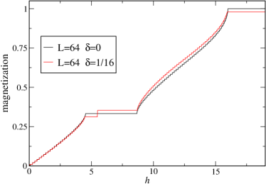
Figure 3: (Color online) Magnetization curve ($\tilde{m}$) for the $S=3/2$ chain corresponding to $D/J=5$ obtained with DMRG.

VII Holes in $N$-leg ladders and $p$-merized chains

In more complex models such as $N$-leg ladders and $p$-merized chains, the contribution of doping can be traced similarly to how it was done in the Section V. Here, we briefly discuss the approach for the case of ladders. The $p$-merized chain follows the same steps. First we note that the hopping constant must be replaced by $t_{\alpha,\beta}=-t\langle\Omega_{\alpha,j}|\Omega_{\beta,j+1}\rangle$, where the indices $\alpha$ and $\beta$ label the chains of the ladder. We need to define $N$ kinds of holes corresponding to each chain. Then we have two kinds of hopping terms, the hopping in each chain ($t_{\alpha,\alpha}$) and the interchain hopping ($t_{\alpha,\beta}$, with $\alpha\neq\beta$). Straightforward calculations give

$$\!\!t_{\alpha,\alpha} \simeq t\left(\frac{m}{S}\right)^{2S}\!\!\exp{\left[2a\frac{S}{m}\Pi_{\alpha}-ia\frac{S}{m}(S-m)\partial_{x}\phi_{\alpha}\right]}$$ (72)

$$\!\!t_{\alpha,\beta} \simeq t\left(\frac{m}{S}\right)^{2S}\!\!\exp{\left[2a\frac{S}{m}(1-i(\frac{\phi_{\alpha}-\phi_{\beta}}{2}))(\Pi_{\alpha}-\Pi_{\beta})\right]}$$ (73)

$$\times \exp{\left[i2\frac{S}{m}(S-m)(\frac{\phi_{\alpha}-\phi_{\beta}}{2})\right]}.$$

Now, we can write the kinetic Hamiltonian for the fermions and linearize the spectrum as before. In the spin part and the Berry phase contribution we must insert the corresponding projectors $1-\frac{\psi^{{\dagger}}_{\alpha}\psi_{\alpha}}{2S}$ and $(1-\frac{\psi^{{\dagger}}_{\alpha}\psi_{\alpha}}{2S})(1-\frac{\psi^{{\dagger}}_{\beta}\psi_{\beta}}{2S})$. The procedure is a straightforward extension of the spin chain case: we must integrate over the $\Pi_{\alpha}$ fields and use the Hubbard-Stratonovich auxiliary fields as in the case of the spin chain, decoupling each field $\phi_{\alpha}$ as $\phi_{\alpha}=\phi_{\alpha,v}+\phi_{\alpha,t}$. The first $N-1$ fields are massive and can be evaluated in the saddle point solution. Once we have integrated out the fermions, we finally obtain the following result for the effective action

$$S_{eff}^{ladder}\!\!\! = \!\!\!\int dxd\tau\left\{\!\!\!\!\phantom{\frac{1}{2}}\frac{1}{2K_{\tau}}(\partial_{x}\tilde{\chi})^{2}+\frac{1}{2K_{x}}(\partial_{\tau}\tilde{\chi})^{2}\right.$$

$$+ \!\!\!\left.\lambda_{1}\cos{\left(2\pi\left(\tilde{\chi}+N\left(1\!-\!\frac{\delta}{2S}\right)\left(\frac{S\!-\!m}{a}\right)x\right)\right)}\phantom{\frac{1}{2}}\!\!\!\right\}.$$

The final condition for the formation of magnetization plateaux reads

$$N\left(1-\frac{\delta}{2S}\right)\left(S\pm m\right)\in\mathbb{Z}.$$ (75)

The calculation for the $N$-merized chain is straightforward and gives the condition (75).

For the case of the two-leg ladder, plateaux at irrational values controlled by doping have been predicted by bosonization Cabra_irrational and numerically supported by numerical results Roux_irrational ; Roux_2007 . In our approach the condition for the formation of magnetization plateaux in a $S=1/2$ two legs ladder with doping reads

$$2(1-\delta)(S-m)\in\mathbb{Z}$$ (76)

where the magnetization per site takes values between $-S\leq m\leq S$. To compare with the results in Refs.Cabra_irrational, and Roux_irrational, ; Roux_2007, we must properly normalize the magnetization as $\tilde{m}=\frac{(1-\delta)}{S}m$, and then, for $S=1/2$ the condition reads

$$1-\delta\pm\tilde{m}\in\mathbb{Z}$$ (77)

which is identical to the condition used in Ref. Roux_irrational, based on the OYA criterion OYA . For small $\delta$ we expect possible plateaux at $\tilde{m}=1-\delta$ and $\tilde{m}=\delta$, which has been confirmed numerically with DMRG (See Fig. 3 of Ref. Roux_2007, ).

VIII Trimerized chain

In this section we study a $S=1/2$ trimerized chain in a magnetic field. Although the main goal of this section is to test our procedure developped in the previous sections against the numerical results, obtained by means of DMRG simulations, the study of this model in the presence of doping is interesting by itselfCabra_phys_lett_a . For instance, the antiferromagnetic $S=1/2$ trimerized chain has experimental realizations such as the synthesized copper hydroxydiphosphate Cu₃(P₂O₆OH)₂, where a $1/3$ magnetization plateau has been observed Hase_2006 .

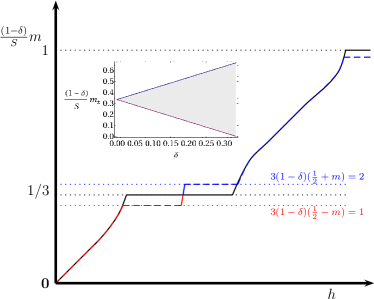
Figure 4: (Color online) Schematic magnetization curve for the $S=1/2$ trimerized chain. The solid line corresponds to $\delta=0$ and the dashed red(blue) one to $\delta\neq 0$. In the inset we show the position of the possible magnetization plateaux as a function of $\delta$.

The Hamiltonian of the $S=1/2$ trimerized chain can be written as

$$H = J\sum_{j}(\vec{\mathbf{S}}_{j,1}\cdot\vec{\mathbf{S}}_{j,2}+\vec{\mathbf{S}}_{j,2}\cdot\vec{\mathbf{S}}_{j,3})$$

$$+ \frac{\gamma J}{2}\sum_{j}(\vec{\mathbf{S}}_{j-1,3}\cdot\vec{\mathbf{S}}_{j,1}+\vec{\mathbf{S}}_{j,3}\cdot\vec{\mathbf{S}}_{j+1,1})$$

$$- h\sum_{j}\sum_{\alpha=1}^{3}\mathbf{S}^{z}_{j,\alpha}$$

where $J$ is the intra-trimer coupling and $\gamma J$ the inter-trimer one. The first subscript $j$ labels a trimer, while the second subscript labels the spins within the trimer. We proceed as in the case of the dimerized chain – except that now we work with three fields corresponding to the three different spins in each trimer. Eventually, only one field remains massless in the effective action, which is a straightforward generalization of the Eq. (10). The commensurability conditions are given by the Eq. (75) with $N=3$ and $S=1/2$:

$$3(1-\delta)(\frac{1}{2}\pm m)\in\mathbb{Z}$$ (79)

where we take $-\frac{1}{2}\leq m\leq\frac{1}{2}$. For $\delta=0$ a magnetization plateau is expected at $m/m_{sat}=1/3$. In the presence of doping, the plateau is expected to split into two different plateaux, located at

$$\frac{m_{\pm}}{S}=\frac{1}{3}\left(\frac{1\pm 3\delta}{1-\delta}\right)$$ (80)

As usual, a simple way to introduce doping is to consider a $t-J$ hamiltonian:

$$H = \sum_{\langle ij\rangle}J_{ij}(\vec{\mathbf{S}}_{i}\cdot\vec{\mathbf{S}}_{j}-\frac{1}{4}n_{i}n_{j})-\sum_{\langle ij\rangle,\sigma}t_{ij}(c^{\dagger}_{i\sigma}c_{i\sigma}+h.c)$$ (81)

$$- h\sum_{j}\sum_{\alpha=1}^{3}\mathbf{S}^{z}_{j,\alpha}$$

where the double occupancy is forbidden on each site, the magnetic exchange and hopping amplitudes are equal, respectively, to $J$ and $t$ for intra-trimer bonds – and to $\gamma J$ and $\sqrt{\gamma}\,t$ for inter-trimer bonds. Note that we have used an inter-trimer hopping amplitude of $t^{\prime}=\sqrt{\gamma}t$ in order to be consistent with the magnetic exchange anisotropy $(t^{\prime}/t)^{2}=\gamma$.

In the Fig. 4, we show a schematic magnetization curve for the $S=1/2$ trimerized chain with the above parameters. We plot the normalized magnetization $\tilde{m}=\frac{(1-\delta)}{S}m$ in order to compare with the numerical results obtained by DMRG. In terms of $\tilde{m}$, the two plateaux are predicted to satisfy

$$\tilde{m}_{\pm}=\frac{1}{3}\pm\delta$$ (82)

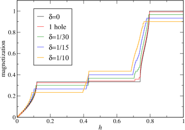
Figure 5: (Color online) Magnetization $\tilde{m}$ for the $S=1/2$ trimerized chain with $\gamma=1/4$ and $J/t=0.5$, obtained by DMRG simulations for different values of the filling on chain of length $L=120$. A splitting (proportional to doping) in the magnetization plateau is clearly observed for non-zero doping.

The DMRG results are shown in the Fig. 5 for a chain of length $L=120$ with OBC. Parameters of the $t-J$ model are $J/t=0.5$ and an anisotropy $\gamma=1/4$. Typically, we keep up to 1200 states, which is sufficient to have a discarded weight smaller than $10^{-9}$. In the absence of doping, our choice of strong anisotropy leads to a wide plateau at $m_{sat}/3$. For a finite doping of the order of $10\%$, our numerical data are in perfect agreement with our prediction: the plateau is split and the splitting is simply proportional to doping. Between the plateaux, the magnetization curve is smooth (the steps are only finite-size effects). However, for very small doping, we observe a strange shape of the magnetization curve just above the upper split plateau. This phenomenon can already be observed for a chain doped with a single hole, and it is likely to stem from the existence of a bound state between a hole and a polarized trimer (“magnon”). The same mechanism is at work for instance in lightly doped two-leg ladders Troyer1996 ; Poilblanc2004 , where a hole pair-magnon bound state emerges, leading to an irrational magnetization plateau Roux_irrational . The formation of such bound states is generic in $t-J$ models due to the Nagaoka effect Nagaoka : holes gain kinetic energy in a ferromagnetic environment. We have not investigated in detail how this bound-state will modify the magnetization curve in our case, but our data clearly show that the magnetization curve has two different regimes in the upper part.

IX Summary and conclusions

Systems with strong easy-axis anisotropy are likely to show plateaux in the magnetization curve even at the classical level. One peculiarity of such plateaux is that the spin configuration must be collinear, i.e. all the spins of the system must be pointing in the same direction LhuiMis . In the present work, we have studied the plateaux that are intrinsically quantum-mechanical: the magnetization curve of the corresponding classical system would remain a straight line all the way to the saturation point. This observation urges one to look for a theory, that would clearly identify the quantum-mechanical effects behind the plateaux. And this was precisely the achievement of Tanaka, Totsuka and Hu Tanaka . A key advantage of their approach versus the abelian bosonization is the applicability of the former in more than one spatial dimension.

We have seen that, within the path integral approach, all the information relevant for the presence of a plateau is encapsulated in the Berry phase term. The topological nature of the Berry phase and its expression in terms of quantized vorticity play a crucial role here. Moreover, even though the path integral approach is based on the coherent-state description, developped for higher spins $S\gg 1$, the topological (quantized) nature of the Berry phase serves as a protection that makes it exact even for spin-$1/2$. To be more precise – given a value of the plateau magnetization, the critical values of the microscopic parameters for the opening of the plateau are sensitive to the choice of a cut-off procedure, and subject to $1/S$ corrections, which renders their accurate calculation difficult. However, the values of the plateau magnetization itself, defined by the necessary condition above, are exact.

In this paper, we have extended the TTH approach to the presence of doping, and have shown that the doping-dependent splitting of the magnetization plateaux is a generic feature that goes beyond spin $1/2$ Hubbard or $t-J$ models. We have tested the validity of the approach by verifying some of the well-known results for undoped and doped spin-$1/2$ chains and ladders plateaux_ladd ; Plateaux_pmer ; Cabra_irrational ; Poilblanc2004 ; Roux_irrational ; Roux_2007 ; Roux_PhD . Then, to illustrate the power of the approach, we have studied a doped higher-spin system that would present a problem for a rigorous treatment via traditional bosonization technique. In contrast to the zero-magnetization case, initially treated by Shankar, here we have successfully used the path integral approach in the case of doped systems with nearest-neighbor hopping only. To the best of our knowledge, this work also offers the first description of a doped antiferromagnetic system in the presence of a magnetic field within the path integral approach. Our analytical calculations have been supplemented by DMRG numerical work in two key examples of doped systems, the trimerized spin $1/2$ chain, and a spin $3/2$ chain. All of our results are represented by the Eq. (2), but in fact this approach is applicable far beyond the examples given in the paper. It appears that now we have a reasonably controlled technique to study the origin of magnetization plateaux in system with arbitrary spin, dimensionality and doping. This is to be contrasted to other techniques that are limited either to one dimension (such as bosonization or DMRG), or to spin-$1/2$ (such as numerical diagonalization in dimensions $D\geq 2$, or bond-operator/hard core bosons descriptions).

- (1) F.M.D. Haldane, Phys. Rev. Lett. 50, 1153 (1983)
- (2) M. Oshikawa, M. Yamanaka, and I. Affleck. Phys. Rev. Lett. 78, 1984 (1997) M. Oshikawa and I. Affleck, Phys. Rev. Lett. 79, 2883 (1997)
- (3) D.C. Cabra, A. Honecker, and P. Pujol, Phys. Rev. Lett. 79, 5126 (1997); D.C. Cabra, A. Honecker, and P. Pujol, Phys. Rev. B 58, 6241 (1998);
- (4) K. Totsuka, Phys. Lett. A 228 103 (1997); Phys. Rev. B 57, 3454 (1998) D. C. Cabra and M. D. Grynberg Phys. Rev. B 59, 119 (1999) ; K. Hida and I. Affleck, J. Phys. Soc. Jpn. 74, 74 (2005); D.C. Cabra, C.J. Gazza, C.A. Lamas and H.D. Rosales, Phys. Rev. B 83, 224406 (2011).
- (5) S. Miyashita, J. Phys. Soc. Jpn. 55, 3605 (1986); A. Chubukov and D. I. Golosov, J. Phys. Condens. Matter 3, 69 (1989).
- (6) D.C. Cabra, A. De Martino, M. D. Grynberg, S. Peysson and P. Pujol, Phys. Rev. Lett. 85, 4791 (2000); P. Pujol and J. Rech, Phys. Rev. B 66, 104401 (2002); C.A. Lamas, D.C. Cabra, M.D. Grynberg, and G.L. Rossini, Phys. Rev. B 74, 224435 (2006).
- (7) D. C. Cabra, A. De Martino, P. Pujol, and P. Simon, Europhys. Lett. 57 402 (2002); D.C. Cabra, A. De Martino, A. Honecker, P. Pujol, and P. Simon, Phys. Rev. B 63, 094406 (2001)
- (8) D. Poilblanc, E. Orignac, S. R. White, and S. Capponi, Phys. Rev. B 69, 220406(R) (2004).
- (9) G. Roux, S.R. White, S. Capponi, and D. Poilblanc, Phys. Rev. Lett. 97, 087207 (2006)
- (10) Y. Nagaoka, Phys. Rev. 147, 392 (1966).
- (11) G. Roux, E. Orignac, P. Pujol, and D. Poilblanc, Phys. Rev. B 75, 245119 (2007)
- (12) For three-leg t-J ladders, doping can split the 1/3 plateau, see G. Roux, Ph.D. thesis, Toulouse University (2007), available at http://tel.archives-ouvertes.fr/tel-00167129/fr.
- (13) T. Momoi and K. Totsuka, Phys. Rev. B 61, 3231 (2000)
- (14) A. Tanaka, K. Totsuka, and X. Hu, Phys. Rev. B 79, 064412 (2009)
- (15) S. Michimura, et al., Physica B 378-380, 596 (2006); S. Yoshii, et. al., J. Magn. and Magn. Mat. 310, 1282 (2007); F. Iga, et al., J. Magn. and Magn. Mat. 310, e443 (2007).
- (16) R. Shankar. Phys. Rev. Lett. 63, 203 (1989); Nucl. Phys B330, 433 (1990).
- (17) E.H. Lieb, T.D. Schultz, and D.C. Mattis, Ann. Phys. (N.Y.) 16, 407 (1961)
- (18) C. K. Majumdar and D. K. Ghosh, J. Math. Phys. 10, 1392 (1969), J. Math. Phys. 10, 1399 (1969); F. D. M. Haldane, Phys. Rev. B 25, 4925 (1982), Phys. Rev. B 26, 5257 (1982).
- (19) B. C. Watson, V. N. Kotov, and M.W. Meisel, Phys. Rev. Lett. 86, 5168 (2001)
- (20) G. Sierra, J. Phys. A 29, 3299 (1996)
- (21) A. P. Ramirez, S-W. Cheong, and M. L. Kaplan, Phys. Rev. Lett. 72, 3108 (1994).
- (22) E. Dagotto et. al., Phys. Rev. B 58, 6414 (1998)
- (23) E. Dagotto, J. Riera, A. Sandvik, and A. Moreo , Phys. Rev. Lett. 76, 1731 (1996)
- (24) F. C. Zhang and T. M. Rice , Phys. Rev. B 37, 3759 (1988)
- (25) E. Müller-Hartmann and E. Dagotto, Phys. Rev. B 54, R6819 (1996)
- (26) H. Frahm and C. Sobiella, Phys. Rev. Lett. 83, 5579 (1999)
- (27) In fact, it can be shown that these two conditions are equivalent only in the case of a vortex-free configuration of the field.
- (28) K. Okamoto and A. Kitazawa, Journal of Physics and Chemistry of Solids 62, 365 (2001)
- (29) T. Sakai and M. Takahashi, Phys. Rev. B 57, R3201 (1998)
- (30) S. R. White, Phys. Rev. Lett. 69, 2863 (1992).
- (31) D. C. Cabra, A. De Martino, A. Honecker, P. Pujol and P. Simon, Phys. Lett. A, 268, 418 (2000)
- (32) M. Hase et. al., Phys. Rev. B 73, 104419 (2006)
- (33) M. Troyer, H. Tsunetsugu, and T.M. Rice, Phys. Rev. B 53, 251 (1996).
- (34) C. Lhuillier and G. Misguich, Frustrated Quantum Magnets in HIGH MAGNETIC FIELDS, Lecture Notes in Physics, 2002, Volume 595, (2002).