Casimir interaction between topological insulators with finite surface band gap

Abstract

Casimir interaction between topological insulators with opposite topological magnetoelectric polarizabilities and finite surface band gaps has been investigated. For large surface band gap limit$(m\rightarrow\infty)$, we can obtain results given in [Phys. Rev. Lett. 106, 020403 (2011)]. For small surface band gap limit$(m\rightarrow 0)$, Casimir interaction between topological insulators is attractive and analogy to ideal mental in short separation limit. Generally, there is a critical value $m_{c}$ and when the surface band gap is greater than the critical value, the Casimir force is repulsive in an intermediate separation region. We estimate the critical surface band gap $m_{c}\sim 1/(2a)$, where $a$ is a critical separation where Casimir force vanishes.

I Introduction

Time reversal invariant topological insulator(TI)Qi_physToday_2010 (1, 2, 3) is a new quantum state of matter which has a full insulating gap in the bulk, but has gapless surface states protected topologically. This material has been extensively studied experimentallyHsieh_nature_2008 (4, 5, 6, 7, 8, 9) and theoreticallyFu_prl_2007 (10, 11, 12, 13). Two dimensional TI has been observed in HgTe quantum wellBernevig_science_2006 (14, 15), $\text{Sb}_{1-x}\text{Te}_{x}$ is the first material has been reported to be 3-dimensional TI, and $\text{Bi}_{2}\text{Se}_{3}$, $\text{Bi}_{2}\text{Te}_{3}$, $\text{Sb}_{2}\text{Te}_{3}$ have been predictedHJZhang_nature_2009 (16) to be TI with single Dirac cone on the surface. Novel properties of TI have been predicted, for instance, effective monopoleQi_science_2009 (17) and topological magnetoelectric effectQi_prb_2008 (13), superconductor proximity effect induced Majorana fermion statesFu_prl_2008 (18) etc.

Recently, an interesting property of TI, tunable repulsive Casimir interaction between TIs with opposite topological magnetoelectric polarizability $\theta$ has been proposedGrushin_PRL (19), and the robustness of this repulsion in small separation limit against finite temperature and uniaxial anisotropy has also been analyzedGrushin_arXiv (20). Repulsive Casimir interaction has been discussed in a few proposals, with special geometryLevin_prl_2010 (21) or chiral metamaterialsZhao_prl_2009 (22), or filling high-refractive liquid between dielectricsZwol_pra_2010 (23). The repulsion between TIs is analogy to metamaterials, however, time reversal invariant TI is protected by gapless surface states. In order to observe the repulsive Casimir interaction, one need cover the TI surfaces with magnetic coating to open the band gap. The effect of finite surface band gap on this repulsive force is considerable.

In this paper, we analyze the influence of finite surface band gap on Casimir force between TIs with opposite topological magnetoelectric polarizability $\theta$, we show that there is a minimal surface band gap $m_{c}$ and when surface band gap $m<m_{c}$, repulsive Casimir force will disappear. We also estimate this critical surface band gap numerically.

Let us formulate the model. When time reversal symmetry is protected in the bulk, the topological nontrivial term $\alpha/(4\pi^{2})\int{d^{3}}{x}{d}t\theta\bm{E}\cdot\bm{B}$ can be reexpressed as spin-momentum locked fermions on the interface of TI and normal insulator, in this paper we consider only one kind of fermion corresponding to $\theta=\pi$ or $-\pi$, generalization to multi-fermions is straightforward. Action of Dirac fermion on TI surface is

$$S_{D}={\int}d^{3}x\,\bar{\psi}\left[i\gamma^{a}(\partial_{a}+ieA_{a})-m\right]\psi,$$ (1)

where $a=0,x,y$, $\gamma^{0}=\sigma^{z}$, $\gamma^{x}=iv_{F}\sigma^{y}$, $\gamma^{y}=-iv_{F}\sigma^{x}$. $\sigma^{x,y,z}$ are Pauli matrices of spin, $v_{F}$ is the Fermi velocity of surface fermion, which has a magnitude of $10^{-3}$ speed of light(we set $\hbar=c=1$ in this paper) and takes different values for different materialsYLChen_science_2009 (5, 6), ie, $v_{F}=1.3\times 10^{-3}$ for $\text{Bi}_{2}\text{Te}_{3}$, and $1.7\times 10^{-3}$ for $\text{Bi}_{2}\text{Se}_{3}$. Parameter $m$ is surface band gap opened by magnetic coating on TI and we assume chemical potential has been tuned into the surface band gap. $A_{a}$ present the first three components of vector-potential, while electromagnetic field is described by Maxwell action:

$$S_{EM}=-\frac{1}{8\pi}{\int}d^{4}x(\varepsilon\bm{E}^{2}-\frac{1}{\mu}\bm{B}^{2}),$$ (2)

where $\bm{E}$ and $\bm{B}$ are electric and magnetic fields, $\varepsilon$ and $\mu$ are permittivity and permeability of TI in the bulk and equal to 1 in the vacuum.

This paper is organized as follows: In Sec. II, we evaluate an effective action for electromagnetic field on TI surface by quantum field theory approach and give the Maxwell equations of electromagnetic field with proper boundary conditions. In Sec. III, we analyze the Casimir interaction between TIs via Lifshitz theory. We discuss the results in Sec. IV, and give a conclusion in Sec. V.

II Effective Lagrangian on TI Surface and Maxwell Equations

In order to calculate the Casimir interaction caused by quantum fluctuation of electromagnetic field between TIs, one need to integrate the contribution from surface fermion. An effective action for external electromagnetic field in (2+1)-dimension can be found by standard quantum field theory approachchay1993 (24, 25, 26), $S_{eff}(A)=-i\ln\det[i\gamma^{a}(\partial_{a}+ieA_{a})-m]$. We introduce a Feynman parameter, integrate out the fermion field up to one-loop correction and get the effective action in the following form:

$$S_{eff}(A) = \int{d}^{3}{x}\left[-\frac{\phi(\lambda)}{8\pi}\epsilon_{abc}A^{a}\partial^{b}A^{c}\right.$$ (3)

$$+ \left.\frac{\Phi(\lambda)}{4{\pi}|m|}\left(F_{0j}F^{0j}+v_{F}^{2}F_{xy}F^{xy}\right)\right],$$

with dimensionless parameters $\phi$ and $\Phi$ which take the forms:

$$\phi(\lambda) = \text{sign}(m)\alpha\int_{0}^{1}{dx}\frac{1}{\sqrt{1-x(1-x)\lambda}},$$ (4)

$$\Phi(\lambda) = \alpha\int_{0}^{1}{dx}\frac{(1-x)x}{\sqrt{1-x(1-x)\lambda}},$$ (5)

where $\text{sign}(m)$ gives the sign of surface band gap, which corresponding to different signs of topological magnetoelectric polarizability. $\alpha=1/137$ is the fine structure constant of electromagnetic interaction, $\lambda=\left[k_{0}^{2}-v_{F}^{2}\left(k_{x}^{2}+k_{y}^{2}\right)\right]/{m^{2}}$, and $k_{0}$, $k_{x}$, $k_{y}$ are frequency and momentum of electromagnetic fields on TI surface. A detailed derivation and a short discussion on this effective action(3) have been given in the appendix. We also note that in both limit, $m^{2}\rightarrow 0$ and $m^{2}\rightarrow\infty$, $\phi$ and $\Phi$ are convergent. For the sake of Eq.(20), we derive expressions of $\phi$ and $\Phi$ in imaginary time formalism:

$$\tilde{\phi}(\gamma) = \text{sign}(m)\frac{2\alpha}{\sqrt{\gamma}}\arctan\left(\frac{\sqrt{\gamma}}{2}\right),$$ (6)

$$\tilde{\Phi}(\gamma) = \frac{\alpha}{2\gamma}+\left(\frac{\alpha}{4\sqrt{\gamma}}-\frac{\alpha}{\gamma^{3/2}}\right)\arctan\left(\frac{\sqrt{\gamma}}{2}\right),$$ (7)

where $\gamma=(k_{0}^{2}+v_{F}^{2}\left(k_{x}^{2}+k_{y}^{2}\right))/{m^{2}}$. For the large surface band gap limit $(|m|\rightarrow\infty)$, $\tilde{\phi}(\gamma)\rightarrow{\text{sign}(m)}\alpha$, the term proportional to $\phi(\lambda)$ in Eq.(3) is topological and the term proportional to $\Phi(\lambda)$ in Eq.(3) is vanishing. For the small gap limit $(|m|\rightarrow 0)$, $\tilde{\phi}(\gamma)\rightarrow 0$ and $\tilde{\Phi}(\gamma)\rightarrow 1/6$.

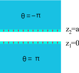
Figure 1: Schematic illustration of Casimir interaction between TIs with opposite topological magnetoelectric polarizability $\theta$. We assume the thickness of magnetic coating is much smaller than the separation between TIs.

Add the surface term Eq.(3) to standard action of electromagnetic fields Eq.(2), one can get the Maxwell equations with surface corrections:

$$\frac{1}{4\pi}\nabla\cdot\bm{D}=-\delta(z-z_{i})\left(\frac{\phi_{i}}{4\pi}B_{z}-\frac{\Phi}{2\pi|m|}\nabla\cdot\bm{E}\right),$$ (8)

$$\frac{1}{4\pi}\left[\partial_{t}\bm{D}-(\nabla\times\bm{H})\right]$$

$$=\delta(z-z_{i})\left[\frac{\phi_{i}}{4\pi}\tilde{\bm{E}}+\frac{\Phi}{2\pi|m|}\left(\partial_{t}\bm{E}-v_{F}^{2}\nabla\times\bm{B}\right)\right],$$ (9)

$$\nabla\cdot\bm{B}=0,$$ (10)

$$\partial_{t}\bm{B}+(\nabla\times\bm{E})=0,$$ (11)

where $\bm{D}=\varepsilon\bm{E}$ and $\bm{H}=\bm{B}/\mu$ are electric displacement field and magnetizing field, $\tilde{E}_{j}=\epsilon_{jk}E_{k}$ ($j,k=x,y$), ($i=1,2$), $z_{1}=0$ and $z_{2}=a$ are positions of TI-surfaces (as shown in Fig.[1]), $\phi_{1}$ and $\phi_{2}$ are corresponding values of $\phi$. Without loss of generality, we assume the absolute values of surface band gaps on two TIs are equal, different signs of surface band gaps stand for different signs of the topological term $\alpha\theta\bm{E}\cdot\bm{B}/(4\pi^{2})$ in Lagrangian of electromagnetic fields in TIs. We also note that in large band gap limit $(|m|\rightarrow\infty)$, these Maxwell equations are equal to those given in Refs.Qi_science_2009 (17, 27) by redefine the electric displacement and magnetizing field as $\bm{D}=\varepsilon\bm{E}+{\alpha}\frac{\theta}{\pi}\bm{B}$, $\bm{H}=\frac{1}{\mu}\bm{B}-{\alpha}\frac{\theta}{\pi}\bm{E}$. From above Maxwell equations, we get the following discontinuous boundary conditions:

$$D_{z}(z_{i}^{+})-D_{z}(z_{i}^{-}) = -{\phi_{i}}B_{z}+\frac{2\Phi}{|m|}\left(\partial_{x}E_{x}+\partial_{y}E_{y}\right)$$ (12)

$$H_{x}(z_{i}^{+})-H_{x}(z_{i}^{-}) = {\phi_{i}}E_{x}-\frac{2\Phi}{|m|}\left(\partial_{t}E_{y}+v_{F}^{2}\partial_{x}B_{z}\right)$$ (13)

$$H_{y}(z_{i}^{+})-H_{y}(z_{i}^{-}) = {\phi_{i}}E_{y}+\frac{2\Phi}{|m|}\left(\partial_{t}E_{x}-v_{F}^{2}\partial_{y}B_{z}\right),$$ (14)

where $z_{i}^{\pm}$ means $z_{i}\pm 0$. And $E_{x}$, $E_{y}$, $B_{z}$ are continuous on the interfaces.

III Casimir Interaction

Now we analyze the Fresnel coefficients of reflection light on the TI-vacuum interface. Incident TE-mode from vacuum with wave-vector $(k_{x},k_{y},k_{z})$ will induce reflected TE and TM-mode, we assume the reflection coefficients are $r_{ee}$ and $r_{em}$ respectively, then the electromagnetic waves in the vacuum read:

$$\bm{E} = (1+r_{ee})k_{0}(-k_{y}\bm{e}_{x}+k_{x}\bm{e}_{y})+r_{em}(-k_{z}\bm{k}-k^{2}\bm{e}_{z}),$$

$$\bm{B} = (-k_{z}\bm{k}+k^{2}\bm{e}_{z})+r_{ee}(k_{z}\bm{k}+k^{2}\bm{e}_{z})$$ (15)

$$+r_{em}k_{0}(-k_{y}\bm{e}_{x}+k_{x}\bm{e}_{y}),$$

and the refracted light with TE, TM-mode in TI take the forms:

$$\bm{E} = t_{ee}k_{0}(-k_{y}\bm{e}_{x}+k_{x}\bm{e}_{y})+c\,t_{em}(p_{z}\bm{k}-k^{2}\bm{e}_{z}),$$

$$\bm{B} = t_{ee}(-p_{z}\bm{k}+k^{2}\bm{e}_{z})+\frac{t_{em}}{c}k_{0}(-k_{y}\bm{e}_{x}+k_{x}\bm{e}_{y}),$$ (16)

where $t_{ee}$ and $t_{em}$ are refraction coefficients of TE and TM-mode, $c$ is the relative velocity of light in TI bulk, $\bm{k}=k_{x}\bm{e}_{x}+k_{y}\bm{e}_{y}$, $k^{2}=k_{x}^{2}+k_{y}^{2}$ and $p_{z}$ is $z$-component of wave vector in TI. For the injected TM-mode, one can write the analogy equations with reflection coefficients $r_{me}$, $r_{mm}$ and refraction coefficients $t_{me}$, $t_{mm}$. After some tedious derivation, we obtain the Fresnel coefficients matrix $\mathcal{R}$ in imaginary time formalism:

$$\mathcal{R}=\left(\begin{array}[]{cc}r_{ee}&r_{em}\\ r_{me}&r_{mm}\\ \end{array}\right),$$ (17)

with

$$r_{ee} = -1+\frac{2}{D}\left(1+\varepsilon\frac{k_{z}}{p_{z}}+2\tilde{\Phi}\frac{k_{z}}{m}\right),$$

$$r_{em} = r_{me}=\frac{2}{D}\tilde{\phi},$$

$$r_{mm} = 1-\frac{2}{D}\left(1+\frac{1}{\mu}\frac{p_{z}}{k_{z}}+2\lambda\tilde{\Phi}\frac{m}{k_{z}}\right),$$

where the denominator

$$D =\left(1+\varepsilon\frac{k_{z}}{p_{z}}\right)\left(1+2\gamma\tilde{\Phi}\frac{m}{k_{z}}\right)+\left(1+\frac{1}{\mu}\frac{p_{z}}{k_{z}}\right)$$ (19)

$$\times\left(1+2\tilde{\Phi}\frac{k_{z}}{m}\right)+\left(\frac{\epsilon}{\mu}+\tilde{\phi}^{2}\right)-\left(1-4\gamma\tilde{\Phi}^{2}\right).$$

For the large surface band gap limit, we can obtain the same Kerr rotation and Faraday rotation angle as given in Ref.Qi_prb_2008 (13, 27).

In imaginary time formalism, Casimir energy density between two parallel dielectric semispaces can be expressed in a closed form of dielectric permittivity:

$$\frac{E_{C}(a)}{A}=\int_{0}^{\infty}\frac{dk_{0}}{2\pi}\int\frac{{d}^{2}k_{\parallel}}{(2\pi)^{2}}\log\det\left[1-\mathcal{R}^{(1)}\mathcal{R}^{(2)}\bm{e}^{-2k_{3}a}\right]$$ (20)

where $A$ is the surface area of TIs, $\mathcal{R}^{(1,2)}$ are Fresnel coefficients on the surfaces, $k_{3}=\sqrt{\bm{k}_{\parallel}^{2}+k_{0}^{2}}$. In order to calculate the Casimir energy density numerically, we also need a form of frequency-dependent dielectric permittivity $\varepsilon$ (we assume the permeability $\mu=1$), this can be modeled byBordag_book (28, 29):

$$\varepsilon(ik_{0})=1+\sum_{J=1}^{K}\frac{g_{J}}{k_{0}^{2}+\omega_{J}^{2}+\gamma_{J}k_{0}},$$ (21)

we consider only one oscillator ($K=1$) with oscillator strength $g_{J}$, oscillator frequency $\omega_{J}$ and damping parameter $\gamma_{J}$. $\gamma_{J}\ll\omega_{J}$ and we omit the contribution from damping parameter here.

IV Results and Discussion

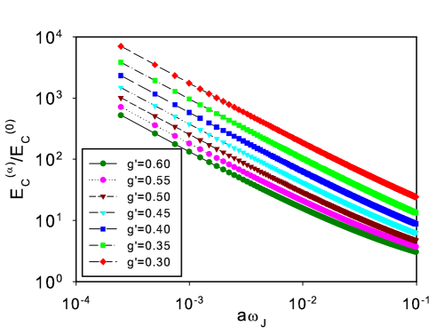
Figure 2: The ratio $E_{C}^{(\alpha)}/E_{C}^{(0)}$ as a function of dimensionless separation $a\omega_{J}$ for different oscillator strength $g^{\prime}=\sqrt{g_{J}}/\omega_{J}$ in the closed surface band gap limit, $m=0$. Where $E_{C}^{(\alpha)}$($E_{C}^{(0)}$) is the Casimir energy with(without) surface correction. Here fermion velocity $v_{F}=1.0\times 10^{-3}$.

In this paper, we analyze Casimir interaction between TIs with finite surface band gap. First, for large surface band gap limit $(m\rightarrow\infty)$, we can obtain same results given in [Phys. Rev. Lett. 106, 020403 (2011)]Grushin_PRL (19) from equations (17)-(21). Second, for small surface band gap limit $(m\rightarrow 0)$, the off-diagonal terms in Fresnel coefficients matrices will vanish and Casimir energy can be rewritten in imaginary time formalism as:

$$\frac{E_{C}(a)}{A} = \int_{0}^{\infty}\frac{{d}k_{0}}{2\pi}\int\frac{d^{2}k_{\parallel}}{(2\pi)^{2}}\left[\log\left(1-e^{-2ka}r_{TE}^{(1)}r_{TE}^{(2)}\right)\right.$$ (22)

$$+\left.\log\left(1-e^{-2ka}r_{TM}^{(1)}r_{TM}^{(2)}\right)\right],$$

with

$$r_{TE} = -1+\frac{2}{1+\frac{p_{3}}{k_{3}}+\frac{\pi\alpha}{4}\sqrt{\cos^{2}\theta+v_{F}^{2}\sin^{2}\theta}},$$ (23)

$$r_{TM} = 1-\frac{2\frac{p_{3}}{k_{3}}\sqrt{\cos^{2}\theta+v_{F}^{2}\sin^{2}\theta}}{\frac{\pi\alpha}{4}\frac{p_{3}}{k_{3}}+(\frac{p_{3}}{k_{3}}+\varepsilon)\sqrt{\cos^{2}\theta+v_{F}^{2}\sin^{2}\theta}},$$ (24)

where $k_{3}=\sqrt{k_{0}^{2}+\bm{k}_{\parallel}^{2}}$, $p_{3}=\sqrt{\varepsilon{k_{0}^{2}}+\bm{k}_{\parallel}^{2}}$, and $\theta=\cos^{-1}(k_{0}/k_{3})$.

The Casimir energy between dielectric materials without special boundary conditions, $\alpha\rightarrow 0$ in Eq.(23) and Eq.(24), has been studiedBordag_book (28, 29, 30).

Considering correction from surface interaction, for large separation limit, we obtain the correction up to first order of fine structure constant:

$$\frac{E_{C}^{(1)}(a)}{E_{0}}=-\frac{\pi\alpha}{4d^{3}}\left[\frac{\varepsilon(0)-1}{(\varepsilon(0)+1)^{3}}\log{\frac{1}{v_{F}}}\right.$$

$$+\left.\frac{\log\left[\frac{1}{2}\left(1+\sqrt{\varepsilon(0)}\right)\right]}{\varepsilon(0)-1}-\frac{3+5\sqrt{\varepsilon(0)}}{4\left(1+\sqrt{\varepsilon(0)}\right)^{3}}\right],$$ (25)

where $E_{0}=A\omega_{J}^{3}/(2\pi)^{2}$ which is set as the unit of Casimir energy, $d=a\omega_{J}$ is the dimensionless separation.

For small separation limit, in order to make the physics more clear, we also formally expand Eq.(22) in powers of $\alpha$, up to first order correction, the Casimir energy takes the following form(here we assume the relative oscillator strength $g_{J}/\omega_{J}^{2}\ll 1$):

$$\frac{E_{C}^{(1)}(a)}{E_{0}} =-\frac{g_{J}}{\omega_{J}^{2}}\frac{\pi\alpha}{64d^{3}}\int_{0}^{\infty}dyy^{2}e^{-y}$$ (26)

$$\left[\frac{\theta(t)}{\sqrt{t}}\text{arctan}\sqrt{t}+\frac{\theta(-t)}{\sqrt{-t}}\text{arctanh}\sqrt{-t}\right],$$

where $t=-1+{v_{F}^{2}y^{2}}/{4d^{2}}$ and $\theta(t)$ is the Heaviside unit step function. Casimir energy is dominated by surface Dirac fermion and turns into the ideal conductor case which is proportional to $1/a^{3}$. This conclusion is also confirmed numerically in Fig.[2].

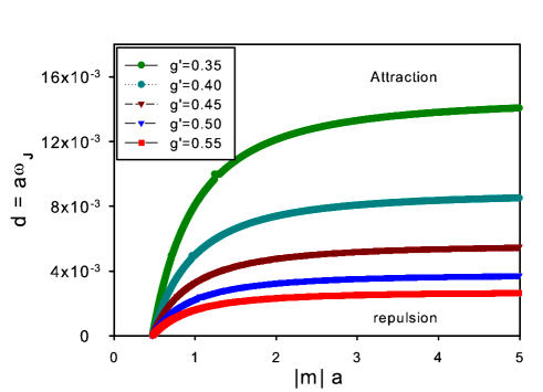
Figure 3: Boundary of repulsive and attractive Casimir interaction in the plane of dimensionless separation $d=a\omega_{J}$ and product $|m|a$ for different oscillator strengths $g^{\prime}=\sqrt{g_{J}}/\omega_{J}$. When the parameters $d$ and $|m|a$ have been taken in the left-up region over these lines, the Casimir interaction is attractive, when $d$ and $|m|a$ have been taken in the lower-right region of these lines, the Casimir interaction is repulsive. (The relative Fermi velocity $v_{F}$ has been taken to be $1.0\times 10^{-3}$).

Finally, for general surface band gap, we have two dimensionless parameters: $m/\omega_{J}$ and $d=\omega_{J}{a}$ (there are two other parameters in our model, the Fermi velocity of surface fermion, $v_{F}$, and optical oscillator strength in TIs, $g_{J}/\omega_{J}^{2}$, which both have quantitatively influence on Casimir energy). For the large separation limit $(a\gg\text{max}(1/\omega_{J},1/|m|))$, we expand the integral in Eq.(20) in power of fine structure constantalpha (31) $\alpha$ and consider the correction up to $\alpha$. In this case, the dielectric permittivity $\varepsilon(ik_{0})$ can be approximated by long wave length limit value $\varepsilon(0)$, and the Casimir energy correction from interaction between surface fermions and electromagnetic field reads:

$$\frac{E_{C}^{(1)}(a)}{E_{0}}=-\frac{|m|\alpha}{\omega_{J}d^{2}}\int_{0}^{1}\frac{dx}{v_{F}^{2}+x^{2}}\left[\frac{r^{2}(\varepsilon(0)-r)}{(\varepsilon(0)+r)^{3}}+\frac{x^{2}(1-r)}{(1+r)^{3}}\right],$$ (27)

where $r=\sqrt{1+(\varepsilon(0)-1)x^{2}}$, and $v_{F}\ll 1$.

For the small separation limit $(d\rightarrow 0)$, in order to make the physics more clear, we also formally expand the Casimir energy in power series of $\alpha$. In this case, the Casimir energy is dominated by surface terms, the term which contains $\tilde{\Phi}^{2}$ and is proportional to $1/m^{2}a^{5}$ is important. However this dominant term will be suppressed if $|m|a\rightarrow\infty$, the topological term which contains $\text{sign}(\theta_{1}\theta_{2})\tilde{\phi}^{2}$ and is proportional to $1/a^{3}$ will provide a large repulsive potential between TIs when $\text{sign}(\theta_{1}\theta_{2})=-1$. So the surface terms in Casimir energy will dominate and $|m|a$ is a good parameter to estimate the Casimir force: when $|m|a\gg 1$, the Casimir force will be repulsive and when $|m|a\ll 1$, the Casimir force will be attractive.

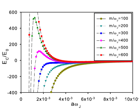
Figure 4: Casimir energy density $E_{C}$ (in units of $E_{0}=\omega_{J}^{2}/(2\pi)^{2}$) as a function of the dimensionless distance $d=a\omega_{J}$ with different surface band gaps $m/\omega_{J}$. Here we take the dimensionless oscillator strength $g_{J}/\omega_{J}^{2}=0.45^{2}$ and Fermi velocity $v_{F}=1.0\times 10^{-3}$.

In Fig.[3], we give the boundary of repulsive and attractive Casimir interaction, as a function of dimensionless separation $d=a\omega_{J}$ and product $|m|a$. We find that there is a critical value $(|m|a)_{c}\sim 1/2$, when $|m|a<(|m|a)_{c}$, the Casimir interaction is attractive for any separation length. The independence of $(|m|a)_{c}$ on oscillator strength $g_{J}/\omega_{J}^{2}$ shows that Casimir interaction, in small separation limit, is dominated by surface terms. More intuitively, we calculated the Casimir energy as a function of dimensionless separation $d=a\omega_{J}$ for different surface band gaps, as shown in Fig.[4], for given parameters, $g_{J}/\omega_{J}^{2}=0.45^{2}$ and $v_{F}=1.0\times 10^{-3}$. We find the critical surface band gap, where the repulsive peak disappears, $m_{c}\approx 300\omega_{J}$ (the blue-square dotted line in Fig.[4]).

We note that our calculations can be generalized to multi-value of topological magnetoelectric polarizability $\theta=(2n+1)\pi$ ($n$ is an integer) straightforward by introducing multi-fermion on TI surface, and the critical value $(|m|a)_{c}$ is independent on the absolute value of $\theta$ (as shown in Fig.[5]), this is because in short separation limit, Casimir interaction is dominated by surface terms and each species fermion will contribute both repulsive and attractive Casimir interaction if $\text{sign}(\theta_{1})=-\text{sign}(\theta_{2})$.

We can use this relationship to estimate the critical surface band gap for repulsive Casimir interaction. For $\text{Tl}\text{Bi}\text{Se}_{2}$ suggested in Ref.Grushin_PRL (19), the minimum of Casimir energy appears at a separation of $a\sim 0.1{\mu}m$, and the corresponding surface band gap needs to be greater than $1eV$, which reflects that the width of surface band gap opened by magnetic coating is non-ignorable and unaccessible experimentally.

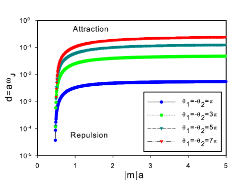
Figure 5: Boundary of repulsive and attractive Casimir interaction in the plane of dimensionless separation $d=a\omega_{J}$ and product $|m|a$ for different topological magnetoelectric polarizability. (The relative Fermi velocity $v_{F}$ and oscillator strength $g_{J}/\omega_{J}^{2}$ has been taken to be $1.0\times 10^{-3}$ and $0.45^{2}$ respectively).

V Conclusion

We studied the Casimir energy between TIs with opposite topological magnetoelectric polarizability and finite surface band gap via Lifshitz formula, we found that, in small separation limit, Casimir force is dominated by interaction between surface fermion and electromagnetic field in the vacuum, and a great surface band gap $m>m_{c}\sim 1/(2a)$ is essential for repulsive Casimir interaction.

*

Appendix A Effective action

We give a detailed derivation of the effective action(3) in this appendix. The effective action from quantum field theory is:

$$S_{eff}(A)=\frac{1}{2}\int\frac{d^{3}k}{(2\pi)^{3}}A_{a}(k)\Pi^{ab}(k)A_{b}(k),$$ (28)

where $\Pi(k)$ is the polarization tensor, which takes the form:

$$i\Pi^{ab}(k)=-e^{2}\int\frac{d^{3}p}{(2\pi)^{3}}\text{tr}[(-i\gamma^{a})G(k+p)(-i\gamma^{b})G(k)],$$ (29)

and $G(k)=i/(\gamma^{a}k_{a}+m)$ is the propagator of fermion on TI surface. From the standard calculation in quantum field theory, one can get the exact form of polarization tensor:

$$\Pi(k) = \Pi_{1}(k)+\Pi_{2}(k)$$ (30)

$$\Pi_{1}^{ab}(k) = \frac{\phi(\lambda)}{4\pi}\epsilon^{abc}ik_{c}$$ (31)

$$\Pi_{2}(k) = \frac{\Phi(\lambda)}{2\pi|m|}\left(\begin{array}[]{ccc}k_{x}^{2}+k_{y}^{2}&-k_{0}k_{x}&-k_{0}k_{y}\\ -k_{0}k_{x}&k_{0}^{2}-v_{F}^{2}k_{y}^{2}&v_{F}^{2}k_{x}k_{y}\\ -k_{0}k_{y}&v_{F}^{2}k_{x}k_{y}&k_{0}^{2}-v_{F}^{2}k_{x}^{2}\end{array}\right)$$ (35)

where $\phi(\lambda)$ and $\Phi(\lambda)$ has been given in Eq.(4) and Eq.(5), $k_{1,2}(k_{0})$ are the momentum(frequency) of electromagnetic field. One can check that the polarization tensor satisfies Ward identity, $\sum_{a}k_{a}\Pi^{ab}(k)=\sum_{b}\Pi^{ab}(k)k_{b}=0$. The Fourier transformation of Eq.(28) gives Eq.(3).
We take $\Pi^{xy}(k)$ as an example to show more detailed calculations of polarization tensor. Taking the trace in Eq.(29), one can get

$$i\Pi^{xy}(k)=-e^{2}\int\frac{d^{3}p}{(2\pi)^{3}}\frac{2v_{F}^{2}[-imk_{0}+v_{F}^{2}(2k_{x}k_{y}+k_{x}p_{y}+k_{y}p_{x})]}{[(p_{0}+k_{0})^{2}+m^{2}-v_{F}^{2}(\bm{p}+\bm{k})^{2}][k_{0}^{2}+m^{2}-v_{F}^{2}\bm{k}^{2}]}.$$ (37)

One can get the following form of $i\Pi^{xy}(k)$ by introducing a Feynman parameter $x$ and redefining the integration variables $l_{a}^{\prime}=p_{a}+xk_{a}$, $l_{0}=l_{0}^{\prime}$, and $\bm{l}=v_{F}\bm{l}^{\prime}$:

$$i\Pi^{xy}(k)=-2e^{2}\int_{0}^{1}dx\int\frac{d^{3}l}{(2\pi)^{3}}\frac{imk_{0}+2x(1-x)v_{F}^{2}k_{x}k_{y}}{\left(l_{0}^{2}-\bm{l}^{2}-\Delta\right)^{2}},$$ (38)

where $\Delta=m^{2}-x(1-x)(k_{0}^{2}-v_{F}^{2}\bm{k}^{2})=m^{2}[1-\lambda x(1-x)]$. Making Wick rotation $l_{0}\rightarrow{il_{0}^{E}}$ and integration over $l$, we find:

$$i\Pi^{xy}(k) = ie^{2}\left[imk_{0}\int\frac{dx}{4\pi\sqrt{\Delta}}+v_{F}^{2}k_{x}k_{y}\int dx\frac{x(1-x)}{2\pi\sqrt{\Delta}}\right]$$ (39)

$$= i\left(\frac{ik_{0}}{4\pi}\phi(\lambda)+\frac{v_{F}^{2}k_{x}k_{y}}{2\pi|m|}\Phi(\lambda)\right)$$

Comparing with the effective action of electromagnetic field in monolayer graphene system as shown in Ref.graphene (32), we find that there is an additional topological term Eq.(31) together with the normal vacuum polarization Eq.(35), the first term is essential for TI because this parity-odd term reflects the fact that there are always odd species of surface fermions which are spin-momentum locked, the contribution from second term is analogy to Dirac fermion in monolayer graphene system and reflects the dynamical response of TI surface state to extra electromagnetic field.

References

(1)
X. L. Qi and S. C. Zhang,
Phys. Today63,
33 (2010).
(2)
J. E. Moore,
Nature464,
194 (2010).
(3)
M. Z. Hasan, and C. L. Kane,
Rev. Mor. Phys.82,
3045 (2010).
(4)
D. Hsieh, D. Qian, L. Wray, Y. Xia, Y. S. Hor, R. J. Cava, and M. Z. Hasan,
Nature452,
970 (2008).
(5)
Y. L. Chen, J. G. Analytis, J.-H. Chu, Z. K. Liu, S.-K. Mo, X. L. Qi, H. J. Zhang,
D. H. Lu, X. Dai, Z. Fang, S. C. Zhang, I. R. Fisher, Z. Hussain, and Z.-X. Shen,
Science325,
178 (2009).
(6)
Y. Xia, D. Qian, D. Hsieh, L. Wray, A. Pal, H. Lin, A. Bansil, D. Grauer,
Y. S. Hor, R. J. Cava, and M. Z. Hasan,
Nature Physics5,
398 (2009).
(7)
D. Hsieh, Y. Xia, D. Qian, L. Wray, J. H. Dil, F. Meier, J. Osterwalder, L. Patthey, J. G. Checkelsky,
N. P. Ong, A. V. Fedorov, H. Lin, A. Bansil, D. Grauer, Y. S. Hor, R. J. Cava, and M. Z. Hasan,
Nature460,
1101 (2008).
(8)
D. Hsieh, Y. Xia, D. Qian, L. Wray, F. Meier, J. H. Dil, J. Osterwalder,
L. Patthey, A. V. Fedorov, H. Lin, A. Bansil, D. Grauer, Y. S. Hor, R. J. Cava, and M. Z. Hasan,
Phys. Rev. Lett.103,
146401 (2009).
(9)
Y. L. Chen, J.-H. Chu, J. G. Analytis, Z. K. Liu, K. Igarashi, H.-H. Kuo, X. L. Qi,
S. K. Mo, R. G. Moore, D. H. Lu, M. Hashimoto, T. Sasagawa, S. C. Zhang, I. R. Fisher, Z. Hussain, and Z. X. Shen,
Science329,
659 (2010).
(10)
L. Fu, C. L. Kane, and E. J. Mele,
Phys. Rev. Lett.98,
106803 (2007).
(11)
L. Fu and C. L. Kane,
Phys. Rev. B76,
045302 (2007).
(12)
J. E. Moore and L. Balents,
Phys. Rev. B75,
121306(R) (2007).
(13)
X. L. Qi, T. L. Hughes, and S. C. Zhang,
Phys. Rev. B78,
195424 (2008).
(14)
B. A. Bernevig, T. L. Hughes, and S. C. Zhang,
Science314,
1757 (2006).
(15)
M. König, S. Wiedmann, C. Brüne, A. Roth, H. Buhmann,
L. W. Molenkamp, X. L. Qi, and S. C. Zhang,
Science318,
766 (2007).
(16)
H. Zhang, C.-X. Liu, X. L. Qi, X. Dai, Z. Fang, and S. C. Zhang,
Nature Physics5,
438 (2009).
(17)
X. L. Qi, R. Li, J. Zang, and S. C. Zhang,
Science323,
1184 (2009).
(18)
L. Fu and C. L. Kane,
Phys. Rev. Lett.100,
096407 (2008).
(19)
A. G. Grushin, and A. Cortijo,
Phys. Rev. Lett.106,
020403 (2011).
(20)
A. G. Grushin, P. Rodriguez-Lopez, and A. Cortijo,
e-print arXiv:cond-mat1102.0455 (2011).
(21)
M. Levin, A. P. McCauley, A. W. Rodriguez, M. T. H. Reid, and S. G. Johnson,
Phys. Rev. Lett.105,
090403 (2010).
(22)
R. Zhao, J. Zhou, T. Koschny, E. N. Economou, and C. M. Soukoulis,
Phys. Rev. Lett.103,
103602 (2009).
(23)
P. J. van Zwol, and G. Palasantzas,
Phys. Rev. A81,
062502 (2010).
(24)
J. Chay, D. K. Hong, T. Lee, and S. H. Park,
Phys. Rev. D48,
909 (1993).
(25)
D. K. Kim, and K.-S. Soh,
Phys. Rev. D55,
6218 (1997).
(26)
J. Novotný,
Mod. Phys. Lett.A7,
2575 (2002).
(27)
A. Karch,
Phys. Rev. Lett.103,
171601 (2009).
(28)
M. Bordag, G. L. Klimchitskaya, U. Mohideen, and V. M. Mostepanenko,
”Advances in the Casimir Effect”,
(Oxford University Press, Oxford, 2009).
(29)
M. Bordag, U. Mohideen, and V. M. Mostepanenko,
Phys. Rep.353,
1 (2001).
(30)
A. Lambrecht, P. A M. Neto, and S. Reynaud,
New Journal of Physics8,
243 (2006).
(31)
We note that we do not expand the integral in power of , the reason is, in short separation limit
integration over momentum will give a divergence which set the term proportional to large than next
to leading order term or even the leading order term (in large surface band gap limit), this divergence is supressed
in large separation limit.
(32)
M.Bordag, I. V. Fialkovsky, D, M. Gitman, and D. V. Vassilevich,
Phy. Rev. B80,
245406(2009).