ESO 546-G34: The most metal poor LSB galaxy?

Abstract

We present a re-analysis of spectroscopic data for 23 H ii-regions in 12 blue, metal-poor low surface brightness galaxies (LSBGs) taking advantage of recent developments in calibrating strong-line methods. In doing so we have identified a galaxy (ESO 546-G34) which may be the most metal-poor LSB galaxy found in the local Universe. Furthermore, we see evidence that blue metal-poor LSBGs, together with blue compact galaxies (BCGs) and many other H ii galaxies, fall outside the regular luminosity-metallicity relation. This suggests there might be an evolutionary connection between LSBGs and BCGs. In such case, several very metal-poor LSBGs should exist in the local Universe.

1 Introduction

Among blue metal-poor low surface brightness galaxies (LSBGs) one may very well find the most unevolved objects in the low-$z$ Universe (Bothun et al., 1990; Lacey & Silk, 1991). LSBGs investigated by Rönnback & Bergvall (1994, 1995) as well as those studied by de Blok, McGaugh & van der Hulst (1996) tend to be bluer than most other galaxies of the same type. However, the wide range of colours and metallicities, from very blue and metal-poor to very red and relatively metal-rich, suggests that LSBGs also have a wide range of evolutionary states, just like their high surface brightness (HSB) counterparts (Mattsson, Caldwell & Bergvall, 2008; Liang et al., 2010). It is then natural to assume that blue LSB galaxies are young and unevolved and red LSB galaxies are old and evolved, especially since the blue ones appear metal poor and the red ones quite metal rich (McGaugh, 1994; Kuzio de Naray, McGaugh & de Blok, 2004).

A simple and attractive explanation for the LSB property is that LSBGs are simply forming stars very inefficiently (Bothun et al., 1990; Boissier, 2008). This inefficiency may reflect lower star-formation rates in the star-forming regions in general, or a star formation threshold leading to fewer star-forming regions, i.e., a lower star formation density in total (see, e.g., Kennicutt, 1989; van der Hulst et al., 1993). This picture is also very much consistent with the rather high gas mass fractions found in LSBGs (see, e.g. Kuzio de Naray, McGaugh & de Blok, 2004, and references therein). If this hypothesis for the LSB property holds true, a direct consequence would be that blue LSBGs are very unevolved objects and some of them may have extremely low metallicities.

It is often difficult to detect the ${\rm[O~{}\textsc{iii}]}\lambda 4363$-line in LSBGs and hence impossible to use a ’direct’ method (based on the electron temperature $T_{\rm e}$) to derive abundances. This suggests there might exist extremely metal-poor LSBGs which have not been labelled as such, since a $T_{\rm e}$-based method could not be used and existing strong-line calibrations are not made for the very metal-poor regime or at best give very uncertain results.

In this letter we reanalyse, in the light of recent developments in calibrating strong-line methods of high-precision (Pilyugin & Mattsson, 2011; Pilyugin, Vílchez & Thuan, 2010), a sample of blue unevolved LSBGs observed spectroscopically by Rönnback & Bergvall (1995). Our results indicate that one of the expected extremely metal-poor LSBGs is present in our sample. We also compare the rederived LSBG abundances to the abundances of metal-poor BCGs and H ii galaxies

Table 1: Strong-line indices and H$\beta$ fluxes for the 23 H ii-regions in this study.

Object	$R_{2}$	$R_{3}$	$N_{2}$	$S_{2}$	I(H$\beta)\cdot 10^{19}$
					[W m-2]
146G14B	2.23	3.52	0.146	0.430	6.59
146G14C	3.26	3.56	0.200	0.620	21.0
489G56A	0.74	4.51	0.044	0.138	5.90
489G56B	1.26	1.88	0.106	0.295	2.44
505G04A	3.06	2.90	0.153	0.523	9.13
505G04B	2.89	3.06	0.170	0.498	8.89
546G34A	1.79	2.20	0.062	0.304	3.83
546G34B	1.81	1.45	0.069	0.286	2.82
462G22	2.94	2.71	0.203	0.588	1.36
546G09	2.25	4.00	0.189	0.483	8.12
158G15A	2.13	6.16	0.124	0.305	104
158G15B	3.92	3.67	0.062	0.506	32.4
359G31A	2.79	3.38	0.252	0.646	1.55
359G31B	3.27	2.67	0.323	0.655	8.35
576G59A	2.35	4.33	0.165	0.361	13.2
576G59B	1.76	5.04	0.105	0.396	11.9
114G07A	1.19	6.79	0.086	0.234	107
114G07C	1.29	6.82	0.070	0.229	43.6
405G06A	3.45	2.90	0.244	0.730	6.88
405G06B	4.00	2.40	0.265	0.647	1.43
405G06C	1.85	6.21	0.093	0.238	5.36
504G10A	3.10	3.02	0.291	0.721	1.32
504G10B	2.25	4.92	0.174	0.402	2.83

2 Abundance derivations

Abundances are derived either ’directly’ by estimating the electron temperature from oxygen emission lines and then computing abundance ratios from the relative strength of the corresponding emission lines together with correction factors for the degree of ionisation, or by using calibrated relations between strong-line fluxes and atomic abundances. When describing the methods below, and in further discussions in this paper, we will be using the following notations for the strong-line indices,

$$R = [{\rm O}~{}\textsc{iii}]\lambda 4363=I_{[\rm O~{}\textsc{iii}]\lambda 4363}/I_{{\rm H}\beta},$$

$$R_{2} = [{\rm O}~{}\textsc{ii}]\lambda 3727+\lambda 3729=I_{\rm[O~{}\textsc{ii}]\lambda 3727+\lambda 3729}/I_{{\rm H}\beta},$$

$$N_{2} = [{\rm N}~{}\textsc{ii}]\lambda 6548+\lambda 6584=I_{\rm[N~{}\textsc{ii}]\lambda 6548+\lambda 6584}/I_{{\rm H}\beta},$$ (1)

$$S_{2} = [{\rm S}~{}\textsc{ii}]\lambda 6717+\lambda 6731=I_{\rm[S~{}\textsc{ii}]\lambda 6717+\lambda 6731}/I_{{\rm H}\beta},$$

$$R_{3} = [{\rm O}~{}\textsc{iii}]\lambda 4959+\lambda 5007=I_{{\rm[O~{}\textsc{iii}]}\lambda 4959+\lambda 5007}/I_{{\rm H}\beta}.$$

We derive abundances for 23 H ii-regions in LSBGs from the Rönnback & Bergvall (1995) LSBG sample where sulfur and nitrogen lines were detected. The $N_{2}$ and $S_{2}$ indices (see Table 1) can then be used to estimate abundances and electron temperatures. We use the ’NS-calibration’ by Pilyugin & Mattsson (2011) and the ’ON-calibration’ by Pilyugin, Vílchez & Thuan (2010). More precisely, we derive abundances using relations of the form

$$12+\log{\rm\left({X\over H}\right)}_{\rm NS}=a_{0}+a_{1}\,\log R_{3}+a_{2}\,\log N_{2}+a_{3}\,\log\left({N_{2}\over S_{2}}\right),$$ (2)

and

$$12+\log{\rm\left({X\over H}\right)}_{\rm ON}=a_{0}+a_{1}\,\log R_{3}+a_{2}\,\log R_{2}+a_{3}\,\log\left({N_{2}\over R_{2}}\right),$$ (3)

respectively, where the coefficients $a_{i}$ are fitting parameters obtained using a ”calibration sample” of local galaxies with well-measured $T_{\rm e}$-based abundances in their H ii-regions (see Pilyugin, Vílchez & Thuan, 2010; Pilyugin & Mattsson, 2011, for further details). Both the NS- and the ON-calibrations avoid the often weak ${\rm[O~{}\textsc{III}]}\lambda 4363$-line, and in the case of the NS-calibration also the ${\rm[O~{}\textsc{II}]\lambda 3727+\lambda 3729}$-lines, which are sometimes uncertain in LSBGs (combining all relevant uncertainties one finds that the $R_{2}$-index may have a $\pm 20$% uncertainty). Whenever possible, we also derive ’direct’ $T_{\rm e}$-based abundances according to Pilyugin, Vílchez & Thuan (2010).

The NS-calibration uses the $N_{2}$ and $S_{2}$ indices as a kind of ’substitute’ for the electron temperature and the ionisation factor, while the ON-calibration uses the $N_{2}$ and $R_{2}$ indices. However, the $R_{2}$ index is sometimes hard to determine in LSBGs. Two such examples are ESO 489-G56 and ESO 546-G34 Rönnback & Bergvall (see Fig. 2 in 1995) which are both most likely a very metal poor LSB galaxies. Using a calibration without $R_{2}$, such as the NS-calibration, is therefore important to get a good handle on the abundances in some objects. This is especially true for the N/O ratio.

For a smaller number (13) of H ii-regions where the ${\rm[O~{}\textsc{III}]}\lambda 4363$-line can be detected, we can also derive electron temperatures $T_{\rm e}$ and corresponding $T_{\rm e}$-based abundances. More precisely, the O⁺- and O⁺⁺-zone temperatures, $t_{3}$ and $t_{2}$, are obtained iteratively using recent calibrations by Pilyugin, Vílchez & Thuan (2010) based on the principles described in Pilyugin et al. (2009), i.e.,

$$t_{3}={1.467\over\log\left({R_{3}/R}\right)-0.876-0.193\log(t_{3})+0.033\,t_{3}}$$ (4)

and

$$t_{2}=0.314+0.672\,t_{3},$$ (5)

where $t_{3}$ and $t_{2}$ are given in units of 10⁴K. The oxygen and nitrogen abundances can then be calculated from

$$\log\left({{\rm O}\over{\rm H}}\right)=\log({\rm O}_{3}+{\rm O}_{2}),$$ (6)

where

$$\log({\rm O}_{2})=\log(R_{2})+5.929+{1.617\over t_{2}}-0.568\log(t_{2})-0.008\,t_{2}$$ (7)

$$\log({\rm O}_{3})=\log(R_{3})+6.251+{1.204\over t_{3}}-0.613\log(t_{3})-0.015\,t_{3},$$ (8)

and

$$\log\left({\rm{N}\over\rm{O}}\right)=\log\left({N_{2}\over R_{2}}\right)+0.334-{0.724\over t_{2}}-0.035\log(t_{2})+0.005\,t_{2}.$$ (9)

The emission line data taken from Rönnback & Bergvall (1995) has been corrected for extinction and, more importantly, absorption features due to the underlying stellar population. The underlying absorption in the Balmer lines is tightly correlated with the strength of the 4000Å-break (Mattsson & Bergvall, 2009). In terms of the $D(4000)$-parameter (Bruzual, 1983) the underlying absorption has a maximum just above $D(4000)=1$ (no or weak discontinuity). We find that all 23 H ii-regions considered in the present study have $D(4000)$ close to unity and thus significant underlying absorption in H$\alpha$ and H$\beta$ is expected. Quantitatively, this means the correction is around 3Å in the equivalent width of H$\alpha$ and 5Å in H$\beta$. We chose to keep the original corrections (listed in Table 2) made by Rönnback & Bergvall (1995) since reanalysis of a few objects (ESO 146-G14, ESO 158-G15 and ESO 546-G34) gave essentially the same result and the grid of SEMs used by Rönnback & Bergvall (1995) covers a larger part of parameter space. The software used for applying the original corrections was in itself corrected after Rönnback & Bergvall (1995) had published their results. Hence, the numbers presented here differ slightly from those in Rönnback & Bergvall (1995) in some cases.

Table 2: Derived abundances, using the notations ${\rm O/H}=12+\log({\rm O/H})$ and ${\rm N/O}=\log({\rm N/O})$ for brevity, and corrections for underlying absorption ($W_{\rm abs}$) in Ångströms for the 23 H ii-regions. All numbers are based on data from Rönnback & Bergvall (1995), except for ESO 146-G14 where data are taken from Bergvall & Rönnback (1995). $R_{23}$-abundances are according to Rönnback & Bergvall (1995) using the calibration by McGaugh (1994).

Object	$({\rm O/H})_{\rm NS}$	$({\rm O/H})_{\rm ON}$	$({\rm O/H})_{T_{\rm e}}$	$({\rm O/H})_{T_{\rm e}}^{\rm RB95}$	$({\rm O/H})_{R_{23}}$	$({\rm N/O})_{\rm NS}$	$({\rm N/O})_{\rm ON}$	$({\rm N/O})_{T_{\rm e}}$	$({\rm N/O})_{T_{\rm e}}{\rm RB95}$	$W_{\rm abs}({\rm H}\alpha)$	$W_{\rm abs}({\rm H}\beta)$
146G14B	7.83	7.83	7.69	7.59	8.02	-1.48	-1.42	-1.38	-1.51	5.0	6.5
146G14C	7.93	7.91	7.60	7.54	-	-1.48	-1.46	-	-	4.2	4.8
489G56A	7.59	7.60	7.47	7.49	7.63	-1.50	-1.41	-1.37	-1.35	4.0	4.8
489G56B	7.49	7.52	-	-	7.52	-1.46	-1.30	-	-	4.2	6.3
505G04A	7.77	7.75	7.68	7.63	8.03	-1.50	-1.52	-1.48	-1.44	4.7	5.8
505G04B	7.82	7.81	7.82	7.77	8.01	-1.47	-1.47	-1.47	-1.43	4.5	5.6
546G34A	7.40	7.38	-	-	7.69	-1.55	-1.60	-	-	4.9	6.6
546G34B	7.26	7.25	-	-	7.64	-1.52	-1.56	-	-	3.3	4.6
462G22	7.82	7.82	-	-	7.99	-1.47	-1.41	-	-	4.5	6.6
546G09	7.96	7.96	-	-	7.97	-1.46	-1.35	-	-	2.6	2.7
158G15A	8.02	8.00	8.10	8.07	8.14	-1.46	-1.47	-1.53	-1.49	1.8	3.8
158G15B	7.60	7.53	-	-	8.24	-1.64	-1.89	-	-	3.7	4.5
359G31A	7.97	7.98	-	-	8.05	-1.45	-1.33	-	-	3.2	4.0
359G31B	7.95	7.95	-	-	8.05	-1.41	-1.31	-	-	3.8	4.7
576G59A	7.96	7.95	8.14	8.09	8.02	-1.44	-1.41	-1.49	-1.46	3.1	3.3
576G59B	7.88	7.88	7.77	7.81	8.00	-1.52	-1.45	-1.43	-1.47	2.9	3.0
114G07A	7.95	7.95	8.01	8.04	8.00	-1.48	-1.38	-1.42	-1.41	2.7	3.0
114G07C	7.89	7.89	8.05	8.03	8.04	-1.51	-1.47	-1.55	-1.52	2.8	3.2
405G06A	7.90	7.89	7.89	7.83	8.10	-1.47	-1.42	-1.40	-1.36	4.1	5.1
405G06B	7.85	7.83	-	-	8.16	-1.44	-1.44	-	-	2.9	3.7
405G06C	7.94	7.92	8.14	8.11	8.09	-1.47	-1.51	-1.61	-1.59	2.6	2.8
504G10A	7.97	7.97	-	-	8.12	-1.45	-1.32	-	-	3.9	5.5
504G10B	8.02	8.02	8.14	8.11	8.05	-1.45	-1.38	-1.44	-1.44	5.7	7.3

3 Results and discussion

3.1 Abundances

The full set of derived abundances, together with the original numbers derived by Rönnback & Bergvall (1995), is presented in Table 2. We estimate the typical error (mainly due to the method itself) in abundances derived using the NS- and ON-calibrations to be $\pm 0.1$ dex, and the $T_{\rm e}$-based abundances is expected to have slightly smaller total errors. The typical relative mean errors of the line intensities are 5-10%, which makes the strong-line calibration itself the dominant source of uncertainty. However, we would like to point out a caveat to the [N ii]-fluxes in general: the resolution of the Rönnback & Bergvall (1995) spectra are not high enough to resolve the [N ii]- and H$\alpha$-line in a satisfactory way. This may add further uncertainty to the line fluxes (see the detailed discussion about ESO 546-G34 below) and typically lead to overestimated $N_{2}$-indices.

The $T_{\rm e}$-based abundances agree very well with the abundances derived by Rönnback & Bergvall (1995, see also Figs. 1 and 2 in the present paper). Among the galaxies with detectable ${\rm[O~{}{\textsc{I}II}]}\lambda 4363$-lines, the lowest $T_{\rm e}$-based oxygen abundance is found in ESO 489-G56 where $12+\log({\rm O/H})=7.47$ (7.49 according to Rönnback & Bergvall, 1995). In fact, we have only been able to find one LSBG with lower $T_{\rm e}$-based oxygen abundance when searching the literature (CGCG 269-049, $\log({\rm O/H})+12=7.43$, Kniazev et al., 2003).

The ON-abundances also agree with the $T_{\rm e}$-based abundances as well as with the NS-abundances and the existence of a N/O-plateu at low metallicity (see Fig. 2). There is essentially only one exception: H ii region B in ESO 158-G15 which has a significantly lower N/O-ratio than the rest of the sample when using the ON-calibration. This may partly be due to the fact that the $N_{2}$-value for this object lies on the boundary between the cool and warm regimes in the NS- and ON-calibrations, but also that the $N_{2}/R_{2}$-ratio is clearly lower than for the rest of the sample (see Table 1). Among the oxygen abundances derived using the NS- and ON-calibrations we find one particular H ii region with a very low abundance. This is discussed in detail below.

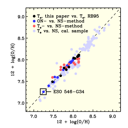
Figure 1: Comparison of oxygen abundances derived using different methods and calibrations. The agreement between the abundances is typically within 0.1 dex with only a few exeptions.

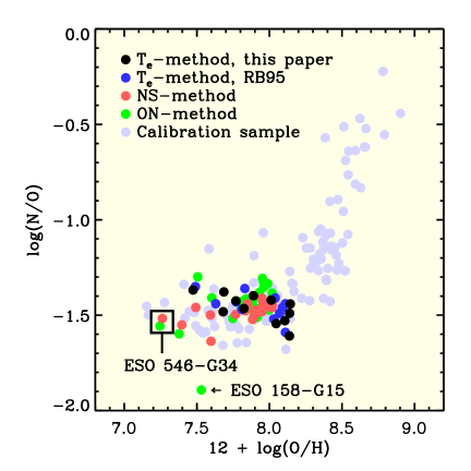
Figure 2: N/O-O/H relation as derived using different methods and calibrations. The deviating object is H ii region B in ESO 158-G15.

3.2 ESO 546-G34

Among the galaxies in this study, ESO 546-G34 stands out as the most metal poor according to our analysis ($\log({\rm O/H})_{\rm NS}+12=7.26,7.40$ and $\log({\rm O/H})_{\rm ON}+12=7.25,7.38$ for the two H ii-regions, respectively). This galaxy is a local (redshift $z=0.00523$) dwarf galaxy of Magellanic type, which has an absolute $B$-band magnitude of $M_{B}=-15.7$, a central surface brightness $\mu_{0,\rm B}=22.9$ and $B-V=0.38$ (Rönnback & Bergvall, 1994). The H i mass is estimated to be $5.4\cdot 10^{8}M_{\odot}$ and the total baryon mass is roughly $1.1\cdot 10^{9}M_{\odot}$ (previously unpublished data, to be presented in more detail in a forthcoming publication). Previous empirical estimates of the oxygen abundances in two of the three observed H ii-regions were significantly higher (Rönnback & Bergvall, 1995), which was likely due to use of ill-determined strong-line calibrations (not suitable for very low metallicities). However, it was noted that the Skillman (1989) calibration derived for metal-poor systems gave $\log({\rm O/H})+12=7.26$ for one of the two detected H ii regions (Bergvall & Rönnback, unpublished), which is essentially the same value we derive using both the NS- and the ON-calibration (see above and Table 2). This places ESO 546-G34 among the very most metal poor galaxies known. ESO 546-G34 may thus be the most metal-poor LSBG ever observed.

ESO 546-G34 show strong oxygen lines relative to other emission lines, which may be a sign of significant shock heating of the interstellar gas. Rönnback & Bergvall (1995) estimated that the shock contribution to H$\beta$ in ESO 546-G34 is very significant - about $20\%$. But they also concluded that the corrections were only minor in most cases and therefore did not include any corrections for shock contributions in their abundance derivations. This does not seem to be appropriate for ESO 546-G34, however. Using a set of shock models (see Rönnback & Bergvall, 1995, and references therein) we confirm that the best fit to the spectra is obtained for a shock contribution to H$\beta$ of $\sim 20\%$. Consequently, we find very strong shock contributions to other lines, e.g., $R_{3}$ has a 70-75% contribution from shocks. This is indeed more than expected, but our preliminary analysis shows that excluding shocks leads to a much worse fit. Taken at face value, the corrections imply that the oxygen abundance in both H ii-regions is $\log({\rm O/H})+12<7.0$, i.e., less than the extreme values of IZw 18 (see Kunth & Östlin, 2000; Östlin, 2000, and references therein), DDO 68 and SBS 0335-052W (Izotov & Thuan, 2007). On the other hand, shock contributions to the line fluxes may increase the inferred electron temperature, which in principle could lead to higher abundances (after correction) when using the direct method. Hence, shock corrections can lead to both a lower or a higher abundance depending on the method/calibration used for deriving it. It is therefore unclear what the effect of shock contributions is in the present case, although it seems most likely the abundances will be corrected downwards.

In the spectra obtained by Rönnback & Bergvall (1995) the $[{\rm N~{}\textsc{ii}}]$- and H$\alpha$-lines cannot be resolved as individual lines. Hence, there is a potential risk that the $N_{2}$-index is underestimated. We have therefore measured the $[{\rm N~{}\textsc{ii}}]$- and $[{\rm S~{}\textsc{ii}}]$-lines in the high resolution VLT/FORS2 spectra obtained by Zackrisson et al. (2006), covering the spectral region around H$\alpha$ (5750-7310Å). It appears the $[{\rm N~{}\textsc{ii}}]$-line flux relative to H$\beta$ may be slightly underestimated (the H$\alpha$-flux would hence be overestimated) in the study by Rönnback & Bergvall (1995), but the data are still consistent within the uncertainties. For the $[{\rm S~{}\textsc{ii}}]$-lines there is good agreement, however. The $N_{2}$-index is about 30% higher in the VLT observations compared to the same in the old data. If this is all due to line blending, then $\log({\rm O/H})_{\rm NS}+12=7.34$ and $\log({\rm O/H})_{\rm ON}+12=7.33$ for region B, and $\log({\rm O/H})_{\rm NS}+12=7.47$ and $\log({\rm O/H})_{\rm ON}+12=7.46$ for region A (not including any effects of shock heating). We cannot rule out the possibility that this may suggest slightly higher abundances, but to be certain new high-resolution spectra (over the whole relevant wavelength range) are needed. Nonetheless, the abundances derived here for ESO 546-G34 are under all circumstances unusually low and it is very unlikely that better data will make these numbers increase significantly.

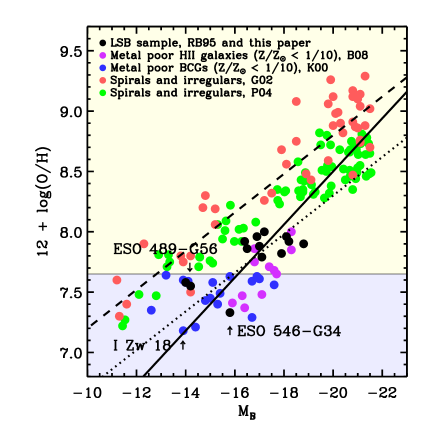
Figure 3: Luminosity-metallicity relation for various types of galaxies. LSBGs and BCGs seem to fall outside ($\sim 0.5$ dex below in oxygen abundance) the relation for spiral and irregular galaxies. The filled black circles show the LSBG sample with mean oxygen abundances obtained using the NS-calibration and B-band magnitudes taken from RB95, while the purple and blue filled circles show metal-poor BCGs and H ii galaxies taken from the literature. The full line is a fit to the LSBGs and spiral galaxies (green circles with $M_{B}$ brighter than $-17$) from Pilyugin, Vílchez & Contini (2004). The dashed line shows the fit to the spiral and irregular galaxies derived by Garnett (2002, red circles); the dotted line show the same relation scaled down by 0.5 dex. Objects falling on the blue-shaded area have metallicities below 1/10 of solar ($12+\log({\rm O/H})\leq 7.65$), usually referred to as the extremely metal-poor regime.

3.3 Luminosity-metallicity relation and the BCG-LSBG connection

BCGs (or H ii galaxies in general) may be triggered by mergers involving gas-rich galaxies with little star formation, e.g., LSBGs Bergvall et al. (1999, 2000); Taylor et al. (1996); Taylor (1997). In Fig. 3 we show the oxygen abundances we derive for the LSBGs using the NS-method in a O/H vs. absolute B-magnitude diagram. Very metal-poor galaxies and LSBGs appear to fall below the usual luminosity-metallicity trend for spiral and irregular galaxies. For similar magnitudes $\log({\rm O/H})$ is typically 0.5 dex lower in our LSBG sample as well as in very metal-poor BCGs (data taken from Kunth & Östlin, 2000) and the H ii sample by Brown, Kewley & Geller (2008). This may lend support to the idea of an evolutionary connection between LSBGs and BCGs, although the data is also consistent with a single relation with large scatter.

In case LSBGs and BCGs fall outside the regular luminosity-metallicity relation, and there is an evolutionary connection between LSBGs and BCGs, what would this connection be? A most likely scenario is the one where BCGs are the result of a major merger between a blue LSB galaxy and another (but evolved) galaxy of similar size, possibly a dwarf elliptical, thus triggering a starburst (Bergvall et al., 1999). This hypotheses naturally explains the LSB component detected in many BCGs (see, e.g. Bergvall & Östlin, 2002) and the similarities in the colours between BCGs and blue LSBGs (Telles & Terlevich, 1997). Moreover, it also have an interesting implication: if there are very metal-poor BCGs, there should be equally (or more) metal-poor LSBGs to be found.

4 Conclusions

We have reanalysed spectroscopic data for 23 H ii-regions in blue, metal-poor LSBGs taking advantage of recent advances in calibrating strong-line methods by Pilyugin, Vílchez & Thuan (2010) and Pilyugin & Mattsson (2011). We have identified a galaxy (ESO 546-G34) which may be the most metal-poor LSB galaxy in the local Universe. We are reasonably sure this is an extremely metal-poor galaxy, although it would be necessary to confirm the abundances using ’direct’ methods, i.e., $T_{\rm e}$-based abundance determinations. For this to be possible ESO 546-G34 needs to be re-observed with better signal-to-noise, which is something we hope to be able to return to.

Finally, we think there is now evidence that blue metal-poor LSBGs, together with many BCGs and H ii galaxies, fall outside the regular luminosty-metallicity relation. This suggests there might be an evolutionary connection between LSBGs and BCGs to be found, as suggested by Bergvall et al. (1999, 2000). In such a case, there should be several very metal-poor LSBGs in the local Universe. We would hence like to encourage the community to search for such candidates.

References

- Bergvall & Rönnback (1995) Bergvall N. & Rönnback J., 1995, MNRAS, 273, 603
- Bergvall et al. (1999) Bergvall N., Östlin G., Masegosa J. & Zackrisson E., 1999, ApSS, 269, 625
- Bergvall et al. (2000) Bergvall N., Masegosa J., Östlin G., & Cernicharo J., 2000, A&A, 359, 41
- Bergvall & Östlin (2002) Bergvall N. & Östlin G., 2002, A&A, 390, 891
- Boissier (2008) Boissier S., Gil de Paz A., Boselli1 A., et al., 2008, ApJ, 681, 244
- Bothun et al. (1990) Bothun G. D., Schombert J. M., Impey C. D. & Schneider S. E., 1990, ApJ, 360, 427
- Brown, Kewley & Geller (2008) Brown W. R., Kewley L. J. & Geller M. J., 2008, AJ, 135, 92 (B08)
- Bruzual (1983) Bruzual A. G., 1983, ApJ, 273, 105
- Bruzual & Charlot (2003) Bruzual A. G. & Charlot S., 2003, MNRAS, 344, 1000
- de Blok, McGaugh & van der Hulst (1996) de Blok W. J. G., McGaugh S. S., & van der Hulst J. M., 1996, MNRAS, 283, 18
- Izotov & Thuan (2007) Izotov Y. & Thuan T. X., 2007, ApJ, 665, 1115
- Kennicutt (1989) Kennicutt R. C., 1989, ApJ, 344, 685
- Kniazev et al. (2003) Kniazev A. Y., Grebel E. K., Hao L., et al., 2003, ApJL, 593, 73
- Kunth & Östlin (2000) Kunth & Östlin G., 2000, ARAA, 10, 1 (K00)
- Kuzio de Naray, McGaugh & de Blok (2004) Kuzio de Naray R., McGaugh S. S. & de Blok W. J. G., 2004, MNRAS, 355, 887
- Lacey & Silk (1991) Lacey C. & Silk J., 1991, ApJ, 381, 14
- Liang et al. (2010) Liang Y. C., Zhong G. H., Hammer F., et al., 2010, MNRAS, 409, 213
- Garnett (2002) Garnett, D.R., 2002, ApJ, 581, 1019 (G02)
- Mattsson & Bergvall (2009) Mattsson L. & Bergvall N., 2009, IAUS, 254, 44
- Mattsson, Caldwell & Bergvall (2008) Mattsson L., Caldwell B. & Bergvall N., 2008, ASPC, 396, 155
- McGaugh (1994) McGaugh S. S., 1994, ApJ, 426, 135
- Pilyugin, Vílchez & Contini (2004) Pilyugin L. S., Vílchez J. M. & Contini T., 2004, A&A, 425, 849 (P04)
- Pilyugin et al. (2009) Pilyugin L. S., Mattsson L., Vílchez J. M. & Cedrés B., 2009, MNRAS, 398, 485
- Pilyugin, Vílchez & Thuan (2010) Pilyugin L. S., Vílchez J. M. & Thuan T. X., 2010, ApJ, 720, 1738
- Pilyugin & Mattsson (2011) Pilyugin L.S. & Mattsson L., 2011, to appear in MNRAS.
- Rönnback & Bergvall (1994) Rönnback J. & Bergvall N., 1994, A&AS, 108, 193
- Rönnback & Bergvall (1995) Rönnback J. & Bergvall N., 1995, A&A, 302, 353 (RB95)
- Skillman (1989) Skillman E. D., 1989, ApJ, 347, 883
- Taylor et al. (1996) Taylor C. L., Thomas D. L., Brinks E. & Skillman E. D., 1996, ApJS, 107, 143
- Taylor (1997) Taylor C.L., 1997, ApJ, 480, 524
- Telles & Terlevich (1997) Telles E. & Terlevich R., 1997, MNRAS, 286, 183
- van der Hulst et al. (1993) van der Hulst, J. M., Skillman, E. D., Smith, T. R., Bothun, G. D., McGaugh, S. S. & de Blok, W. J. G., 1993, AJ, 106, 548
- Zackrisson et al. (2006) Zackrisson E., Bergvall N., Marquart T. & Östlin G., 2006, A&A, 452, 857
- Östlin (2000) Östlin G., 2000, ApJ 535, L99