On the search of sterile neutrinos by oscillometry measurements

Abstract

It is shown that the “new” neutrino with a high mass squared difference and a small mixing angle should reveal itself in the oscillometry measurements. For a judicious monochromatic neutrino source the “new” oscillation length $L_{42}$ is expected shorter than 1.5 m. Thus the needed measurements can be implemented with a gaseous spherical TPC of modest dimensions with a very good energy and position resolution. The best candidates for oscillometry are discussed and the sensitivity to the mixing angle $\theta_{14}$ has been estimated: $\sin^{2}{(2\theta_{14})}$=0.05 (99%) for two months of data handling with ⁵¹Cr.

A recent analysis of the Low Energy Neutrino Anomaly (LNA) RNA ,Giunti and Laveder (2010) led to a challenging claim that this anomaly can be explained in terms of a new fourth neutrino with a much larger mass squared difference. Assuming that the neutrino mass eigenstates are non degenerate one findsRNA Giunti and Laveder (2010):

$$\Delta m^{2}_{31} \approx \Delta m^{2}_{32}=|m_{3}^{2}-m_{2}^{2}|,$$

$$\Delta m^{2}_{41} \approx \Delta m^{2}_{42}=|m_{4}^{2}-m_{2}^{2}|>1.5\mbox{(eV)}^{2}$$ (1)

with a mixing angle:

$$\sin^{2}{2\theta_{14}}=0.14\pm 0.08(95\%).$$ (2)

It is obvious that this new neutrino should contribute to the oscillation phenomenon. In the present paper we will assume that the new neutrino is sterile, that is it does not participate in weak interaction. Even then, however, it has an effect on neutrino oscillations since it will tend to decrease the electron neutrino flux. This makes the analysis of oscillation experiments more sophisticated. In all the previous experiments the oscillation length is much larger than the size of the detector. So one is able to see the effect only if the detector is placed in the right distance from the source. It is, however, possible to design an experiment with an oscillation length of the order of the size of the detector, as it was proposed in Giomataris and Vergados (2006),Vergados and Novikov (2010). This is equivalent to many standard experiments done simultaneously. The main requirements are as follows Vergados and Novikov (2010):

• The neutrinos should have as low as possible energy so that the oscillation length can be minimized. At the same time it should not be too low, so that the neutrino-electron cross section is sizable.

• A monoenergetic neutrino source has the advantage that some of the features of the oscillation pattern are not washed out by the averaging over a continuous neutrino spectrum.

• The life time of the source should be suitable for the experiment to be performed. If it is too short, the time available will not be adequate for the execution of the experiment. If it is too long, the number of counts during the data taking will be too small. Then one will face formidable backgrounds and/or large experimental uncertainties.

• The source should be cheaply available in large quantities. Clearly a compromise has to be made in the selection of the source.

At low energies the only neutrino detector, which is sensitive to neutrino oscillations, is one, which is capable of detecting recoiling electronsGiomataris and Vergados (2006) or nuclei VGN :

The aim of this article is to show that the existence of a new fourth neutrino can be verified experimentally by the direct measurements of the oscillation curves for the monoenergetic neutrino-electron scattering. It can be done point-by-point within the dimensions of the detector, thus providing what we call neutrino oscillometry Vergados and Novikov (2010),VER .

The electron neutrino, produced in weak interactions, can be expressed in terms of the standard mass eigenstates as follows:

$$\nu_{e} = \cos_{\theta_{14}}\left[\cos{\theta_{12}}\cos{\theta_{13}}~{}\nu_{1}+\sin{\theta_{12}}\cos{\theta_{13}}\,\nu_{2}+\right.$$ (3)

$$\left.\sin{\theta_{13}}~{}e^{i\delta}\nu_{3}\right]+\sin{\theta_{14}}e^{i\delta_{4}}\nu_{4},$$

where $\sin{\theta_{13}}$ is a small quantity constrained by the CHOOZ experiment and $\sin{\theta_{14}}$ is the small mixing angle proposed for the resolution of LNARNA ,Giunti and Laveder (2010). We can apply a four neutrino oscillation analysis to write, under the approximations of Eq. 1, the $\nu_{e}$ disappearance oscillation probability as follows:

$$P(\nu_{e}\rightarrow\nu_{e}) \approx 1-\left[\sin^{2}{2\theta_{12}}\sin^{2}{(\pi\frac{L}{L_{21}})}\right.$$ (4)

$$+ \left.\sum_{n=3}^{4}\sin^{2}{2\theta_{1n}}\sin^{2}{(\pi\frac{L}{L_{n2}})}\right]$$

with

$$L_{ij}=\frac{4\pi E_{\nu}}{m_{i}^{2}-m_{j}^{2}}.$$ (5)

Since the oscillation lengths are very different, $L_{42}<<L_{32}<<L_{21}$, one may judiciously select the distance $L$ so that one observes only one mode of oscillation, e.g. that to sterile neutrino. Thus

$$P(\nu_{e}\rightarrow\nu_{e})\approx 1-\left[\sin^{2}{2\theta_{14}}\sin^{2}{(\pi\frac{L}{L_{42}})}\right].$$ (6)

As we have already mentioned in connection with the NOSTOS-project Giomataris and Vergados (2006), the experiment involving electrons, unlike the hadronic target case, in addition to electron neutrino disappearance, is sensitive to the other neutrino flavors, which can also produce electrons. These flavors are generated via the appearance oscillation. Since, however, the new neutrino is sterile, its presence will be manifested via the mixing angle $\theta_{14}$ due to the reduction of the electron neutrino flux only. Thus the number of the scattered electrons, which bear this rather unusual oscillation pattern, is proportional to the $(\nu_{e},e^{-})$ scattering cross section, which can be cast in the form:

$$\sigma(L,x,y_{th})=\sigma(0,x,y_{th})(1-p(L,x))$$ (7)

with $x=E_{\nu}/m_{e}$ and $y_{th}=(T_{e})_{th}/m_{e}$ with ($T_{e})_{th}$ the threshold electron energy imposed by the detector. Note that the function $\chi(x)$, which appears when the neutrinos are not sterile Giomataris and Vergados (2006), does not enter here. The oscillation part due to the sterile neutrino takes the form:

$$P(L,x)=\sin^{2}{\left[2.48\left((\Delta m_{42}^{2}/1\mbox{eV}^{2})\mbox{(L/m)}\right)/x\right]}\sin{{}^{2}(2\theta_{14})}$$ (8)

with $L$ the source-detector distance (in meters) . The total cross section in the absence of oscillations can be written in the form :

$$\sigma(0,x,y_{th}) = \frac{G^{2}_{F}m^{2}_{e}}{2\pi}\left(h(x)-h(y_{th})\right),$$

$$h(x) = \frac{x^{2}\left(17.7x^{2}+15.3x+3.36\right)}{(2x+1)^{3}}$$ (9)

with $h(y_{th})\rightarrow 0$, since the threshold effect is negligible in the case of the spherical TPC (STPC).

We will consider a spherical detector with the source at the origin and will assume that the volume of the source is much smaller than the volume of the detector. The number of events between $L$ and $L+dL$ is given by:

$$dN=N_{\nu}n_{e}\frac{4\pi L^{2}dL}{4\pi L^{2}}\sigma(L,x)=N_{\nu}n_{e}dL\sigma(L,x,y_{th})$$ (10)

or

$$\frac{dN}{dL}=N_{\nu}n_{e}\sigma(L,x,y_{th})$$ (11)

or

$$R_{0}\frac{dN}{dL}=\Lambda\tilde{\sigma}(L,x,y_{th}),$$ (12)

where

$$\Lambda=\frac{G^{2}_{F}m^{2}_{e}}{2\pi}R_{0}N_{\nu}n_{e}$$ (13)

with $N_{\nu}$ being the number of neutrinos emitted by the source, $n_{e}$ the density of electrons in the target, which is proportional to the atomic number Z, $R_{0}$ the radius of the target and $\tilde{\sigma}(L,x,y_{th})$ is the neutrino - electron cross section in units of ${(G^{2}_{F}m^{2}_{e})}/{2\pi}$.

One can ask whether the relevant candidates for small length oscillation measurements exist in reality. A detailed analysis shows that there exist many cases of nuclei, which can undergo orbital electron capture yielding monochromatic neutrinos with low energy.

Since this process has the two-body mechanism, the total neutrino energy is equal to the difference of the total capture energy $Q_{EC}$ (which is the atomic mass difference) and binding energy of captured electron $B_{i}$ and the energy of the final nuclear excited state $E^{\ast}$, that is:

$$E_{\nu}=Q_{EC}-B_{i}-E^{\ast}.$$ (14)

This value can be easily determined because the capture energies are usually known (or can be measured very precisely by the ion-trap spectrometry Blaum et al. (2010)) and the electron binding energies as well as the excited nuclear energies are tabulated Larkins (1977),Audi et al. (2003). The main feature of the electron capture process is the monochromaticity of neutrino. This paves the way for the neutrino oscillometry Vergados and Novikov (2010). Since $\Delta m_{42}^{2}>1.5\mbox{(eV)}^{2}$RNA , i.e. very large by neutrino mass standards, the oscillation length can be quite small even for quite energetic neutrinos.

Table 1: Proposed candidates for a new neutrino oscillometry at the spherical gaseous TPC. Tabulated nuclear data have been taken from Audi et al. (2003), other data have been calculated in this work (see the text for details. The mass of the source was assumed to be 0.1Kg).

Nucli-	$T_{1/2}$	$Q_{EC}$	$E_{\nu}$	$L_{32}$	$L_{42}$	$\sigma(0,x)$	$N_{\nu}$
						$10^{-45}$
de	(d)	(keV)	(keV)	(m)	(m)	cm2	(s${}^{-1})$
37Ar	35	814	811	842	1.35	5.69	$3.7\times 10^{17}$
51Cr	27.7	753	747	742	1.23	5.12	$4.1\times 10^{17}$
65Zn	244	1352	1343	1330	2.22	10.5	$3.0\times 10^{16}$

In other words, unlike the case involving $\theta_{13}$ previously discussed Giomataris and Vergados (2006),Vergados and Novikov (2010),VER , one can now choose much higher neutrino energy sources and thus achieve much higher cross sections. Thus our best candidates, see in Table 1, are nuclides, which emit monoenergetic neutrinos with energies higher than many hundreds of keV. Columns 2 and 3 show the decay characteristics of the corresponding nuclides NDS . The neutrino energies in column 4 have been calculated by using equation (14) taking $Q_{EC}$ from Audi et al. (2003) and $B_{i}$ from Larkins (1977). For these nuclides the capture is strongly predominant between the ground states, thus $E^{\ast}$ =0. Columns 5 and 6 give the oscillation lengths for the third and the fourth neutrino states. One can see that $L_{32}$ and $L_{42}$ are very different and that the two oscillation curves can be disentangled. The maximum energy of the recoiling electron can be calculated by use of Eq. (2.4) in Vergados and Novikov (2010). Column 7 shows the neutrino-electron cross-sections calculated by the use of formula (9). The last column presents the neutrino source intensities which can be reasonably produced by irradiation of the corresponding targets of stable nuclides in the high flux nuclear reactors.

The goal of the experiment is to scan the monoenergetic neutrino electron scattering events by measuring the electron recoil counts in a function of distance from the neutrino source prepared in advance at the reactor/s. This scan means point-by-point determination of scattering events along the detector dimensions within its position resolution.

In the best cases these events can be observed as a smooth curve, which reproduces the neutrino disappearance probability. It is worthwhile to note again that the oscillometry is suitable for monoenergetic neutrino, since it deals with a single oscillation length $L_{32}$ or $L_{42}$. This is obviously not a case for antineutrino, since, in this instance, one extracts only an effective oscillation length. Thus some information may be lost due to the folding with the continuous neutrino energy spectrum.

Table 1 clearly shows that the oscillation lengths for a new neutrino proposed in RNA , Giunti and Laveder (2010) are much smaller compared to those previously considered VER in connection with $\theta_{13}$. They can thus be directly measured within the dimensions of detector of reasonable sizes. One of the very promising options could be the STPC proposed in Giomataris and Vergados (2006). If necessary, a spherical Micromegas based on the micro-Bulk technology S.Andriamonje et al. (2010), which will be developed in the near future, can be employed in the STPC. In fact a large detector 1.3 m in diameter has already been developed and it is under operation at the LSM (Laboratoire Souterrain de Modane) underground laboratory. The device provides sub-keV energy threshold and good energy resolution. A thin 50 micron polyamide foil will be used as bulk material to fabricate the detector structure. This detector provides an excellent energy resolution, can reach high gains at high gas pressure (up to 10 bar) and has the advantage that its radioactivity level Cebrian et al. (2010) should fulfill the requirements of the proposed experiment.

In this spherical chamber with a modest radius of a few meters the shielded neutrino source can be situated in the center of the sphere. The details of shielding, like the amount and the type of material surrounding the neutrino source, which is required to reach an appropriate background level, is under study. The electron detector is also placed around the center of the smaller sphere with radius $r\approx 1$m. The sphere volume out of the detector position is filled with a gas (a noble gas such as Ar or preferably Xe, which has a higher number of electrons). The recoil electrons are guided by the strong electrostatic field towards the Micromegas-detector Giomataris et al. (1996),Giomataris et al. (2008). Such type of device has an advantage in precise position determination (better than 0.1 m) and in detection of very low electron recoils in 4$\pi$-geometry (down to a few hundreds of eV, that well suits to the nuclides of table 1).

Assuming that we have a gas target under pressure $P$ and temperature $T_{0}$, the number of electrons in STPC can be determined by formula:

$$n_{e}=Z\frac{P}{kT_{0}}=4.4\times 10^{27}m^{-3}\frac{P}{10~{}{\mbox{Atm}}}\frac{Z}{18}\frac{300}{T_{0}},$$ (15)

where $Z$ is the atomic number, while $P$ and $T_{0}$ stand for a gas pressure and temperature.

Since in the resolution of neutrino anomaly one can employ sources with quite high energy neutrinos of hundreds of keV, one expects large cross sections. Therefore a modest size source, so that it can easily fit inside the inner sphere of the detector, and a modest size detector say of radius of 4 m and pressure of 10 bar can be adequate. We will thus employ these parameters in this calculation and assume a running time equal to the life time of the source. The result obtained for one of the candidates, nuclide ⁵¹Cr, is shown in Fig. 1. This nuclide has previously been considered for oscillation measurements Vergados and Novikov (2010), RNA , Giunti and Laveder (2010).

As can be seen from this figure the oscillometry curves are well disentangled for different values of mixing angle $\theta_{14}$, which shows the feasibility of this method for identification of the new neutrino existence as such.

The sensitivity for determination of $\theta_{14}$ can be deduced also from the total number of events in the fiducial volume of detector. After integration of equation (11) over $L$ from 0 to 4 m it can be written in the form:

$$N_{0} = A+B{\sin^{2}{(2\theta_{14})}},\quad A=N_{\nu}n_{e}R_{0}\sigma(0,x),$$

$$\frac{B}{A} = -\left[\frac{1}{2}-\frac{0.067}{R_{0}}x\sin\left(\frac{7.45R_{0}}{x}\right)\right].$$ (16)

Thus for 55 days of measurements with ⁵¹Cr we find: $A=1.59\times 10^{4}$ and $B=-7.56\times 10^{3}$ .

Taking these values we determined the sensitivity of $\sin{{}^{2}(2\theta_{14})}$ = 0.05 within 99% of confidence level reachable after two months of data handling in the STPC. This value is quite enough to access the validity of a new neutrino existence.

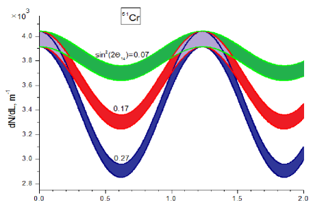
$L\rightarrow$ meters

Figure 1: Oscillation spectra with different values of $\sin{{}^{2}(2\theta_{14})}$= 0.07, 0.17 and 0.27 on the corresponding colored curves with the statistical corridor of 1$\sigma$. The values on the y-axis are obtained for 55 days of measurement with a ⁵¹Cr source and an Ar target under a pressure of 10 bar. In all cases we have included distances up to $1.5\times L_{42}$. The pattern is repeated two times up to the radius of the sphere $R_{0}$= 4 m.

The results presented in Fig. 1 did not take into consideration the electron energy threshold of 0.1 keV, which is too small in comparison with the neutrino energy and the average electron recoil energy. We neglected also the Solar background of 2 counts per day derived from the measured Borexino results Arpesella et al. (2008), BOR . It is obvious that STPC should be installed in an underground laboratory surrounded with appropriate shield against rock radioactivity.

In conclusion, we propose to use the oscillometry method for direct observation of the fourth neutrino appearance. The calculations and analysis shows that neutrino oscillometry with the gaseous STPC is a powerful tool for identification of a new neutrino in the neutrino-electron scattering. Since the expected mass-difference for this neutrino is rather high, the corresponding oscillation length is going to be sufficiently small for 1 MeV neutrino energy so that it can be fitted into the dimensions of a spherical detector with the radius of a few meters. The neutrino oscillometry can be implemented in this detector with the use of the intense monochromatic neutrino sources which can be placed at the origin of sphere and suitably shielded. The gaseous STPC with the Micromegas detection has a big advantage in the 4$\pi$-geometry and in very good position resolution (better than 0.1 m) with a very low energetic threshold ($\approx$ 100 eV). The most promising candidates for oscillometry have been considered. The sensitivity for one of them, e.g. ⁵¹Cr, to the mixing angle $\theta_{14}$ is estimated as $\sin{{}^{2}(2\theta_{14})}$ = 0.05 with the 99% of confidence, which can be reached after two months of data handling. This value can be pushed further down by using renewable sources. The observation of the oscillometry curve suggested in this work will be a definite manifestation of the existence of a new type of neutrino, like the one recently proposed by the analysis of the low energy neutrino anomaly.

A help of D. Nesterenko in preparation of this manuscript is very much acknowledged.

References

- (1) G. Mention, M. Fechner, Th. Lasserre, Th. A. Mueller, D. Lhuillier, M. Cribier, A. Letourneau, The Ractor Neutrino Anomaly, arXiv:1101.2755 [hep-ex] (2011).
- Giunti and Laveder (2010) C. Giunti and M. Laveder, Phys. Rev. D 32, 053005 (2010).
- Giomataris and Vergados (2006) Y. Giomataris and J. Vergados, Phys. Lett. B 634, 23 (2006), ; hep-ex/0503029.
- Vergados and Novikov (2010) J. Vergados and Y. Novikov, Nucl. Phys. B 839, 1 (2010), arXiv:1006.3862[hep-ph].
- (5) J.D. Vergados, Y. Giomataris and Yu. N. Novikov, Probing the fourth neutrino existence by neutral current oscillometry in the spherical gaseous TPC, arXiv:1103.5307 (hep-ph).
- (6) J.D. Vergados, Y. Giomataris and Yu. N. Novikov, Proceedings of PASCOS10 (Valencia spain) and Neutrino 2010 (Athens Greece), arXiv:1010.4388 [hep-ph].
- Blaum et al. (2010) K. Blaum, Y. Novikov, and G. Werth, Contemp. Phys. 51, 149 (2010), [arXiv:0909.1095](physics.atom-ph).
- Larkins (1977) F. Larkins, At. Data and Nucl. Data Tables 20, 311 (1977).
- Audi et al. (2003) G. Audi et al., Nucl. Phys. A 729, 3 (2003).
- (10) Nuclear Data Sheets, The US National Data Center, http://www.nndc.bnl.gov.
- S.Andriamonje et al. (2010) S.Andriamonje et al., JINST 5, P02001 (2010).
- Cebrian et al. (2010) C. Cebrian et al., JCAP 1010, 010 (2010).
- Giomataris et al. (1996) Y. Giomataris et al., Nucl. Instr. and Meth. A 376, 29 (1996).
- Giomataris et al. (2008) I. Giomataris et al., JINST 3, P09007 (2008), arXiv:0807.2802 (physics.ins-det).
- Arpesella et al. (2008) C. Arpesella et al., Phys. Rev. Lett. 101, 091302 (2008).
- (16) M. Pallavicini, for the Borexino Collaboration, Proceedings of the RICAP 2009 workshop; arXiv:0910.3367 [hep-ex].