All-loop calculation of the Reggeon field theory amplitudes via stochastic model

Abstract

The evolution equations for Green functions of the Reggeon Field Theory (RFT) are equivalent to those of the inclusive distributions for the reaction-diffusion system of classical particles. We use this equivalence to obtain numerically Green functions and amplitudes of the RFT with all loop contributions included. The numerical realization of the approach is described and some important applications including total and elastic proton–proton cross sections are studied. It is shown that the loop diagram contribution is essential but can be imitated in the eikonal cross section description by changing the Pomeron intercept. A role of the quartic Pomeron coupling which is an inherent part of the stochastic model is shown to be negligible for available energies.

1 Introduction.

The Reggeon Field Theory (RFT) [1] is successfully used up to nowadays for describing the soft part of the strong interaction dynamics at high energies. It is based on the very general principles which should obey $s$-channel amplitudes such as analiticity, crossing and $t$-channel unitarity. Particular field theories like QCD should obey the same principles. The Regge-like behavior was observed in QCD and some of the RFT components which are not deducible from the first principles like the Pomeron intercept were obtained within certain approximations. These approximations of the QCD however are questionable to apply to the processes which do not involve high momentum transfer. Moreover, it is rather complicated to fulfil the reqirements of full many-particle $t$-channel unitarity which is very important for high-energy dynamics. Due to the generality and phenomenological success of the RFT in many aspects it can be viewed as complementary to the QCD and should be treated on the equal grounds with the QCD-induced models.

For the description of the experimental data in the reggeon approach one usually uses the simplest reggeon diagrams corresponding to the pomeron pole and a set of nonenhanced regge-cut graphs providing $s$-channel unitarity. However for the case of the supercritical pomeron (with the intercept larger than one) the interaction between pomerons may be essential and can become especially important at the LHC energies so the contribution of loop reggeon diagrams should be estimated. In this paper we present such estimates for the RFT with triple and quartic pomeron vertices using the mathematical equivalence of this theory to dynamics of stochastic system of classical particles [2].

The Lagrangian density of the Reggeon Field Theory is formulated by using the non-relativistic Pomeron field $\phi(y,{\bf b})$

$$\mathcal{L}=\frac{1}{2}\phi^{\dagger}(\overleftarrow{\partial_{y}}-\overrightarrow{\partial_{y}})\phi-\alpha^{\prime}(\nabla_{\bf b}\phi^{\dagger})(\nabla_{\bf b}\phi)+\Delta\phi^{\dagger}\phi+\mathcal{L}_{int}~{},$$ (1)

where the rapidity $y$ plays a role of time, ${\bf b}$ represents position in the impact parameter plane, parameters $\alpha^{\prime}$ and $\Delta$ describe the linear Pomeron trajectory, $\alpha_{P}(t)=(1+\Delta)+\alpha^{\prime}t$, and $L_{int}$ contains the interaction terms. The usual choice for the interaction terms is the option when it generates only triple Pomeron vertices, however terms of higher order in $\phi$ and $\phi^{\dagger}$ can also enter.

It was shown in [2] and discussed in the subsequent papers [3, 4] that the classical stochastic system of particles (called “partons” for brevity) which undergo diffusion in 2-dimensional space and interact in a specific way (the particles can split, die, fuse or annihilate in pairs) allows a field-theoretical realization corresponding to the RFT Lagrangian (1) with

$$\mathcal{L}_{int}=i\,r_{{\scriptscriptstyle 3P}}\phi^{\dagger}\phi(\phi^{\dagger}+\phi)+\chi{\phi^{\dagger}}^{2}\phi^{2}+j_{0}\phi^{\dagger}+j_{Y}\phi~{}.$$ (2)

The interaction includes both triple (nonhermitian) and quartic terms, the source term $j_{0}(0,{\bf b})$ gives the initial condition for the $y$-evolution (“parton” distribution in the projectile) and the term $j_{Y}(Y,{\bf b})$ describes the partonic structure of the target and is necessary for calculating the scattering amplitude at total rapidity $Y$. The values of the Reggeon couplings in (2) are connected with the rate parameters of the stochastic model. Equality of couplings $r_{{\scriptscriptstyle 3P}}$ for both triple terms in (2) imposed by Lorentz invariance requires tuning of the parameters. The multiparticle inclusive distributions of the stochastic system turn out to be identical to the Green functions of the RFT. This correspondence may be used to compute the amplitudes of that specific model of the Reggeon field theory with the account of all loops.

In this paper we present a numerical realization of the stochastic approach and give some estimates of the loop diagram contribution for the RFT in $d=0$ and $d=2$ dimensions. In the next section we recall the notations and the definitions of the stochastic approach and outline the correspondence between the parameters of the RFT and that of the stochastic approach. Section 3 is devoted to the description of the numerical method used for the computations of the amplitude. In Section 4 we analyze asymptotic behaviour of the Pomeron Green function in $d=0$ and $d=2$ dimensions for various sets of parameters. The role of the quartic Pomeron coupling is discussed. In Section 5 the correspondence between the parameters of the stochastic model and the couplings of the Reggeon field theory is established by comparing contributions of simplest diagrams. We also discuss the restrictions which one must impose on the numerical algorithm to reproduce the contribution of the limited sets of the Reggeon diagrams which enter in the (quasi)eikonal approximation. Then the calculated contribution to proton-proton cross sections of the full set of the Reggeon diagrams is compared to the standard calculations in the quasieikonal approximation and the role of the Pomeron interactions is estimated. The effective change of the Pomeron intercept due to account of these interactions is found. Concluding remarks are presented in the last section.

2 The stochastic model

Here we briefly describe the stochastic model of the RFT (also known as reaction-diffusion approach) as it is formulated in [3]. We follow the evolution of the system of classic particles, “partons”, which interact in a certain way. The partons are allowed to move randomly in the transverse plane, and this diffusive motion is described by a diffusion coefficient $D$. The particles can split, $A\rightarrow A+A$, with a splitting probability per unit time $\lambda$, or die, $A\rightarrow\emptyset$, with a death probability $m_{1}$. When two partons are brought within the reaction range due to the diffusion, they can pairwise fuse, $A+A\rightarrow A$, or annihilate, $A+A\rightarrow\emptyset$. To describe the rate of these processes we use dimensional fusion and annihilation constants, $\sigma_{\nu}$ and $\sigma_{m_{2}}$:

$$\sigma_{\nu}\equiv\int d^{2}b\,p_{\nu}(b)~{},\quad\sigma_{m_{2}}\equiv\int d^{2}b\,p_{m_{2}}(b)~{}.$$ (3)

The dimension of $\sigma_{m_{2}}$ and $\sigma_{\nu}$ thus is length squared. The characteristic scale, that is the effective interaction distance, is determined by the functions $p_{\nu}(b)$ and $p_{m_{2}}(b)$. It is assumed to be small compared to the characteristic scale of the problem (e.g. proton radius).

Throughout the evolution the system of partons is described by a set of symmetrized probability densities $\rho_{\scriptscriptstyle N}(y;{\bf b}_{1},\ldots,{\bf b}_{N})$ of finding exactly $N$ partons at evolution time $y$ at positions $\{{\bf b}_{1},\ldots,{\bf b}_{N}\}$ in the transverse plane. For brevity we use the notation ${\cal B}_{N}$ for the set $\{{\bf b}_{1},\ldots,{\bf b}_{N}\}$ and $d{\cal B}_{N}$ for $d{\bf b}_{1}\ldots d{\bf b}_{N}$. The probability densities are normalized according to

$$\frac{1}{N!}\int d{\cal B}_{\scriptscriptstyle N}\rho_{\scriptscriptstyle N}(y;{\cal B}_{\scriptscriptstyle N})=p_{\scriptscriptstyle N}(y),$$ (4)

where $p_{N}(y)$ is the probability of having exactly $N$ partons at the evolution time $y$, $\sum p_{N}(y)=1$.

The important quantities which have a direct analog in the Reggeon field theory are the inclusive $s$-parton distributions, which correspond to observing $s$ partons at positions ${\cal Z}_{s}=\{{\bf z}_{1},\ldots,{\bf z}_{s}\}$ and integrating out all the rest. They are defined as

$$f_{s}(y;{\cal Z}_{s})=\sum_{N}\cfrac{1}{(N-s)!}\int\!d{\cal B}_{N}\;\rho_{\scriptscriptstyle N}(y;{\cal B}_{N})\prod_{i=1}^{s}\delta({\bf z}_{i}-{\bf b}_{i}).$$ (5)

Due to the symmetry properties of $\rho_{N}(y;{\cal B}_{N})$ the inclusive distributions $f_{s}(y;{\cal Z}_{s})$ are also symmetric functions of their variables. As follows from the normalization of the $\rho_{\scriptscriptstyle N}$, the inclusive distributions are normalized to the factorial moments $\mu_{s}$ of the distribution $p_{\scriptscriptstyle N}(y)$:

$$\int d{\cal Z}_{s}f_{s}(y;{\cal Z}_{s})=\sum\frac{N!}{(N-s)!}\,p_{N}(y)\equiv\mu_{s}(y).$$ (6)

As it is pointed out in [3] the evolution equations in time $y$ for the inclusive distributions $f_{s}(y;{\cal Z}_{s})$

$$\frac{d}{dy}f_{s}(y;{\cal Z}_{s})=\,D\,{\nabla}_{s}^{2}f_{s}(y;{\cal Z}_{s})\!+\!(\lambda-m_{1})sf_{s}(y;{\cal Z}_{s})+\\ \phantom{\frac{d}{dy}}\!+\!\lambda\!\sum_{k,l=1}^{s\geqslant 2}f_{s-1}(y;{\cal Z}_{s}^{(l)})\delta({\bf z}_{k}-{\bf z}_{l})\!-\!\nu\!\sum_{k,l=1}^{s\geqslant 2}f_{s}(y;{\cal Z}_{s})\delta({\bf z}_{k}-{\bf z}_{l})-\\ \phantom{\frac{d}{dy}}\!-\!(2m_{2}+\nu)\!\sum_{k=1}^{s}f_{s+1}(y;{\cal Z}_{s}^{(k)},{\bf z}_{k},{\bf z}_{k})~{},\qquad(s=1,2,\ldots)$$ (7)

exactly reproduce the evolution equations in rapidity for the Green functions of the RFT with the interaction term (2). This means that the inclusive distributions themselves are proportional to the Green functions of the RFT in convolution with the particle–$m$-Pomeron vertices of the RFT $\mathcal{N}_{m}({\cal X}_{m})$:

$$f_{s}(y;{\cal Z}_{s})\propto\sum_{m}\int d{\cal X}_{m}\,\mathcal{N}_{m}({\cal X}_{m})G_{mn}(0;{\cal X}_{m}|y;{\cal Z}_{n})~{}.$$ (8)

where the Green functions $G_{mn}(0;{\cal X}_{m}|y;{\cal Z}_{n})$ describe the transition of $m$ Pomerons at rapidity $y=0$ into $n$ Pomerons at rapidity $y$. The proportionality factor takes into account the dimension of the inclusive distributions and should be specified at calculating Regge amplitudes (see below). The vertices $\mathcal{N}_{m}({\cal X}_{m})$ determine the initial distribution of partons in number and transverse positions at zero time $y=0$ which are used as a starting point for the evolution of $f_{s}$. We will attend to this point in section 5.

The amplitude of the RFT as a function of the total rapidity $Y$ and impact parameter ${\bf b}$ is expressed in terms of the set of the inclusive partonic distributions $f_{s}(y,{\cal Z}_{s})$ for the projectile $A$ and $\tilde{f_{s}}(Y-y,\tilde{\cal Z}_{s})$ for the target $\tilde{A}$ taken at arbitrary intermediate rapidity $y$ through the procedure of linkage:

$$T(Y)=\langle A|T|\tilde{A}\rangle=\sum_{s=1}^{\infty}\frac{(-1)^{s-1}}{s!}\int d{\cal Z}_{s}d\tilde{\cal Z}_{s}f_{s}(y;{\cal Z}_{s})\tilde{f}_{s}(Y-y;\tilde{\cal Z}_{s})\prod_{i=1}^{s}g({\bf z}_{i}-\tilde{\bf z}_{i}-{\bf b}).$$ (9)

This procedure realizes a linkage of partons (Pomerons) of the target and the projectile through a convolution with the linking functions $g(\ldots)$. These functions are narrow functions of the $\delta$-function type normalized to some parton size $\epsilon=\pi a^{2}$. They will be specified in section 3.

The formula (9) links two partonic cascades coming from the target and the projectile at the rapidity value $y$. It was proved in [3] that, provided the scales of the functions $g(b)$, $p_{\nu}(b)$ and $p_{m_{2}}(b)$ are small, the convolution (9) depends only on the overall rapidity/evolution time $Y$ but not on the position of the linking point $y$ if a certain condition on the model parameters is satisfied. Namely,

$$\lambda\int g(b)db=\int p_{m_{2}}(b)db+\frac{1}{2}\int p_{\nu}{b}db~{},$$ (10)

or,

$$\lambda\epsilon=\sigma_{m_{2}}+\frac{1}{2}\sigma_{\nu}~{}.$$

This condition in fact corresponds to the equality of the Pomeron fusion and splitting vertex.

The relation between the Reggeon field theory parameters and the ones of the stochastic model is given in table 1.

Table 1: Relation between the parameters of the RFT and those of the stochastic approach.

RFT	stochastic model
Rapidity $y$	Evolution time $y$
Slope $\alpha^{\prime}$	Diffusion coefficient $D$
$\Delta=\alpha(0)-1$	$\lambda-m_{1}$
Splitting vertex $r_{{\scriptscriptstyle 3P}}$	$\lambda\sqrt{\epsilon}$
Fusion vertex $r_{{\scriptscriptstyle 3P}}$	$(\sigma_{m_{2}}+\tfrac{1}{2}\sigma_{\nu})/\sqrt{\epsilon}$
Quartic coupling $\chi$	$\tfrac{1}{2}(\sigma_{m_{2}}+\sigma_{\nu})$

Since the inclusive distributions (5) are in direct correspondence with the exact Green functions of the RFT with the account of all loops (the model characteristic scale of $p_{\nu}$ and $p_{m_{2}}$ plays a role of the cutoff for the RFT Green functions), the equation (9) can be used for obtaining the exact numerical answer for the RFT scattering amplitude.

3 Numerical method.

The inclusive distributions $f_{s}$ and $\tilde{f}_{s}$ which enter (9) are defined by the evolution of the partonic subsystems with a certain initial distribution of partons in their number and transverse positions. Basically one may assume a straightforward way of calculating the interaction amplitude according to (9) by making a Monte-Carlo average over the initial conditions and computing $f_{s}$ and $\tilde{f}_{s}$ explicitly. This method, however, seems to be numerically unaffordable. For example, besides the evolution of partonic system and computing the distributions $f_{s}$ on some grid which one has to introduce, it is necessary to perform symmetrization of the $f_{s}$’s which (provided the grid has fairly small cells) is extremely time consuming, or, alternatively, increase the number of Monte-Carlo simulations in the same proportion. The corresponding number of operations can be estimated as $M!/(M-s)!$, which is the number of choices of $s$ out of $M$ points of the grid together with number of transpositions.

Let’s rewrite (9) explicitly indicating the averaging over the initial distribution of partons:

$$T(Y)=\sum_{s=1}^{\infty}\frac{(-1)^{s-1}}{s!}\sum_{n,\tilde{n}}\int d{\cal B}_{n}d\widetilde{\cal B}_{\tilde{n}}P({\cal B}_{n})\widetilde{P}(\widetilde{\cal B}_{\tilde{n}})\\ \int d{\cal Z}_{s}d\widetilde{\cal Z}_{s}f_{s}(y;{\cal B}_{n}|{\cal Z}_{s})\tilde{f}_{s}(Y-y;\widetilde{\cal B}_{\tilde{n}}|\widetilde{\cal Z}_{s})\prod_{i}g({\bf z}_{i}-\tilde{\bf z}_{i}-{\bf b})$$ (11)

Here $f_{s}(y;{\cal B}_{n}|{\cal Z}_{s})$ and $\tilde{f}_{s}(Y-y;\widetilde{\cal B}_{\tilde{n}}|\widetilde{\cal Z}_{s})$ stand for the $s$-parton inclusive distributions obtained upon the evolution of the initial sets of projectile-associated partons at positions ${\cal B}_{n}$ and of target-associated partons at $\widetilde{\cal B}_{\tilde{n}}$. The straightforward way of calculations described above consists in averaging over the sets ${\cal B}_{n}$ and $\widetilde{\cal B}_{\tilde{n}}$ prior to the integration over ${\cal Z}_{s}$ and $\widetilde{\cal Z}_{s}$.

Another way of calculations can be realized making averaging over $\{n,B_{n}\}$ and $\{\tilde{n},\widetilde{B}_{\tilde{n}}\}$ after the convolution in ${\cal Z}_{s}$ and $\tilde{Z}_{s}$. In other words, the Monte-Carlo averaging is done for the amplitude computed on the “samples”, particular realizations of the probability distributions which correspond to the set of inclusive distributions $f_{s}$ and $\tilde{f}_{s}$. Each sample is generated by evolving a set of partons in rapidity starting from the random number and initial positions of partons generated according to the distributions $P(n,{\cal B}_{n})$ and $\widetilde{P}(\tilde{n},\widetilde{\cal B}_{\tilde{n}})$.

A set of $N$ partons with fixed coordinates $\widehat{\cal X}_{N}=\{\hat{\bf x}_{1},\ldots,\hat{\bf x}_{N}\}$ in the transverse plane corresponds to the following set of the $s$-parton inclusive distribution functions $f_{s}(Z_{s})$ ($s=1\ldots N$):

$$f_{s}({\cal Z}_{s})=\sum_{\{\hat{\bf x}_{i_{1}},..,\hat{\bf x}_{i_{s}}\}\in\hat{\cal X}_{N}}\delta({\bf z}_{1}-\hat{\bf x}_{i_{1}})\ldots\delta({\bf z}_{s}-\hat{\bf x}_{i_{s}}).$$ (12)

The sum goes over all the ordered subsets of $s$ variables out of $N$ which ensures the normalization of $f_{s}$ and its symmetry properties. The same is for $\tilde{f}_{s}(\widetilde{\cal Z}_{s})$ where the parton coordinates $\hat{y}_{i}\in{\cal Y}_{\tilde{N}}$. After substituting (12) the sample amplitude (cf. with (11)) reads:

$$T_{\rm sample}=\sum_{s=1}^{N_{min}}\frac{(-1)^{s-1}}{s!}\sum_{\begin{subarray}{c}i_{1},\ldots,i_{s}=1\\ i_{m}\neq i_{l}\end{subarray}}^{N}\ \sum_{\begin{subarray}{c}j_{1},\ldots,j_{s}=1\\ j_{m}\neq j_{l}\end{subarray}}^{\tilde{N}}g(\hat{\bf x}_{i_{1}}-\hat{\bf y}_{j_{1}})\ldots g(\hat{\bf x}_{i_{s}}-\hat{\bf y}_{j_{s}}).$$ (13)

Here $N$ and $\tilde{N}$ are the numbers of partons in the samples which come from the evolution of the projectile- and the target-associated sets of partons and $N_{min}=\min(N,\tilde{N})$ is the minimal number of partons in these two samples.

The values

$$g_{ij}\equiv g(\hat{\bf x}_{i}-\hat{\bf y}_{j})$$ (14)

computed on the samples of partons form a matrix which can be looked upon as the adjacency matrix of the bipartite graph with weights $g_{ij}$.

For a given $s$ in the sum (13) there are $s!$ identical terms which correspond to permutations of the pairs $\{{\bf x}_{i},{\bf y}_{j}\}$. This is since the summation in (13) is goes not only over the subsets $\{i_{1},\ldots,i_{s}\}\in\{1,\ldots,N\}$ and $\{j_{1},\ldots,j_{s}\}\in\{1,\ldots,\tilde{N}\}$ but also over the permutations within these subsets due to symmetrized form of $f_{s}({\cal Z}_{s})$. Taking this into account we arrive at the expression

$$T_{\rm sample}=\sum_{s=1}^{N_{min}}(-1)^{s-1}\sum_{i_{1}<i_{2}\ldots<i_{s}}\sum_{j_{1},\ldots,j_{s}}g_{i_{1}j_{1}}\ldots g_{i_{s}j_{s}}.$$ (15)

It means that for each term of the sum with fixed $s$ one has to take all possible products of $s$ elements of the matrix $G=\|g_{ik}\|$ so that the elements from the same line or column would not enter same product. The products with the odd number of multipliers enter with $+1$, the ones with the even – with $-1$. Speaking in terms of mathematical definitions, this is a sum of the permanents of all the square submatrices of the matrix $G=\{g_{ij}\}$ with alternating sign. The submatrices are obtained from the initial matrix $G$ by removing the relevant number of lines and columns.

The permanent of a matrix (see e.g. [7]) has a definition analogous to that of the determinant, but without the alternation of the sign in the sum:

$$\mbox{Per}\{A\}=\sum_{\pi\in S_{n}}\prod_{i=1}^{n}a_{i,\pi_{i}}$$ (16)

Despite its similarity with the determinant, the permanent is quite an inconvenient construction for a numerical computation. The fastest known algorithm is given by the Ryser formula:

$$\mbox{Per}(A)=(-1)^{n}\sum_{S\subseteq\{1,\dots,n\}}(-1)^{|S|}\prod_{i=1}^{n}\sum_{j\in S}a_{ij},$$ (17)

where summation goes over all the subsets $S$ of $\{1\ldots n\}$ and $|S|$ denotes the number of elements in the subset. The number of operations for computing according to this formula is around $O(2^{n}n)$. This is much less than $O(n!)$ needed for the straightforward computation according to (16), however still incomparable with $O(n^{2})$ operations needed for computing the determinant.

One can easily generalize Ryser formula for the case of the amplitude $T_{\mathrm{sample}}$ in (15):

$$T_{\mathrm{sample}}=\sum_{s_{1}\subseteq\{1,\dots,N\}}\sum_{\begin{subarray}{c}s_{2}\subseteq\{1,\dots,\tilde{N}\},\\ |s_{2}|<|s_{1}|\end{subarray}}(-1)^{|s_{2}|-1}{\rm C}_{\tilde{N}-|s_{2}|}^{|s_{1}|-|s_{2}|}\prod_{i\in s_{1}}\left(\sum_{j\in s_{2}}g_{ij}\right)~{}.$$ (18)

The estimated number of operations here is around $O(n4^{n})$ for a sample, which is much less than the number of operations required for symmetrization of the full set of inclusive distributions $f_{s}({\cal Z}_{s})$ on the grid in the straightforward way of the amplitude calculation.

Calculations based on the Monte-Carlo averaging of (18) allow to to set an arbitrary rapidity for the linkage point since the amplitude $T$ depends only on the overall rapidity, that is the sum of the evolution times of two samples, as proven in [3]. The freedom in the choice of the linkage point can be quite convenient for calculating the amplitude at large rapidities when the Pomeron intercept exceeds unity. In this case the number of partons in the set grows exponentially with the evolution time and at some point the Monte-Carlo evolution of the set can become very numerically expensive. So choosing the linkage point e.g. as a half of the overall rapidity can in principle compensate the difficulties connected with the computing of the permanents. Besides this, (18) also serves as an expansion in the number of Pomeron exchanges $|s_{1}|$ between the upper and lower blocks of the amplitude at the rapidity of the linkage point.

If the application which we are using the stochastic approach for do not involve this expansion and the overall rapidity is not too large, a much less numerically expensive method can be used. Taking advantage of the independence of the amplitude (9) on the linkage point we use the fact that for zero evolution time the inclusive distributions $\tilde{f}_{s}(y=0,{\cal Z}_{s})$ are proportional to the particle–$m$Pomerons vertices (cf. (8)) and hence are known. Substituting (12) into the (9) together with the known functions $\tilde{f}_{s}(y=0,{\cal Z}_{s})$ and as before taking into account the symmetry properties of $f_{s}(Y,{\cal Z}_{s})$ in (12) we have:

$$T_{\rm sample}({\bf b})=\sum_{s=1}^{N}(-1)^{s-1}\tilde{\mu}_{s}\epsilon^{s}\sum_{i_{1}<i_{2}\ldots<i_{s}}\tilde{p}(\hat{\bf x}_{i_{1}}-{\bf b},\ldots,\hat{\bf x}_{i_{s}}-{\bf b}).$$ (19)

Here $\tilde{\mu}_{s}$ denotes the factorial moments of the distribution which corresponds to the set $\tilde{f}_{s}(y=0,{\cal Z}_{s})$ and $\tilde{p}_{s}$ stands for its coordinate dependent part normalized to unity. In writing (19) we also assumed that the functions $g({\bf x})$ are narrow and replaced them by $\epsilon\delta({\bf x})$. In case of no correlations in the vertex which for example is the case for the eikonal vertices $\tilde{p}_{s}({\cal Z}_{s})=\prod p_{\tilde{A}}({\bf z}_{i})$ and (19) reads

$$T_{\rm sample}({\bf b})=\sum_{s=1}^{N}(-1)^{s-1}\tilde{\mu}_{s}\epsilon^{s}\sum_{i_{1}<i_{2}\ldots<i_{s}}p_{\tilde{A}}(\hat{\bf x}_{i_{1}}-{\bf b})\ldots p_{\tilde{A}}(\hat{\bf x}_{i_{s}}-{\bf b}).$$ (20)

The amplitude is obtained as the Monte-Carlo average of (19) or (20) over the sets of partons.

For the numerical calculations one must also fix the form of the distributions $p_{m_{2}}(b)$ and $p_{\nu}(b)$ together with making a specific choice for the functions $g(b)$ in the convolution (9). We take these distributions in the following form:

$$p_{m_{2}}({\bf b}) = m_{2}\;\uptheta(a_{m_{2}}-|{\bf b}|);$$ (21)

$$p_{\nu}({\bf b}) = \nu\;\uptheta(a_{\nu}-|{\bf b}|);$$ (22)

$$g({\bf b}) = k\;\uptheta(a-|{\bf b}|);$$ (23)

where we have introduced explicitly the interaction and convolution scales; the constants $\nu$ and $m_{2}$ play a role of fusion and annihilation probabilities for a pair of partons per unit time provided they are close enough in the transverse plane; $k$ is some appropriate numerical factor . The boost invariance condition (10) in these notations reads:

$$\lambda k\pi a^{2}=m_{2}\pi a_{m_{2}}^{2}+\tfrac{\nu}{2}\pi a_{\nu}^{2}$$ (24)

while triple and quartic coupling constants are

$$\begin{array}[]{l}r_{3P}=\lambda\sqrt{\pi k}a=\sqrt{\tfrac{\pi}{k}}(m_{2}a_{m_{2}}^{2}+\tfrac{1}{2}\nu a_{\nu}^{2})/{a};\\ \chi=\tfrac{\pi}{2}(m_{2}a_{m_{2}}^{2}+\nu a_{\nu}^{2}).\end{array}$$ (25)

For a given value of the triple coupling $r_{3P}$ by taking a higher value for the parameter $k$ one can release the scale $a$ and set it small enough compared to the characteristic scale of the problem, which is, as mentioned, the condition of applicability of the stochastic approach. Though three radii can in principle differ, in our numerical calculations for clarity we take all three the same $a_{m_{2}}=a_{\nu}=a$. To reduce the number of free parameters in the model we also choose $k=1$. The boost invariance condition for our choice takes the most simple form:

$$\lambda=m_{2}+\nu/2~{}.$$ (26)

The elastic amplitude is computed as a Monte-Carlo average of the expressions (13) or (19) over the sets of partons which underwent stochastic evolution over the given time (rapidity) interval. The way of preparing these sets is straightforward. First, the number of partons and their position in the transverse plane are generated acccording to the distribution defined by the particle–$m$-Pomeron vertices. After this, based on the position of partons in the transverse plane we define a probabilities $\gamma_{i}$ of splitting, death, fusion and annihillation of partons per unit time provided they preserve their positions. The survival probability (probability of having no change in the number of partons) as a function of time $y$ in this case is a simple exponential $p(y)=\exp(-\sum\gamma_{i}y)$.

We generate time interval $\delta y$ before the change in the parton number according to the distribution $p(y)$. If the time interval does not exceed $y_{0}=0.1a/\sqrt{D}$ (10% of the characteristic diffusion timescale) we define the type of the changing number event (toss it according to the total splitting, death, annihillation and fusion probabilities) and a candidate parton or a parton pair. Then we randomly change the positions of all the partons in the set according to the diffusion law with the time $\delta y$, do the necessary change in the number of partons and recalculate the number change probabilities $\gamma_{i}$ with the new parton number and the partons new coordinates.

If the time interval $\delta y$ exceeds $y_{0}$ we change the positions of partons in the set according to the diffusion law with the time $y_{0}$ and recalculate the probabilities $\gamma_{i}$.

The steps are repeated until we reach the desired overall evolution time.

4 The Pomeron propagator

Now it is straightforward to attend to the numerical studies of the RFT. As a first example we compare exact numerical results for the Pomeron propagator in zero-dimensional RFT and RFT with the account of diffusion. The zero-dimensional case has been studied before both analytically in a series of works starting from [8] and numerically ( e.g. [9]) for zero value of the quartic coupling. The most important result was the decrease of the two-point Green function or the Pomeron propagator (describing transition of one Pomeron into one Pomeron) with rapidity although the perturbative propagator has an exponential growth. It has also been reported in [4] that in the zero-dimensional theory with the $2\to 2$ coupling a constant asymptotic behaviour of the propagator is possible for some special choice of the quartic coupling, namely $\chi=r_{3P}^{2}/\Delta$ in our notations.

In terms of the stochastic model the propagator is the single particle inclusive distribution $f_{1}(y,{\bf b})$ for the state which have evolved out of a single parton at $y=0$ (see (8)). The transition to zero-dimensional case is made in our numerical approach by setting the diffusion coefficient equal to zero. Within our calculation scheme we investigate the role of the quartic Pomeron coupling in the asymptotic behaviour of the propagator or amplitude in both zero and two transverse dimensions Reggeon field theory.

We start with the zero dimensions case. Our aim is to illustrate the role of the enhanced diagrams simply comparing the simple pole contribution to the propagator with the result of the full numerical computation.

Here the propagator as a function of rapidity is simply the average number of partons as a function of the evolution time. The evolution starts with a single parton. In fig.1 we present calculations for different sets of the parameters $\lambda$, $\nu$, $m_{1}$, $m_{2}$ (see table2). The values of the parameters correspond to the same value of the intercept $\Delta=\lambda-m_{1}=0.1$, satisfy the Lorenz invariance condition in zero dimensions $\lambda=m_{2}+\nu/2$ (cf. eq.(66) of [3]) and differ by values of the couplings $r_{{\scriptscriptstyle 3P}}=\lambda$ and $\chi=(m_{2}+\nu)/2$ only.

Table 2: Parameters of the model and the RFT couplings

Set $\lambda$ $\nu$ $m_{1}$ $m_{2}$ $\Delta$ $r_{{\scriptscriptstyle 3P}}$ $\chi$ 1 0.1 0.2 0 0 0.1 0.1 0.1 2 0.1 0.1 0 0.05 0.1 0.1 0.075 3 0.1 0 0 0.1 0.1 0.1 0.05 4 0.15 0.3 0.05 0 0.1 0.15 0.15 5 0.15 0 0.05 0.15 0.1 0.15 0.075

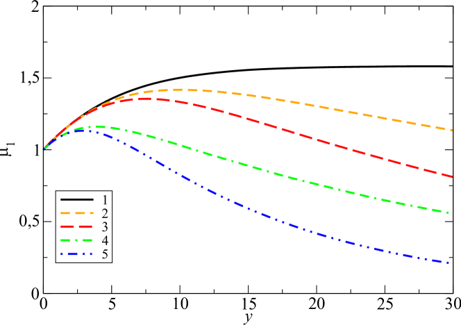
Figure 1: The full Pomeron propagator in zero dimensions as a function of rapidity. The stochastic model parameters corresponding to the sets 1–5 are in the text.

As one can see from fig. 1, the asymptotic behaviour of the propagator for zero-dimensional theory strongly depends on the relative values of $m_{2}$ and $\nu$ or, in terms of the RFT on the relation between the intercept and the couplings. The only possibility to have constant asymptotic behaviour distinct from zero within the stochastic approach is to put $m_{2}=m_{1}=0$ as in the set 1. This corresponds to equal triple and quartic coupling with $\Delta=\lambda$ (where $\Delta+1$ is the Pomeron intercept) within zero dimensional RFT which evidently satisfies the condition necessary for the constant propagator asymptotic behaviour outlined in [4]. The constant asymptotical value corresponds to the eq. (27) of [3] $\mu_{1}(\infty)=e/(e-1)\approx 1.582$. The same result is obtained by explicitly solving numerically the differential equation (eq. (6) of [3]) for generating function of the probability distribution.

Let us emphasize that all parameters of the stochastic model should be positive. Another strong restriction is given by the Lorentz invariance condition which excludes some increasing regimes of the stochastic model.

For the two dimensional case we take the same values of the stochastic model parameters as for the zero-dimensional one. Additionally we introduce the partonic interaction distance $a=0.05$ fm and the diffusion coefficient $\alpha^{\prime}=0.01$ fm${}^{2}=0.26$ GeV^-2. The Pomeron propagator now is a function of both rapidity and impact parameter. The pole contribution or the bare propagator reads

$$G(y,b)=\frac{1}{4\pi\alpha^{\prime}y}\exp\left(\Delta y-\frac{b^{2}}{4\alpha^{\prime}y}\right).$$ (27)

It goes to delta function when the rapidity $y$ goes to zero and its value at $b=0$ is growing with rapidity as $\sim e^{\Delta y}/y$.

In figure 2 we show the calculation of the full propagator as a function of impact parameter in comparison with the bare one for different rapidities. The calculations show a negligible difference between sets of parameters which correspond to the same value of the triple coupling $r_{{\scriptscriptstyle 3P}}$ and differ only by the value of the quartic coupling $\chi$ ($\{1,2,3\}$ and $\{4,5\}$). This supports the statement of [10] that presence of a finite number of higher than triple order terms in the RFT interaction Lagrangian may be ignored.

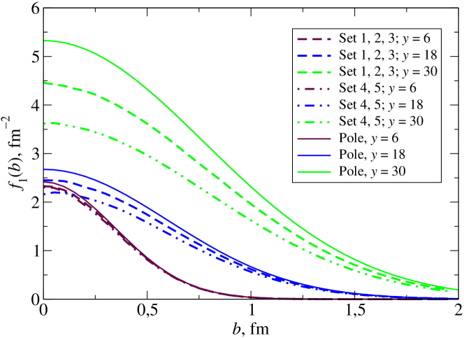
Figure 2: The full Pomeron propagator as a function of impact parameter for different values of rapidity $y$ in comparison with the perturbative one.

For making comparison with zero-dimensional case we take the value of the propagator at $b=0$ multiplied by $\epsilon=\pi a^{2}$ which in terms of the stochastic model is the average number of partons with position within that area and on the other hand is the amplitude for a single-Pomeron exchange. One may expect saturation in this quantity at sufficiently high rapidities even in presence of diffusion, since, naively speaking, at low densities parton splitting will prevail and at high densities fusion and annihilation will increase resulting in saturation eventually. However, as one can see from fig. 3 the saturation is not reached within the range of rapidity achievable by the numerical calculation, unlike the case of zero transverse dimensions which is equivalent to zero slope. This is a consequence of the fact that the value of the slope which we used and which is close to the value dictated by the fits to the experimental data (e.g [14]) is in fact quite large.

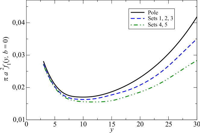
Figure 3: Full propagator scaled by $\epsilon=\pi a^{2}$ at $b=0$ as a function of rapidity in comparison with that of the bare one. The sets of constants $\lambda$, $\nu$, $m_{1}$ and $m_{2}$ are the same as used for fig. 1.

The applicability of zero dimensional approach depends on the interrelation of the parameters of the Reggeon Field Theory. Within the stochastic model the applicability condition can be formulated as follows. The number of splittings/fusions of partons must be already large for the rapidity $y_{a}$ which is required for the partons to diffuse to the distance of about the parton size.

That is, within the stochastic approach the regime similar to zero-dimensional case is realized for

$${\lambda a^{2}}\gg\alpha^{\prime}y_{a}.$$ (28)

This situation is illustrated in fig. 4 where we draw the same value as in fig. 3 for the parameter set number 1. However this time the curves correspond to different values of the slope $\alpha^{\prime}$ ranging from $0.01$ fm² to $10^{-6}$ fm² (from $0.26$ to $2.6\cdot 10^{-5}$ GeV^-2). One can easily see that the zero-dimensional regime is observed for $\alpha^{\prime}=10^{-5}$ fm² up to $y\simeq 10$ which is in agreement with the estimate (28). However, since the triple Pomeron coupling is comparatively small (and, consequently, $\lambda$ and $a$ are), it is rather the opposite limit that must be adopted for the applications and the diffusion must be fully taken into account.

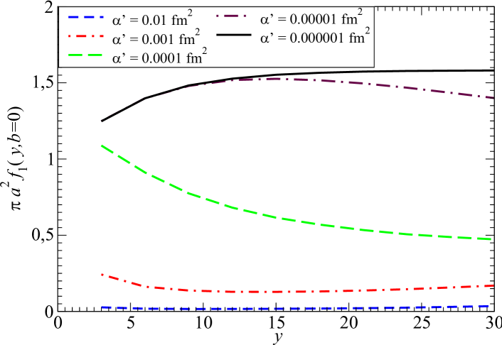
Figure 4: Full propagator scaled by $\epsilon=\pi a^{2}$ at $b=0$ for the constants $\lambda$, $\nu$, $m_{1}$ and $m_{2}$ of the set 1 and different slope $\alpha^{\prime}$ values.

To conclude, in presence of diffusion the full Pomeron propagator at a fixed distance in the transverse space for the realistic slope value dictated by fits to the experimental data is a growing function of rapidity within the reach of numerical calculations. Within this rapidity range it just expresses a slower growth than the bare one (pole contribution). This is unlike the case with the absence of diffusion where the full propagator drops at high energies or reaches constant value comparatively fast. We also note that the behaviour of the propagator at large rapidities seem to depend on the slope value in a highly nontrivial way. This points out an important role of the Pomeron slope for the set on of saturation and probable change to a subcritical behavior in the propagator. Another important distinction between the zero-dimensional and 2-dimensional theory is the role played by the quartic coupling. As one can see, the quartic coupling drastically changes the propagator asymptotic behaviour in case of zero-dimensions, while in presence of diffusion its role is negligible.

5 Total and elastic cross sections.

5.1 Normalization of the amplitudes and the couplings.

To proceed with applying the technique to the calculations of the cross sections we first fix the normalization of the amplitude. This procedure is essential for the applications as it affects definitions of the phenomenological couplings of the Pomeron to particle.

We use the elastic scattering amplitude $M(Y,{\bf q})$ normalized in such a way that

$$\sigma^{\rm tot}(Y)=2\,{\mathrm{Im}\,}M(Y,{\bf q}=0),\quad\sigma^{\rm el}=\int\frac{d^{2}q}{(2\pi)^{2}}\,|M(Y,{\bf q})|^{2}~{},$$ (29)

where $Y=\ln(s/s_{0})$, $s_{0}=1~{}~{}\mathrm{GeV}^{2}$ and ${\bf q}^{2}=-t$. The amplitude in the coordinate representation $f(Y,{\bf b})$ is defined as

$$f(Y,{\bf b})=\frac{1}{(2\pi)^{2}}\int d^{2}q\,e^{-i{\bf q}{\bf b}}M(Y,{{\bf q}})~{}.$$ (30)

With this definition of the Fourier transform, the perturbative Pomeron propagator in the coordinate representation coincides with the Green function of the diffusion equation with splitting. The cross sections are

$$\sigma^{\rm tot}(Y)=2\!\int d^{2}b\,{\mathrm{Im}\,}f(Y,{\bf b})~{},\quad\sigma^{\rm el}=\int d^{2}b\,|f(Y,{\bf b})|^{2}.$$ (31)

We neglect the small real part of the Pomeron signature factor, so in what follows the Pomeron amplitudes are considered as purely imaginary, $f(Y,{\bf b})\simeq iT(Y,{\bf b})$, $T\equiv{\mathrm{Im}\,}f$.

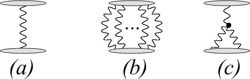
Figure 5: Reggeon graphs used for normalization of the couplings.

To establish the correspondence between the Pomeron–particle couplings and the distributions of projectile- and target-associated partons in the stochastic approach we use the contribution of single Pomeron exchange to the total cross section (fig.5a). In the standard Regge parametrization the Regge-pole contribution has the form

$$T_{\scriptstyle P}(Y,q^{2})=\beta_{A\phantom{\widetilde{A}\!\!\!\!}}(q^{2})\beta_{\widetilde{A}}(q^{2})\,e^{-\alpha^{\prime}_{P}q^{2}Y}e^{\Delta Y}~{},$$ (32)

where $\beta_{A/{\widetilde{A}}}$ are the couplings of the Pomeron to the colliding hadrons. They are often written in the form $\beta(q^{2})=\beta_{0}g(q)$ with $g(q=0)=1$. The most common choice for the profile $g$ is the Gaussian: $g(q)=\exp(-R^{2}q^{2})$. In the impact parameter representation one has

$$T_{\scriptstyle P}(Y,b)=\beta_{0}^{A\phantom{\widetilde{A}\!\!\!\!}}\beta_{0}^{\tilde{A}}\\ \int d^{2}b_{1}d^{2}b_{2}\,\widetilde{g}_{A\phantom{\widetilde{A}\!\!\!\!}}\!({\bf b}_{1})\,G(Y,{\bf b}_{2}-{\bf b}_{1})\widetilde{g}_{\widetilde{A}}({\bf b}-{\bf b}_{2})~{},$$ (33)

where $\widetilde{g}_{A/\widetilde{A}}$ are the Fourier images of the couplings profiles normalized to unity

$$\widetilde{g}_{A/\widetilde{A}}({\bf b})=\frac{1}{(2\pi)^{2}}\int d^{2}qe^{-i{\bf q}{\bf b}}g_{A/\widetilde{A}}({\bf q})~{},$$ (34)

and

$$G(Y,b)=\frac{\exp(-\tfrac{b^{2}}{4\alpha^{\prime}Y})}{4\pi\alpha^{\prime}Y}e^{\Delta Y}$$ (35)

is the Pomeron propagator $\exp((\Delta-\alpha^{\prime}{\bf q}^{2})Y)$ in the coordinate representation.

To model a single Pomeron exchange in the stochastic model approach we set $m_{2}=\nu=0$ and take only the term with $s=1$ from the sum (15) (this corresponds to $|s_{1}|=1$ terms in (18)). For the imaginary part of the amplitude using (9) and (23) we evidently get

$$T_{\scriptstyle P}(Y,b)=\epsilon N_{A\phantom{\widetilde{A}\!\!\!\!}}N_{\widetilde{A}}\,\\ \int d^{2}b_{1}d^{2}b_{2}\,p_{A\phantom{\widetilde{A}\!\!\!\!}}\!({\bf b}_{1})\,G(Y,{\bf b}_{2}-{\bf b}_{1})p_{\widetilde{A}}({\bf b}-{\bf b}_{2})~{},$$ (36)

where $N_{A/{\widetilde{A}}}$ stand for the average number of partons attributed to the projectile $A$ and target $\widetilde{A}$ at the start of evolution and $p_{A/{\widetilde{A}}}(b)$ for their distributions in the transverse plane which are normalized to unity. The function $G(Y;{\bf b})$ describes diffusion of partons in the transverse plane and growth of their number with rapidity. It coincides exactly with the Pomeron pole propagator (35) if the diffusion coefficient $D=\alpha^{\prime}$. It follows from comparison of eqs.(33) and (36) that the initial parton distributions in the transverse plane coincide with the Pomeron-particle coupling profile in the coordinate representation and the number of partons is proportional to the value of the coupling at zero momentum transfer.

$$\widetilde{\beta}^{A/\widetilde{A}}_{0}\tilde{g}_{A/\widetilde{A}}(b)=\sqrt{\epsilon}N_{A/{\widetilde{A}}}\,p_{A/{\widetilde{A}}}(b)~{}.$$ (37)

The total cross section for the proton–proton case where $N_{A\phantom{\widetilde{A}\!\!\!\!}}=N_{\widetilde{A}}\equiv N$ is correspondingly

$$\sigma_{\scriptstyle P}^{\rm tot}=2\beta^{2}e^{\Delta y}.$$ (38)

where the constant $\beta\equiv\widetilde{\beta}_{0}^{p}=N\sqrt{\epsilon}$.

Now it is straightforward to write projectile- and target-associated parton distributions in the quasieikonal approximation. The quasieikonal amplitude is written as an expansion in the number $s$ of Pomeron exchanges with a special choice for the particle–$s$-Pomeron vertices. In the normalization of the amplitude which we have adopted it reads:

$$T(Y,{\bf b})=\sum_{s=1}^{\infty}T_{{\scriptstyle P}}^{(s)}(Y,{\bf b})=\sum_{s=1}^{\infty}\frac{(-1)^{s-1}C^{s-1}}{s!}\left(T_{{\scriptstyle P}}(Y,{\bf b})\right)^{s}.$$ (39)

The eikonal approximation corresponds to the special choice of $C=1$. Writing down the $s$ Pomeron exchange contribution for $Y\to 0$ explicitly and taking into account (9), one finds that it corresponds to the convolution of two $s$-parton inclusive distribution of the following form:

$$\epsilon^{s/2}f^{A/\tilde{A}}_{s}({\bf b}_{1},\ldots,{\bf b}_{s})=\left(\beta_{0}^{A/\tilde{A}}\right)^{s}C^{(s-1)/2}\prod_{i=1}^{s}p_{A/\tilde{A}}({\bf b}_{i}).$$ (40)

This corresponds to the partons independently distributed in the transverse plane with the distribution $p_{A,\tilde{A}}({\bf b}_{i})$ and parton number distribution with the factorial moments $\mu_{s}=\left(\beta_{0}^{A/\tilde{A}}\right)^{s}C^{(s-1)/2}/\epsilon^{s/2}$. This set of the factorial moments $\mu_{s}$ in its turn corresponds to the “quasipoissonian” distribution (poissonian distribution for the eikonal) with

$$P_{N}=\kappa^{N-1}\frac{\gamma^{N}}{N!}e^{-\gamma\kappa},\quad n=1,\ldots,\infty$$ (41)

$$P_{0}=1-\sum_{N=1}^{\infty}P_{N}=1-\frac{1}{\kappa}(1-e^{-\gamma\kappa})~{},$$ (42)

where $\kappa=\sqrt{C}$ and $\gamma=\cfrac{\beta_{0}^{A/\tilde{A}}}{\sqrt{\epsilon}}$.

It is interesting to note that the quasieikonal approximation (39) can be reproduced within the stochastic approach for any rapidity. This is provided if the relation between the inclusive distributions, $f_{s}(y;{\bf b_{1}},\ldots,{\bf b}_{s})=C^{(s-1)/2}\prod f_{1}(y;{\bf b}_{i})$, which valid at $y=0$ due to the independent distribution of partons in the transverse plane is also fulfilled for any rapidity value. This amounts to the factorial moments of the parton number distribution growing as

$$\mu_{s}(y)=e^{\Delta y}\mu_{s}(y=0)$$ (43)

and (for the Gaussian initial profile) independent Gaussian distribution of parton coordinates in the transverse plane with standard deviation growing along with rapidity as

$$R^{2}(y)=R^{2}+\alpha^{\prime}y.$$ (44)

To fulfill these conditions in the course of computation it is necessary not only to forbid fusion and annihilation of partons but to impose an additional condition on the level of linking of the inclusive distributions $f_{s}({\cal Z}_{s})$. Namely, all partons which coordinates enter the set ${\cal Z}_{s}$ must belong to different connected components, that is, must be produced from different initial partons. In our numerical scheme this amounts to taking only such contributions to the sum in the (12) which do not contain coordinates of the partons from the same connected component.

The corresponding numerical procedure is realized by dividing the matrix $G=\|g_{ik}\|$ entering (13) into blocks which correspond to interaction of partons belonging to the same connected components. The blocks are numbered by connected components of the graph which come from $y=0$ and $y=Y$. Terms entering the sum in (13) are those whose multipliers come from different blocks with different components number, each number of component can not be used twice in same product. In other words, all the multipliers must come from different block lines and different block columns. Effectively this corresponds to substituting the matrix $G$ by $\tilde{G}$ which dimensions are the numbers of connected components and elements being sum of the elements of the matrix $G$ which enter the corresponding block. The matrix $\tilde{G}$ is processed according to the usual procedure described in the section 3.

The contributions which enter the amplitude (13) computed on the partonic samples can be schematically illustrated by the fig. 6 where solid lines correspond to parton propagation in time. Obviously, in the quasieikonal approximation we sum up only a certain part of the contributions to the amplitude. However the result is obviously independent from the position of the partonic samples linkage point in rapidity, the same as for the full calculation with account of fusion and annihilation.

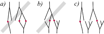
Figure 6: Schematic view of the contribution entering the quasieikonal amplitude in the stochastic approach. Only graphs of type $c)$ contribute.

As the next step we establish a link of the triple Reggeon coupling, $r_{{\scriptscriptstyle 3P}}=\lambda\sqrt{\epsilon}$ in our notations, with the relevant quantities used in fits to the experimental data by different groups (see [11], [12], [13]). To do this we write explicitly the expression for the diffractive cross section in the lowest order in parton splitting, which is expressed via the single triple interaction contribution to the amplitude (see fig.5c). Within the stochastic model we start with the contribution to the amplitude in the Schwimmer approximation with $\alpha^{\prime}\neq 0$ which is first order in $r_{3P}$. The Schwimmer approximation implies eikonal vertices for the target and $m_{2}=\nu=0$. In this case it is straightforward to write down a solution to the set of equations (43) of [3] for the inclusive distribution. The convolution of $f_{2}(Y,b_{1},b_{2})$ with the particle – two Pomeron vertex gives the stochastic model expression for the amplitude in the impact parameter representation:

$$T_{3P}(Y,b)\equiv\int_{y_{\rm min}}^{Y}dy\tilde{T}_{3P}(y,Y;b)=\\ -\lambda\epsilon^{2}N_{A\phantom{\widetilde{A}\!\!\!\!}}N_{\tilde{A}}^{2}\int_{y_{\rm min}}^{Y}dy\int d^{2}b_{1}d^{2}b_{0}d^{2}b_{2}d^{2}b_{2}^{\prime}\,p_{A}({\bf b}_{1})G(y;{\bf b}_{0}-{\bf b}_{1})\\ \times G(Y-y;{\bf b}_{2}-{\bf b}_{0})G(Y-y;{\bf b}_{2}^{\prime}-b_{0})p_{\tilde{A}}({\bf b}-b_{2})p_{\tilde{A}}({\bf b}-b_{2}^{\prime})~{}.$$ (45)

Its discontinuity which corresponds to the intermediate state with rapidity gap $y$ (diffractive dissociation) is of the positive sign and double magnitude. The corresponding single diffractive cross section is

$$\frac{d\sigma^{\rm SD}}{dy_{M}} \equiv M^{2}\frac{d\sigma^{\rm SD}}{dM^{2}}=-2\int d^{2}b\,\tilde{T}_{3P}(y_{M},Y;b)=$$

$$=r_{{\scriptscriptstyle 3P}}\beta_{A\phantom{\widetilde{A}\!\!\!\!}}(0)e^{\Delta(Y-y)}\int\frac{dt}{2\pi}\,\left(\beta_{\tilde{A}}(t)\right)^{2}e^{2(\Delta+\alpha^{\prime}t)y}~{}.$$ (46)

where $y_{M}=Y-y=\ln(M^{2}/s_{0})$.

We make direct comparison of (38) and (46) with the corresponding definitions of [11] ($r_{K}$), [12] ($r_{G}$) and [13] ($r_{L}$) to find out that

$$r_{{\scriptscriptstyle 3P}}=\sqrt{\pi}\,r_{K}=\sqrt{\frac{1}{2\pi}}\,r_{L}=\frac{r_{G}}{2\sqrt{2}}~{}.$$

5.2 The cross sections.

In order to estimate the role of loop corrections it is instructive to compare our calculations with one of the realistic fit to the experimental data. Our aim is not to fit the data better – we want to estimate the relative contribution of the loop diagrams at realistic parameter values. As a starting point for the numerical calculation of the cross section we take a quasieikonal fit to data according to [14] with

$$T(Y,{\bf b})=\sum_{n=1}^{\infty}\frac{(-C)^{n-1}}{n!}\left(T_{P}(Y,{\bf b})\right)^{n}~{},$$ (47)

where

$$T_{P}(Y,{\bf b})=\frac{g_{0}^{2}\exp(\Delta Y)}{R_{P}^{2}+\alpha^{\prime}Y}\exp[-\tfrac{1}{4}b^{2}/(R_{P}^{2}+\alpha^{\prime}Y)].$$ (48)

The fit has a Gaussian parametrization of the Pomeron–particle vertex. The parameters of the fit are as follows:

$$\Delta =0.12~{},$$

$$g_{0}^{2} =2.14~{}\text{GeV}^{-2}\approx 0.083~{}\mathrm{fm}^{2}~{},$$

$$\alpha^{\prime}_{P} =0.22~{}~{}\mathrm{GeV}^{-2}\approx 0.0085~{}\mathrm{fm}^{2}~{},$$ (49)

$$R_{P}^{2} =3.30~{}\mathrm{GeV}^{-2}\approx 0.128~{}\mathrm{fm}^{2}~{},$$

$$C =1.5~{}.$$

We take initial parton distribution in the transverse plane according to this fit in the Gaussian form accounting for a different amplitude normalization in [14] :

$$p_{p}({\bf b})=\frac{1}{4\pi R^{2}}\exp\left[-\frac{b^{2}}{2R^{2}}\right]$$

and the factorial moments of the parton number distribution as

$$\mu_{s}=\left(\bar{N}\right)^{s}C^{\frac{s-1}{2}};\quad\bar{N}=\frac{2g_{0}}{a}$$

We fix the Pomeron intercept $\Delta=\lambda-m_{1}=0.12$ and the triple Pomeron coupling $r_{{\scriptscriptstyle 3P}}=\lambda\sqrt{\pi a^{2}}=0.087$ GeV^-1 which corresponds to the value $r_{K}=0.05~{}\mathrm{GeV}^{-1}$ from [11] in our normalization.

Our aim is to illustrate dependencies of the cross sections on the parton size (linkage distance) $a$ and quartic coupling $\chi$. Following the relations outlined in table 1 and throughout the section we define several sets of the partonic scheme parameters which correspond to the parameter set (49) and differ with transverse size of the parton $a$ and the values of the quartic coupling $\chi$. We fix the parton size values at the level of 5% and 10% of the proton radius. The quartic couplings depending on relation between $\lambda$ and $m_{2}$ for the sets are $\chi_{1}=\chi_{4}=0.0005569$ fm², $\chi_{2}=0.0002785$ fm², $\chi_{3}=0.0011134$ fm². The sets of parameters are presented in table 3.

Table 3: Parameters used for the full calculation within the stochastic scheme. For all the sets $R=0.36$ fm and $D=0.008538$ fm² are taken.

Set $a$, fm $\lambda$ $m_{1}$ $m_{2}$ $\nu$ $\bar{N}$ 1 0.018 0.54722 0.42722 0 1.09488 32.02 2 0.018 0.54722 0.42722 0.54722 0 32.02 3 0.036 0.27361 0.15361 0 0.54722 16.01 4 0.036 0.27361 0.15361 0.27361 0 16.01

The results of the full calculation are presented in figure 7. As one can see, Pomeron interaction leads to a certain shadowing in the amplitudes and hence slows down the cross section growth compared to the quasieikonal approximation. The value of the cross section is mainly defined by the regularization scale (parton size $a$) and not by the value of the quartic coupling, the same as for the Pomeron propagator. We have also checked numerically the independence of the result on the linkage point and found it to hold within 2% accuracy. We have also verified that the quasieikonal approximation is reproduced numerically in our computation once we impose restrictions on the parton sets evolution and their linkage procedure as described in section 5.1.

It is possible by changing parameters to bring the results of the full calculation close to the quasieikonal fit to data. We did so by leaving all the coupling the same and increasing the intercept value simply reducing $m_{1}$. As one can see in the fig. 7 changing the value of $\Delta=\lambda-m_{1}$ to 0.165 brings the full calculation results close to the original quasieikonal fit ($\Delta=0.12$). The curves for the derived sets with $\Delta=0.165$ are additionally marked with an asterix (1*, 2*, 3*, 4*) with respect to the original sets with $\Delta=0.12$. The change in the value of the quartic coupling $\chi$ has a minor influence on the cross section, much less than a change in the regularization scale (parton size) $a$.

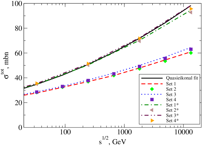
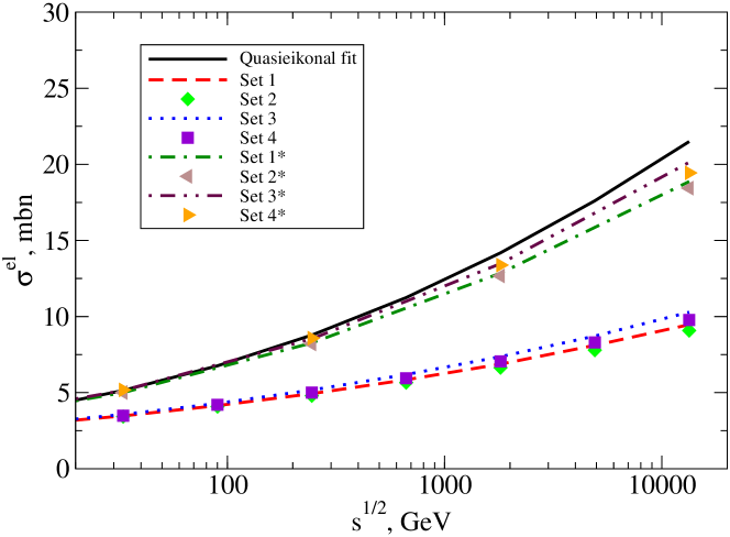
Figure 7: Total and elastic cross sections; full calculation compared to the quasieikonal fit [14].

The same as for the intercept value 1.12, the quartic coupling value has a minor influence on the values of the cross sections. For the energies reachable in the nearest future changing quartic coupling by a factor of 2 amounts to less than 5% change in the cross sections.

6 Conclusion.

We developed a numerical realization of the RFT which allows to obtain the exact value of scattering amplitude taking all loops into account using the equivalence between the Reggeon Field Theory with Pomeron scattering term and parton stochastic model (reaction-diffusion approach). Unlike other calculations with account of loops for no-zero Pomeron slope [13, 15, 16] our aproach does not involve infinite number of fine-tuned couplings for transitions of $m$ into $n$ Pomerons where results depend strongly on the chosen $n,m$ dependencies of the vertices. Our calculations includes triple and quartic couplings only and, to our knowledge, is the first numerical all-loop calculation for the case of non zero slope. This calculation possesses the expected properties of the approach: boost invariance and projectile-target symmetry. Moreover, it gives the exact amplitude as an expansion in the number of the Pomeron exchanged at a given rapidity value $y$ which provides an straightforward opportunity of calculating the quantities which involve this expansion, such as multiplicity distribution in the narrow rapidity interval.

The stochastic model has several parameters, most of them have direct correspondence within RFT and are fixed through its couplings. One of the two parameters which are not fixed at once is the parton interaction distance $a$. It is equivalent to the ultraviolet cutoff or the Pomeron size for the calculations within the RFT thus playing a role of the RFT renormalization scale. Another parameter is the ratio of parton fusion to parton annihilation probabilities. This ratio defines the relative value of triple and quartic Pomeron couplings and up to our knowledge there are no experimental constraints on its value yet. However, as we show numerically the role of the quartic coupling in the RFT with the slope $\alpha^{\prime}$ distinct from zero is negligible for the asymptotic behaviour of the amplitudes and the cross sections within the reach of numerical computations. This is unlike the case of the zero slope.

As an illustration of use of our approach we compute the total and elastic proton-proton cross sections in the approximation of quasieikonal proton-Pomeron vertices. Comparison of the full calculation with the quasieikonal fit shows that for the relevant energy range the full account of the Pomeron interactions can be effectively imitated in the quasieikonal approximation by reducing the intercept from $\Delta=0.165$ to $\Delta=0.12$.

We hope that our study will be helpful in understanding the role of relative value of the Pomeron loop contribution in high energy hadronic scattering.

References

- [1] V. N. Gribov, Sov. Phys. JETP 26, 414 (1968) [Zh. Eksp. Teor. Fiz. 53, 654 (1967)].
- [2] P. Grassberger, K. Sundermeyer, Phys. Lett. B77 (1978) 220.
- [3] K. G. Boreskov, In *Olshanetsky, M. (ed.) et al.: Multiple facets of quantization and supersymmetry* 322-351. [hep-ph/0112325].
- [4] S. Bondarenko, L. Motyka, A. H. Mueller, A. I. Shoshi, B.-W. Xiao, Eur. Phys. J. C50 (2007) 593-601.
- [5] G. P. Salam, Nucl. Phys. B461 (1996) 512-538. [hep-ph/9509353].
- [6] E. Avsar, G. Gustafson, L. Lonnblad, JHEP 0701 (2007) 012. [hep-ph/0610157].
- [7] H. Minc. Permanents. Reading, MA: Addison-Wesley, 1978.
- [8] D. Amati, L. Caneschi, R. Jengo, Nucl. Phys. B101 (1975) 397.
- [9] M. A. Braun, G. P. Vacca, Eur. Phys. J. C50 (2007) 857-869. [hep-ph/0612162].
- [10] H. D. I. Abarbanel, J. B. Bronzan, R. L. Sugar, A. R. White, Phys. Rept. 21 (1975) 119-182.
- [11] A. B. Kaidalov, Phys. Rept. 50 (1979) 157-226.
- [12] K. A. Goulianos, Phys. Lett. B358 (1995) 379-388. [hep-ph/9502356]. K. A. Goulianos, J. Montanha, Phys. Rev. D59 (1999) 114017. [hep-ph/9805496].
- [13] E.G.S. Luna, V.A. Khoze, A.D. Martin and M.G. Ryskin, Eur. Phys. J. C59 (2009) 1.
- [14] K.A. Ter-Martirosyan, Sov. J. Nucl. Phys. 44 (1986) 817 [Yad. Fiz. 44 (1986) 1257].
- [15] A. B. Kaidalov, M. G. Poghosyan, [arXiv:0909.5156 [hep-ph]].
- [16] S. Ostapchenko, Phys. Rev. D81 (2010) 114028. [arXiv:1003.0196 [hep-ph]].