X-ray Time Lags in TeV Blazars

Abstract

We use Monte Carlo/Fokker-Planck simulations to study the X-ray time lags. Our results show that soft lags will be observed as long as the decay of the flare is dominated by radiative cooling, even when acceleration and cooling timescales are similar. Hard lags can be produced in presence of a competitive achromatic particle energy loss mechanism if the acceleration process operates on a timescale such that particles are slowly moved towards higher energy while the flare evolves. In this type of scenario, the $\gamma$-ray/X-ray quadratic relation is also reproduced.

1 Introduction

One of the most interesting and least studied in details aspects of TeV blazars variability is that of time lags between variations at different energies in the X-ray band. The results of the time delay analysis of the X-ray sub-bands include all three possibilities: soft lag, hard lag, and no lag. (e.g. Rebillot et al., 2006; Fossati et al., 2000; Brinkmann et al, 2005).

One the best modeling works addressing the issue of time lags in the synchrotron emission remains that by Kirk and collaborators (1998). They assumed that most of the jet emission, certainly the more highly variable component, is produced by shocked plasma and modeled it as a moving shock and its immediate downstream region. Their work, similarly to most more recent modeling, did not take into account the light travel times effects (LTTE) within the emission region and with respect to the observer, which can modify significantly the phenomenology (e.g., Chen et al., 2010). LTTE are important to blazars but very difficult to calculate in traditional ways of solving the radiative transfer equation.

Here we present preliminary results of a more advanced simulation code that allows us to include LTTE, and begin to analyze the scenarios and conditions that can lead to different time-lag signatures. The results are obtained with our Monte Carlo/Fokker-Planck radiation transfer code described in (Chen et al., 2010). The Monte Carlo methods allows to track the trajectories of individual (pseudo)photons, thus accounting naturally for all the LTTEs. We handle the electrons as populations with densities and distributions, and use the Fokker-Planck equation to solve for their time evolution. The acceleration, cooling, injection and achromatic loss of electrons are all realized through the Fokker-Planck equation. The geometry of the plasma blob is assumed to be cylindrical as shown in Fig. 1, left.

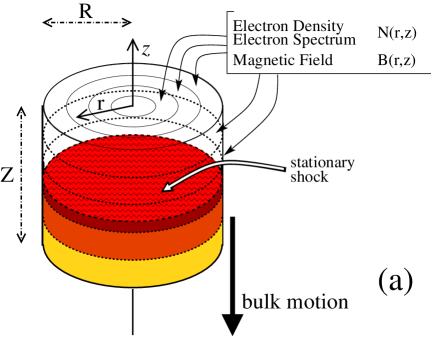
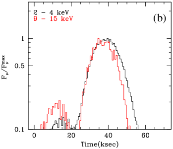
Figure 1: (a): The geometry of the model. The volume is divided in the $r$ and $z$ directions in zones with their own electron distribution and magnetic field. We also schematically show the setup for the variability of the simulations with a shock. The hatched layer represents a stationary shock. The blob moves downward and crosses the shock front. Zones that crossed the shock at earlier times have had some time to radiate the newly injected energy and are plotted in lighter color shades. (b): The light curves produced by the scenario #2. During the flare rise both bands vary together, but in the decay phase the harder band drops more rapidly yielding a soft lag.

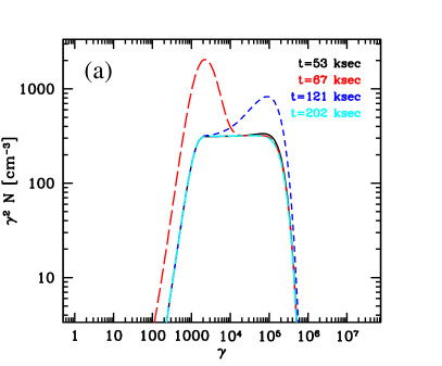
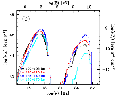
Figure 2: For case # 4. (a): evolution of the electron spectrum in one of the blob zones. (b): SEDs. In both panels, the time sequence is: black, red, blue, cyan. Times are in the observer’s frame. Model parameters: $B=0.1$ G, $\delta=33$, sizes: $z=1.33\times 10^{16}$ cm, $r=10^{16}$ cm, $n_{e}=0.4$ cm^-3, injection rate $q=3.17\times 10^{39}$ erg/s without shock increasing by a factor of 8 with the shock. Time-scales: acceleration $t_{\rm acc}=z/c$, and achromatic loss $t_{\rm loss}=z/c$. The shock begins to cross the blob at $t=60$ ks.

2 Summary of four flare scenarios

We have tested 4 different scenarios:

#1: Homogeneous, steady rate, injection of high energy particles with power law distribution. The flare is caused by an increase/decrease of the maximum electron energy $\gamma_{\rm max}$, following an exponential (symmetric) time evolution.

#2: Homogeneous mild diffusive particle acceleration mechanism is active in the blob for a set duration, after which the evolution is purely radiative.

#3: Rapid electron acceleration locally as the shock crosses the blob, followed by a purely radiative evolution.

#4: The shock causes a local burst of injection of medium energy electrons ($\gamma=10^{3}$, with narrow Gaussian spectrum), which happens in a blob where it a steady diffusive (slow-ish) acceleration mechanism is present. The particle cooling is not purely radiative, but it includes an achromatic energy loss process which is the main factor controlling the flare decay.

The physical explanation for the mild diffuse acceleration in the blob can be shear acceleration (e.g., Rieger & Duffy, 2004), while the injected medium energy electrons may come from the stochastic particle acceleration (e.g., Katarzyński et al. 2006). The achromatic energy loss can be thought of as caused by adiabatic expansion or particle escape.

The first three models failed to produce a X-ray hard lag (e.g., see the light curves for #2 in Fig. 1b). In cases #1 and #2 the soft X-ray variation leads the hard X-ray one, but in all these models the spectral evolution during the flare decay is controlled by radiative cooling, hence it always propagates from high to low energy, yielding a soft lag (even after smearing by LTTEs).

The more complex fourth scenario successfully produced a hard X-ray lag (see Fig. 2b for SEDs and Fig. 3a for light curves). This model is similar to the second model, in the sense that in both the mild particle acceleration slowly moves the electrons from low/medium energy to high energy, providing the hard lag when the flux increases. The crucial difference is that the decay of the flare in the fourth model is controlled by achromatic energy loss, which eliminates the emergence of the soft lag. Radiative cooling is balanced by particle acceleration, so it does not have much control on the flux and spectral change. The left panel of Fig. 3 shows how the electron energy distribution evolves in this model.

A potential problem in this model is that the optical flux shows a large, and early, variation, as seen in Fig. 3a, which is not usually observed. This problem can be mitigated by the possible presence of additional emission by other regions of the jet having lower energy particles (e.g. Ushio et al., 2009; Krawczynski, Coppi & Aharonian, 2002; Chen et al., 2010). This emission can have a SED peaking closer to the optical band and not very luminous in X-rays, thus diluting significantly the observed optical variations with respect to their intrinsic magnitude, without affecting much our view of the flaring emission in X-ray.

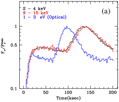
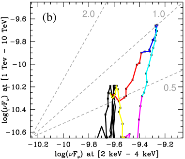
Figure 3: Case #4. (a): Light curves in three energy bands. (b): $\gamma$-ray vs. X-ray flux correlation. Colors represent different times: black ($<100ks$), red ($100-120$ ks), blue ($120-140$ ks), cyan ($140-160$ ks), magenta ($160-180$ ks), yellow ($>180$ ks).

Scenario #4 also yields a quadratic relation between $\gamma$-ray and X-ray fluxes in both the raising and decay phases of the flare (see Fig. 3b), a feature frequently observed in TeV blazars that has proved to be challenging to model (Fossati et al., 2008). Our previous efforts with flare evolution dominated by radiative cooling could only produce the quadratic relation for the flare rising phase (Chen et al., 2010). Again the crucial element here is the adiabatic energy loss mechanism, because it affects at the same time the medium energy electrons that emit the seed photons and the high energy electrons that inverse Compton scatter them.

References

- [1] Brinkmann, W. et al. 2005, A&A, 443, 397
- [2] Chen, X., Fossati, G., Liang, E., & Böttcher, M. 2010, MNRAS, submitted
- [3] Fossati, G. et al. 2000, ApJ, 541, 153
- [4] Fossati, G. et al. 2008, ApJ, 677, 906
- [5] Katarzyński, K. et al. 2006, A&A, 453, 47
- [6] Kirk, J. G., Rieger, F. M., & Mastichiadis, A. 1998, A&A, 333, 452
- [7] Krawczynski, H., Coppi, P. S., & Aharonian, F. 2002, MNRAS, 336, 721
- [8] Rebillot, P. F. et al. 2006, ApJ, 641, 740
- [9] Rieger, F. M., & Duffy, P. 2004, ApJ, 617, 155
- [10] Ushio, M. et al. 2009, ApJ, 699, 1964