Diffusion coefficient of an inclusion in a liquid membrane supported by a solvent of arbitrary thickness

Abstract

The diffusion coefficient of an inclusion in a liquid membrane is investigated by taking into account the interaction between membranes and bulk solvents of arbitrary thickness. As illustrative examples, the diffusion coefficients of two types of inclusions - a circular domain composed of fluid with the same viscosity as the host membrane and that of a polymer chain embedded in the membrane are studied. The diffusion coefficients are expressed in terms of the hydrodynamic screening lengths which vary according to the solvent thickness. When the membrane fluid is dragged by the solvent of finite thickness, via stick boundary conditions, multiple hydrodynamic screening lengths together with the weight factors to the diffusion coefficients are obtained from the characteristic equation. The condition for which the diffusion coefficients can be approximated by the expression including only a single hydrodynamic screening length are also shown.

I Introduction

Recent advances in experimental techniques have made the direct observation of the Brownian motion of $\mu$m sized objects in membranes using microscopy and imaging a routine process Tanaka-07; yanagisawa-07; cicuta-07; kaizuka-04; reitz-01; gambin-06; Aliaskarisohi. As a result, diffusion coefficients can be measured accurately and it is now possible to address the issue of the differences between Brownian motion of macromolecules embedded in membranes in various environments.

Vesicles with sizes of the order of $10$ $\mu$m are frequently used in experiments while the typical distance of a supported membrane from the substrate is of the order of $20$ Å Tanaka-07; yanagisawa-07. Obviously, in both these general cases the coupling of membrane with its environment are very different and hence it will influence the Brownian motion of inclusions. In this paper, we investigate the influence of solvent environments on diffusion of an inclusion embedded in a membrane. In the biological context, there are many examples of membranes coming in contact with a solvent of various depth such as in tissues.

Biological membranes can be regarded as two-dimensional (2D) viscous fluids. An important feature of membranes as a transport media is that they are not purely isolated izuyama-88; suzuki-89; evans-88. Liquid membranes are coupled to surrounding solvents by interaction of polar head groups of lipid molecules with solvents; they form quasi-2D systems coupled to three-dimensional (3D) solvents. The coupling to the surrounding environments induces the momentum exchange between the membrane and the solvents. The influence of the momentum exchange on the Brownian dynamics has been theoretically investigated by introducing a phenomenological coupling constant or simplifying the solvents flow saffman-75; saffman-76; izuyama-88; suzuki-89; evans-88; hughes-81; seki-93; sanoop-drag-10; Petrov-08; komura-95. These studies have also been extended to investigate the concentration fluctuations seki-07; Tserkovbyak-06; inaura-08.

Despite the large number of studies, the Brownian motion of an object in liquid membranes has not yet been fully understood. In a hydrodynamic description, 2D flow in a bilayer membrane can be regarded as viscous and the interaction between liquid membranes and surrounding solvents can be taken into account by the stick boundary condition between them. Diffusion coefficients of macroscopic inclusions embedded in membranes were analytically investigated for a planar membrane surrounded by solvent layers of infinite saffman-75; saffman-76; hughes-81; Petrov-08 or very small thickness izuyama-88; suzuki-89; evans-88; seki-93; sanoop-drag-10; komura-95. These studies revealed that the hydrodynamic flow in a membrane is screened by the solvent drag force and is characterized by a hydrodynamic screening length. When a planar membrane is surrounded by infinite thickness of solvent, it is called the Saffman and Delbrück (SD) hydrodynamic screening length, $\nu^{-1}$, and is given by the ratio between the 2D membrane viscosity $\eta$ and the 3D solvent viscosity $\eta_{s}$, $\nu^{-1}=\eta/\eta_{s}$ saffman-75; saffman-76. (As we shall see below, the dimension of the 2D membrane viscosity is that of 3D solvent viscosity times a length.) In the opposite limit of a thin solvent layer of the thickness $h$, Evans and Sackmann (ES) hydrodynamic screening length given by $\sqrt{h/\nu}$ is appropriate evans-88. In both limits, the diffusion coefficients depend logarithmically on the size of the inclusions as long as the size is smaller than the hydrodynamic screening length. On the other hand, the diffusion coefficients depend on the size of the inclusions very differently when the size of the inclusions exceeds the hydrodynamic screening length. These studies naturally lead to the interest in the hydrodynamic screening length and its influence on the diffusion coefficients when the solvent layer has a finite thickness.

The solvent flow can be varied by changing the solvent thickness. The flow of solvents influences the membrane flow through the stick boundary condition imposed between the membrane and the solvents. As a result, the diffusion coefficients depend on the solvent thickness. The influence of the finite solvent thickness has been recently studied for diffusion of a disk stone-98, concentration fluctuations Haataja-09; inaura-08; sanoop-11, correlated diffusion oppenheimer-09; diamant-09b; oppenheimer-10; sanoop-bulk-10, and polymer diffusion in a membrane Ramachandran-20. Diffusion coefficients of other types of inclusions on membranes levine-04; levine-04b; muthukumar-85; Naji-07; komura-95 or on Langmuir monolayers fischer-04 have also been theoretically calculated. However, the investigation on the influence of finite thickness of solvent was limited to numerical evaluation of the diffusion coefficients, where the dependence of the hydrodynamic screening length on the solvent thickness was not completely elucidated oppenheimer-09; diamant-09b; Ramachandran-20; inaura-08; Haataja-09; sanoop-bulk-10; stone-98; sanoop-11; oppenheimer-10. In this paper, the relation between the diffusion coefficients and the hydrodynamic screening lengths are throughly investigated for an arbitrary thickness of the solvent layers on the basis of the analytical expression on the hydrodynamic screening lengths.

The relation between the diffusion coefficients and the hydrodynamic screening lengths can be shown in a straight-forward manner for a polymer embedded in a membrane by the Zimm model, where the equilibrium average of the hydrodynamic interactions is performed in 2D komura-95; muthukumar-85; Ramachandran-20. The multiple hydrodynamic screening lengths are then found for the finite solvent thickness. The diffusion coefficients are expressed by the weighted sum; each term in the sum is a product of the weight factor and the function of the dimensionless size of the polymer normalized by each hydrodynamic screening length. On the basis of the analytical expression, the condition that the diffusion coefficient is approximately represented solely by the ES hydrodynamic screening length can be discussed in detail. We show that the diffusion coefficient cannot be approximated by the ES hydrodynamic screening length when both $\nu^{-1}=\eta/\eta_{s}$ and the size of the macromolecule are smaller than the solvent thickness.

Essentially the same relation between the diffusion coefficients and the hydrodynamic screening lengths is obtained for diffusion of a circular liquid domain with the same viscosity as that of the host membrane. The diffusion coefficient of a circular liquid domain embedded in a membrane has been studied in relation to recently proposed raft model, where rafts are formed by sphingomyelin and cholesterol rich liquid domains simons-97; brown-98; klingler-93; oradd-05; cicuta-07; yanagisawa-07; kenworthy-04; Aliaskarisohi. It is believed that rafts undergo lateral Brownian motion within a bilayer membrane and act as platforms for protein association and signaling brown-98. Previously, the diffusion coefficient of a circular liquid domain of arbitrary size was derived in the limit of infinite depth of solvent layer or the limit of small depth of solvent layer DeKoker; sanoop-drag-10; Fujitani; Aliaskarisohi. In this paper, the results are generalized for the arbitrary thickness of solvent layers. The diffusion coefficient is obtained as a simple integral which can be expressed again as the sum of the terms given by functions of the same hydrodynamic screening lengths multiplied by the same weight factors as those for the polymer diffusion coefficients.

In Sec. II, the membrane hydrodynamics is reviewed. The diffusion coefficient of a polymer embedded in a membrane is obtained in Sec. III. In Sec. IV, the relation between hydrodynamic screening length and the solvent thickness is discussed. The diffusion coefficient of a liquid domain in a membrane is obtained in Sec. LABEL:Calculation. Finally, the last section is devoted to conclusions.

II Hydrodynamic flow in a membrane and solvent

As shown in Fig. 1, we consider the situation where the liquid membrane is supported by a bulk solvent on the solid substrate. The situation where the membrane is also supported by a solvent from above will be considered in Sec. VI. We denote the 2D flow in the membrane by ${\bf v}({\bf r})$ where ${\bf r}=(x,y)$ represents a position within the plane of the membrane. The membrane is regarded to be incompressible,

$${\bf\nabla}\cdot{\bf v}({\bf r})=0.$$ (1)

Here $\nabla$ is a differential operator in the 2D Euclidean space. The viscous flow in the membrane can be expressed by the Stokes equation in 2D,

$$\eta\nabla^{2}{\bf v}({\bf r})-\nabla p({\bf r})+{\bf f}_{\rm s}({\bf r})=0,$$ (2)

where $\eta$ is the 2D membrane viscosity, $p({\bf r})$ the in-plane pressure, and ${\bf f}_{\rm s}({\bf r})$ the in-plane force exerted on the membrane from the solvent. The last quantity can be obtained when the solvent fluid velocities are determined. The stress tensor of the liquid membrane is given by

$$\sigma_{\alpha\beta}({\bf r})=-p({\bf r})\delta_{\alpha\beta}+\eta[\partial_{\alpha}v_{\beta}({\bf r})+\partial_{\beta}v_{\alpha}({\bf r})],$$ (3)

where $\delta_{\alpha\beta}$ is the Kronecker delta, and $\alpha$, $\beta$ are $x$, $y$. Then Eq. (2) can be represented in terms of the stress tensor as,

$${\rm div}\,{\bm{\sigma}}+{\bm{f}}_{\rm s}({\bm{r}})=0,$$ (4)

where $({\rm div}\,{\bm{\sigma}})_{\alpha}=\sum_{\beta}\partial\sigma_{\alpha\beta}/\partial x_{\beta}$.

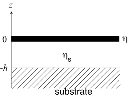
Figure 1: Schematic picture showing a planar liquid membrane with 2D viscosity $\eta$ located at $z=0$. It is supported on a solvent with 3D viscosity $\eta_{\rm s}$. A substrate is located at $z=-h$ bounding the solvent.

As shown in Fig. 1, the membrane is located in the plane at $z=0$. The solvent velocities ${\bf v}^{(3)}({\bf r},z)$, satisfy the incompressibility condition

$$\tilde{{\bf\nabla}}\cdot{\bf v}^{(3)}({\bf r},z)=0,$$ (5)

where $\tilde{\nabla}$ represents a differential operator in the 3D Euclidean space. We denote the 3D viscosity of the solvent as $\eta_{\rm s}$, and the solvent flow also obeys the 3D Stokes equation,

$$\eta_{\rm s}\tilde{{\bf\nabla}}^{2}{\bf v}^{(3)}({\bf r},z)-\tilde{{\bf\nabla}}p^{(3)}({\bf r},z)=0,$$ (6)

where $p^{(3)}({\bf r},z)$ represents the pressure of the solvent. The solvent is supported on the substrate which is located at $z=-h$. The no-slip boundary condition is imposed at $z=-h$ as well as between the membrane flow and the solvent flow. Through this boundary condition, the surrounding solvent exerts a drag force on the liquid membrane.

The drag force in Eq. (2) can be expressed as ${\bf f}_{\rm s}=-({\bf I}-\hat{{\bf e}}_{z}\hat{{\bf e}}_{z})\cdot{\bf\sigma}^{(3)}({\bf r},0)\cdot\hat{{\bf e}}_{z}$, where $\hat{{\bf e}}_{z}$ is the unit vector along the $z$-axis. The tensorial component of ${\bf I}$ is given by $\delta_{ij}$, and ${\bf I}-\hat{{\bf e}}_{z}\hat{{\bf e}}_{z}$ denotes the projection to the in-plane space. The stress tensor of solvent is given by

$$\sigma_{ij}^{(3)}({\bf r},z)=-p^{(3)}({\bf r},z)\delta_{ij}+\eta_{\rm s}[\tilde{\partial}_{i}v_{j}^{(3)}({\bf r},z)+\tilde{\partial}_{j}v_{i}^{(3)}({\bf r},z)],$$ (7)

where $i$, $j$ denote $x$, $y$, $z$.

Using the stick boundary conditions at $z=0$ and $z=-h$, we solve the hydrodynamic equations from Eq. (5) to Eq. (6) to obtain ${\bf f}_{\rm s}$. In the Fourier space, ${\bf f}_{\rm s}$ is calculated to be inaura-08; fischer-04; lubensky-96

$${\bf f}_{\rm s}[{\bf k}]=-\eta_{\rm s}k\coth(kh){\bf v}[{\bf k}],$$ (8)

where ${\bf k}=(k_{x},k_{y})$ and $k=|{\bf k}|$. The real space velocity field of the membrane flow ${\bf v}({\bf r})$ can be expressed as

$${\bf v}({\bf r})=\int\frac{{\rm d}^{2}k}{(2\pi)^{2}}\,{\bf v}[{\bf k}]\exp(i{\bf k}\cdot{\bf r}).$$ (9)

The Fourier space mobility tensor ${\bf G}[{\bf k}]$ associated with the velocity field is given by fischer-04; lubensky-96; inaura-08

$$G_{\alpha\beta}[{\bf k}]=\frac{1}{\eta[k^{2}+\nu k\coth(kh)]}\left(\delta_{\alpha\beta}-\frac{k_{\alpha}k_{\beta}}{k^{2}}\right).$$ (10)

In order to calculate diffusion coefficients, the mobility tensor in Fourier space should be transformed into real space. Previously, the inverse Fourier transform of the mobility tensor was analytically performed only in the limits of infinite or zero thicknesses of a solvent layer. In the next section, the inverse Fourier transformation of the mobility tensor is analytically performed for an arbitrary thickness of a solvent.

III Diffusion coefficient of a 2-dimensional polymer chain

As an illustrative example for the influence of finite thickness of solvent on the diffusion coefficient of a macromolecule embedded in a 2D planar membrane, we consider the diffusion of a polymer chain confined in the membrane muthukumar-85; komura-95; Ramachandran-20. Previously, the influence of the solvent on diffusion coefficients is analytically investigated only in the limits of very thin or infinite thicknesses of solvent layers. In these works, the hydrodynamic screening length is a key quantity in characterizing the screening of the flow of membrane by the presence of solvent layers. The influence of finite thickness of solvent was investigated by numerically evaluating the inverse Fourier transform of the mobility tensor, where the hydrodynamic screening length was not even defined. In this section, the hydrodynamic screening lengths are obtained from an analytical equation for arbitrary thickness of solvent layer.

The conformation of a 2D polymer chain embedded in a 2D membrane is represented by $N$ beads with position vectors, $\{{\bf R}_{n}\}=({\bf R}_{1},\ldots,{\bf R}_{N})$, under the potential energy,

$$U=\frac{k_{\rm B}T}{b^{2}}\sum_{n=2}^{N}({\bf R}_{n}-{\bf R}_{n-1})^{2},$$ (11)

where $b$ is the Kuhn length doi-edwards. The mobility tensor associated with the beads is given by the inverse Fourier transform of Eq. (10) as

$$G_{\alpha\beta}\left({\bf R}_{n}-{\bf R}_{m}\right)=\int\frac{{\rm d}^{2}k}{(2\pi)^{2}}\,G_{\alpha\beta}[{\bf k}]\exp\left[i{\bf k}\cdot\left({\bf R}_{n}-{\bf R}_{m}\right)\right].$$ (12)

Within the pre-averaging approximation doi-edwards, the polymer diffusion coefficient is expressed as

$$D_{\rm poly}=k_{\rm B}T\int_{0}^{N}\frac{{\rm d}n}{N}\int_{0}^{N}\frac{{\rm d}m}{N}\,g(n-m),$$ (13)

where $g(n-m)$ is the isotropic component of mobility tensor $G_{\alpha\beta}\left({\bf R}_{n}-{\bf R}_{m}\right)$ Ramachandran-20. By using Eq. (12), two analytical expressions for the diffusion coefficients have been derived from Eq. (13) in the limits of very thin or infinite thickness of solvent layers  komura-95; Ramachandran-20. Here, we investigate the diffusion coefficient by keeping the finite depth of the solvent layer without taking the limits. By expanding $1/[k+\nu\coth(kh)]$ in partial fractions, we note the general relation John-50

$$\int_{0}^{\infty}{\rm d}k\,\frac{f(k)}{k+\nu\coth(kh)}=\sum_{j=1}^{\infty}C_{j}\int_{0}^{\infty}{\rm d}k\,\frac{kf(k)}{k^{2}+\kappa_{j}^{2}},$$ (14)

where $f(k)$ is an arbitrary function, $\kappa_{j}$ and $C_{j}$ will be later given by Eqs. (16) and (17), respectively. By introducing Eq. (14) into Eqs. (12) and (13), we obtain,

$$g(n-m) =-\sum_{j=1}^{\infty}C_{j}\frac{1}{8\pi\eta}\exp\left(\frac{1}{4}b^{2}\kappa_{j}^{2}|n-m|\right)$$

$$\quad\quad\quad\quad\times{\rm Ei}\left(-\frac{1}{4}b^{2}\kappa_{j}^{2}|n-m|\right),$$ (15)

where ${\rm Ei}(-z)$ is the exponential integral abram-stegun.

In the real space, the mobility tensor is expressed in terms of an infinite number of characteristic lengths, $\kappa_{j}^{-1}$, where $\kappa_{j}$ is determined by the following characteristic equation

$$\cot(\kappa_{j}h)=\frac{\kappa_{j}}{\nu}.$$ (16)

All the roots of the equation are given by $\kappa=\pm\kappa_{j}$ with $j=1,2,\cdots$. The characteristic lengths relative to $h$, $1/(\kappa_{j}h)$, depend on $\nu h$ given by the viscosity ratio $\nu=\eta_{s}/\eta$, and represent the screening of hydrodynamic flow in 2D membrane due to the presence of the solvent. The contribution of each screening length is weighted by the factor

$$C_{j}=\frac{2\nu}{h\kappa_{j}^{2}+h\nu^{2}+\nu}.$$ (17)

Using Eq. (15), the diffusion coefficient is obtained as

$$D_{\rm poly} =\sum_{j=1}^{\infty}C_{j}\frac{k_{\rm B}T}{4\pi\eta}\frac{1}{\epsilon_{j}^{4}}\Big{[}(1+\epsilon_{j}^{2})(2\ln\epsilon_{j}+\gamma)$$

$$\quad\quad\quad\quad\quad\quad-\epsilon_{j}^{2}-\exp(\epsilon_{j}^{2}){\rm Ei}(-\epsilon_{j}^{2})\Big{]},$$ (18)

where $\gamma=0.5772\cdots$ is Euler’s constant. In the above, we have defined the dimensionless polymer size as $\epsilon_{j}\equiv\sqrt{N}b\kappa_{j}/2=R_{\rm g}\kappa_{j}$, and $R_{\rm g}=\sqrt{N}b/2$ is the radius of gyration for the 2D Gaussian polymer chain.

The limiting expression for $\epsilon_{1}\ll 1$ is

$$D_{\rm poly}\approx C_{1}\frac{k_{\rm B}T}{4\pi\eta}\left[-\ln\epsilon_{1}-\frac{\gamma}{2}+\frac{3}{4}\right].$$ (19)

As will be discussed in the next section, the above expression is close to the exact result under the additional condition of $\nu h<1$ which is needed to replace the sum in Eq. (18) with the term related to $\epsilon_{1}$. When $\epsilon_{1}\gg 1$, Eq. (18) reduces to

$$D_{\rm poly}\approx C_{1}\frac{k_{\rm B}T}{4\pi\eta}\frac{1}{\epsilon_{1}^{2}}\Big{[}2\ln\epsilon_{1}+\gamma-1\Big{]}.$$ (20)

This expression holds regardless of the value of $h$ as long as it is finite. The sum in Eq. (18) can be represented by the single dominant term as long as $\epsilon_{1}\gg 1$. However, the additional condition of $\nu h<1$ is required when $\epsilon_{1}\ll 1$, about which we shall discuss in the next section.

IV Hydrodynamic screening length vs. solvent thickness

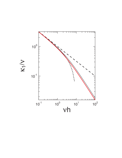
Figure 2: (Color online) The smallest positive values for the inverse of the characteristic lengths against the solvent thickness. Both quantities are normalized by $\nu=\eta_{\rm s}/\eta$. The red thick line represents the smallest positive root of the characteristic equation, Eq. (16), calculated numerically. The long dashed line represents $\kappa/\nu=1/\sqrt{\nu h}$. The short dashed line represents the result of Eq. (23). The thin solid line represents the result of Eq. (22).

If the approximated diffusion coefficient obtained by taking into account only the smallest positive value of $\kappa_{j}$ (denoted by $\kappa_{1}$) reproduce the exact results, then $\kappa_{1}^{-1}$ can be regarded as the effective hydrodynamic screening length.

First, we consider the value of $\kappa_{1}$ which is the inverse of the effective hydrodynamic screening length as long as the higher order ($j\geq 2$) terms can be ignored. We first note the series expansion,

$$x\cot x=1+2\sum_{n=1}^{\infty}\frac{x^{2}}{x^{2}-n^{2}\pi^{2}}.$$ (21)

Since the lowest order term can be estimated as $1+2x^{2}/(x^{2}-\pi^{2})\approx x^{2}/(\nu h)$, the approximate expression for $\kappa_{1}$ turns out to be

$$\kappa_{1}\approx\left(\frac{3\nu h+\pi^{2}-\sqrt{(3\nu h)^{2}+2\nu h\pi^{2}+\pi^{4}}}{2h^{2}}\right)^{1/2}.$$ (22)

In the limit of $\nu h/\pi^{2}<1$, $\kappa_{1}$ can be further approximated as

$$\kappa_{1}\approx\kappa\left(1-\frac{\nu h}{\pi^{2}}\right),$$ (23)

where $\kappa=\sqrt{\nu/h}$ is the inverse of the ES hydrodynamic screening length defined in the limit of $h\rightarrow 0$. In Fig. 2, the smallest positive values for the inverse of the characteristic lengths are presented against the solvent layer thickness, $h$. By increasing the solvent layer thickness $h$, the inverse of the hydrodynamic screening length rapidly decreases as shown in Fig. 2.

Next we consider the condition for which the diffusion coefficient can be characterized by a single hydrodynamic screening length as a good approximation for the exact expression including multiple hydrodynamic screening lengths associated with higher order $\kappa_{j}$. Judging from Eq. (16) and Fig. 3 (a), $\kappa_{j}$ takes discrete values which are almost equally separated. When $\kappa_{1}R_{\rm g}$ is well separated from $\kappa_{2}R_{\rm g}$ and the diffusion coefficient is given by the weighted sum of monotonically decreasing functions of $\kappa_{j}R_{\rm g}$ multiplied by the rapidly decreasing weights, the sum can be well represented by the term associated with $\kappa_{1}R_{\rm g}$ alone. Below, we show that $\kappa_{1}R_{\rm g}$ is well separated from $\kappa_{2}R_{\rm g}$ when $R_{\rm g}>h$ and the weights rapidly decay when $h<1/\nu$.

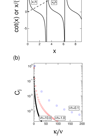
Figure 3: (Color online)

(a) The pictorial solution of the characteristic equation, Eq. (16); $\cot(x)$ against $x$ and $x/(\nu h)$ against $x$ for $\nu h=1$. The cross points of lines are $x_{j}=\kappa_{j}h$. The smallest positive value is $x_{1}$. $\kappa_{1}$ is obtained by $\kappa_{1}=x_{1}/h$ (b) $C_{j}$ against $\kappa_{j}/\nu$. $C_{j}$ represents the weight associated with each hydrodynamic screening length, Eq.(17). Blue squares, red circles and dots represent $\nu h=0.1$, $\nu h=1.0$ and $\nu h=10.0$, respectively.