Testing Skyrme energy-density functionals with the QRPA in low-lying vibrational states of rare-earth nuclei

Abstract

Although nuclear energy density functionals are determined primarily by fitting to ground state properties, they are often applied in nuclear astrophysics to excited states, usually through the quasiparticle random phase approximation (QRPA). Here we test the Skyrme functionals SkM^∗ and SLy4 along with the self-consistent QRPA by calculating properties of low-lying vibrational states in a large number of well-deformed even-even rare-earth nuclei. We reproduce trends in energies and transition probabilities associated with $\gamma$-vibrational states, but our results are not perfect and indicate the presences of multi-particle-hole correlations that are not included in the QRPA. The Skyrme functional SkM^∗ performs noticeably better than SLy4. In a few nuclei, changes in the treatment of the pairing energy functional have a significant effect. The QRPA is less successful with “$\beta$-vibrational” states than with the $\gamma$-vibrational states.

I Introduction

Modern supercomputers are making the quantitative theoretical treatment of nuclear structure increasingly common. In light nuclei, Greens-function Monte Carlo methods Pieper et al. (2004); Pieper and Wiringa (2001) and the no-core shell model Negoita et al. (2010); Vary et al. (2009) yield accurate ab initio results, and in medium-mass nuclei the coupled cluster method Hagen et al. (2007); Dean and Hjorth-Jensen (2004) is proving successful. In nuclei with $A>50$, techniques related to density-functional theory (DFT) Dobaczewski (2010) are the state of the art. Accuracy, at least for ground-state properties, is limited only by the quality of the functionals, which are continually improving Kortelainen et al. (2010).

One advantage of DFT is its applicability to nearly all heavy nuclei. Such flexibility is particularly important for nuclear astrophysics, which attempts to explain the synthesis of all the elements. Another advantage is a natural extension, through the self-consistent quasiparticle random phase approximation (QRPA) to excitations. Excited states are as important as ground states in many nucleosynthetic reactions, and so Goriely et al. Goriely and Khan (2002), for example, used the QRPA to compute radiative neutron capture in a wide range of nuclei. Such calculations, however, have generally ignored deformation, or treated it in a crude way. The logical next step is to take the effects of deformation into account in a self-consistent fashion.

Fortunately, self-consistent QRPA calculations in heavy deformed nuclei are now becoming possible. Recently, we developed a scaled parallel Skyrme-QRPA code Terasaki and Engel (2010) for arbitrary axially-deformed (parity conserving) even-even nuclei. Our code is one of the few Péru et al. (2011) to treat heavy deformed nuclei in the QRPA without simplification. (For other calculations, including those in lighter nuclei and those in the RPA, the spherical QRPA, and separable approximations, see the work cited in Ref. Terasaki and Engel (2010) and, e.g., the more recent Ref. Yoshida and Nakatsukasa (2011).) In this paper, we present calculations with two Skyrme energy-density functionals of properties of low-energy vibrational states in rare-earth nuclei. As promised in Ref. Terasaki and Engel (2010), we discuss the performance of both the functionals and the QRPA.

In Sec. II below we list the nuclei that we explore and present technical information about our calculations. In Sec. III we show results for $\gamma$-vibrational states and discuss the performance of the Skyrme QRPA, which we compare with methods used in earlier calculations. Sec IV treats “$\beta$-vibrational” states briefly, and Sec. V is a conclusion. An appendix presents equations for two-body matrix elements of the Coulomb-direct interaction and discusses computational efficiency.

II Selection of Nuclei and Method of Calculation

The vibrational states we examine are all in rare-earth nuclei. The advantage of this region of the isotopic chart is the abundance of reliable experimental data Oshima et al. (1995); Sugawara et al. (1993); Fahlander et al. (1992a, b); Kotliński et al. (1990); Burke et al. (1988); Ichihara et al. (1987); Walker (1983); Ronningen et al. (1982); Cresswell et al. (1981); McGowan and Milner (1981); Riedinger et al. (1979); McGowan et al. (1978); Wollersheim and Th. W. Elze (1977); Ronningen et al. (1977); Reich et al. (1974); Baktash et al. (1974); Oehlberg et al. (1974); Cardoso et al. (1973); Bemis Jr. et al. (1973); Domingos et al. (1972); Gillin and Peek (1971); Charvet et al. (1971); Ejiri and Hageman (1971); Grotdal et al. (1968); Veje et al. (1968); Bloch et al. (1967); Yoshizawa et al. (1965); Nathan and Popov (1960), accumulated over the last half century. Multiple results exist for many of the nuclei and there are few serious discrepancies. In addition, the large deformation of many of the rare earths make them better candidates for a successful QRPA treatment than transitional nuclei, which tend to be soft. We choose the 27 nuclei shown in Fig. 1 for our calculation. They are all axially symmetric and well deformed, with $\beta\geq$ 0.3, and for all but a few the energies of their $\gamma$-vibrations ($K^{\pi}=2^{+}$, the second or third $J^{\pi}=2^{+}$ states) have been measured and appear in Ref. nnd . We calculate $\gamma$-vibrational energies and E2 excitation strengths in all 27 nuclei with the Skyrme functionals SkM^∗ Bartel et al. (1982) and SLy4 Chabanat et al. (1998), and in a few nuclei we do the same for “$\beta$-vibrational” states ($K^{\pi}=0^{+}$) with SkM^∗. We use the traditional volume-pairing energy functional Terasaki et al. (2005) for simplicity.

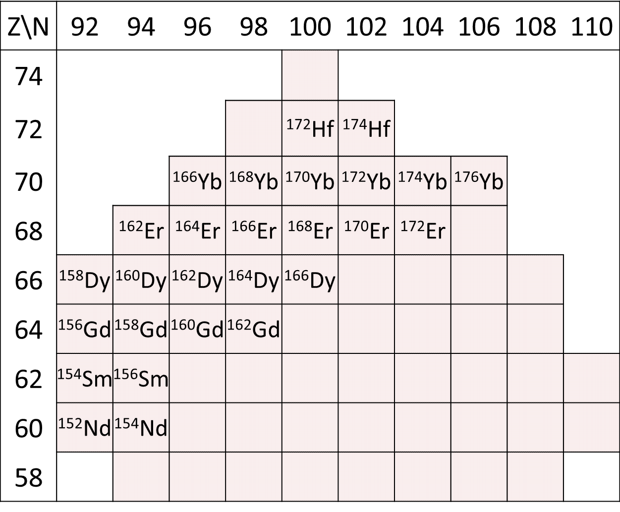
Figure 1: (Color online) Rare-earth region of the isotopic chart. Shaded area shows nuclei with deformation $\beta\geq 0.3$ in HFB calculations with SkM^∗ (unpublished, see Ref. Stoitsov et al. (2003) for SLy4 which gives a similar result). We calculate energies and transition probabilities of $\gamma$-vibrational states for all nuclei whose isotopic symbols appear in the figure. Squares without symbols correspond to nuclei for which experimental data on $\gamma$ vibrations are not in Ref. nnd .

Our procedure has two steps: a Hartree-Fock-Bogoliubov (HFB) calculation with the Vanderbilt HFB code Blazkiewicz et al. (2005), and a QRPA calculation that uses the results of the HFB run. Both steps use B splines Boor (1978); Nürnberger (1989); Schumaker (2007) to represent wave functions on a 42 by 42 cylindrical mesh with $0\leq z,\rho\leq 20$ fm. We use box boundary conditions to discretize the continuum, and introduce a quasiparticle cutoff energy $E_{\textrm{cut}}$ of 60 MeV or 200 MeV in the HFB calculation to limit the set of quasiparticle wave functions that determine the density and the pairing tensor. The two cutoffs require different pairing strengths, which we adjust via the three-point formula Bohr and Mottelson (1969) so as to reproduce the pairing gaps of ¹⁷²Yb (obtained from experimental masses). In the other nuclei, this procedure usually reproduces overall pairing gaps to within $\pm$150 keV. We restrict the $z$-component of the angular momentum of the wave functions to be less than or equal to 19/2 $\hbar$.

Next we transform the quasiparticle wave functions to the canonical-basis and introduce two cutoff occupation probabilities $(v^{\textrm{cut}}_{\textrm{pair}})^{2}$ and $(v^{\textrm{cut}}_{\textrm{ph}})^{2}$, used also in our prior work Terasaki et al. (2005, 2008); Terasaki and Engel (2010), to truncate the two-canonical-quasiparticle basis in which we construct the QRPA Hamiltonian matrix. We take $((v^{\textrm{cut}}_{\textrm{pair}})^{2},((v^{\textrm{cut}}_{\textrm{ph}})^{2})=(10^{-4},10^{-8})$ for $E_{\textrm{cut}}=60$ MeV, and $(10^{-3},10^{-6})$ for $E_{\textrm{cut}}=200$ MeV in the $\gamma$-vibration calculation with SkM^∗. Those values make the dimension of the two-canonical-quasiparticle basis about 22000 in ¹⁷²Yb, a number that is large enough to yield a convergent result. In the other rare-earth nuclei, the dimension ranges from 19000 to 28000.

Spurious states associated with particle-number conservation make the necessary space much larger for “$\beta$-vibrations.” There we use $((v^{\textrm{cut}}_{\textrm{pair}})^{2},((v^{\textrm{cut}}_{\textrm{ph}})^{2})=(10^{-4},10^{-6})$ with $E_{\textrm{cut}}$ = 200 MeV, values with which the dimension of the two-canonical-quasiparticle space is 60000 to 75000. Even with this large dimension, however, the spurious state does not separate perfectly and we present results only for cases in which the separation is good.

Deriving the QRPA equations for an axially-symmetric system is tedious but not difficult and can be done by starting from the general equations in, e.g., Ref. Terasaki et al. (2005). In the appendix, therefore, we display only our representation of the Coulomb-direct matrix elements. These require more numerical effort than matrix elements of a $\delta$-interaction, and so benefit more from a computationally efficient procedure.

III $\bm{\gamma}$-vibrations

III.1 Energies and transition strengths

Figure 2: (Color online) Energies of $\gamma$-vibrational states from a) experiment nnd , b) SkM^∗, c) SLy4, and d) Delaroche et al. Delaroche et al. (2010).

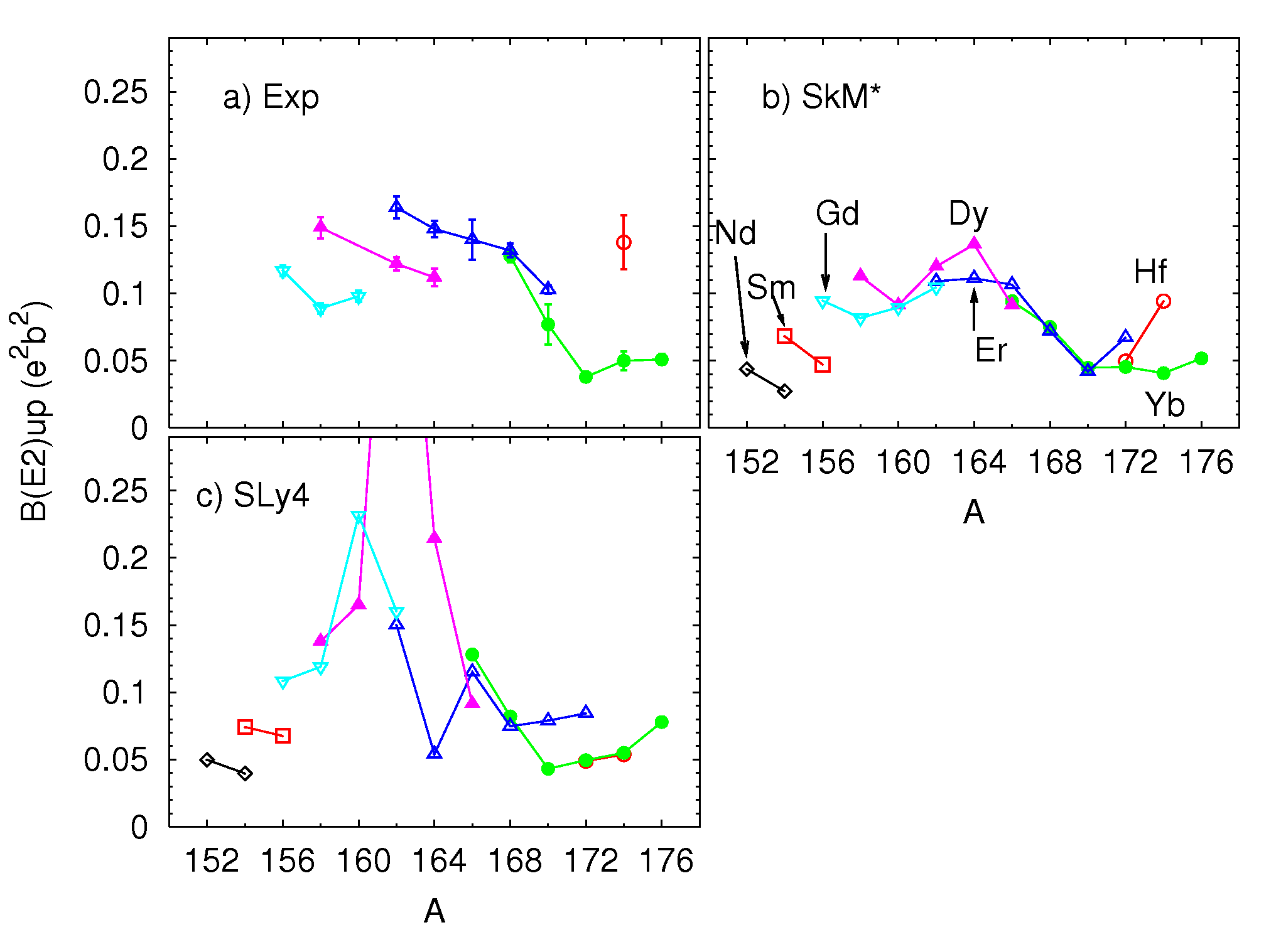
Figure 3: (Color online) $B(E2;0^{+}_{\textrm{gs}}\rightarrow 2^{+}_{\gamma})$ corresponding to Fig. 2. The value for ¹⁶²Dy in c) is 0.562 $e^{2}\textrm{b}^{2}$. This figure has no panel d) because the results from the calculation of Delaroche et al. Delaroche et al. (2010) are not published. We include only those experimental data that are labeled $\gamma$-vibrations in Ref. nnd . The symbols for particular isotopic chains are the same in each panel.

Figure 2 shows measured $\gamma$-vibration energies alongside the results of our two QRPA calculations and a collective-model calculation (with parameters determined from the Gogny energy functional) by Delaroche et al. Delaroche et al. (2010). In all the plots the minimum energy occurs around $A$=162. The minimum in the Dy and Er isotopes is at $N=98$, both in the data and the SkM^∗. The Yb isotopes are particularly well reproduced by the SkM^∗ calculation. But the QRPA calculations show a stronger $A$-dependence than the data, with the SLy4 results showing the strongest dependence. And overall, neither of the QRPA calculations is as good as that of Ref. Delaroche et al. (2010).

Figure 3 shows $E2$ transition strengths $B(E2;0^{+}_{\textrm{gs}}\rightarrow 2^{+}_{\gamma})$, hereafter denoted $B(E2)\!\!\uparrow$, for the same isotopes. Overall, the calculations reproduce the data reasonably well, except in ¹⁶²Dy with SLy4, and again are particularly good in the Yb isotopes. As before, SkM^∗ is noticeably better than SLy4. The energies and $B(E2)\!\!\uparrow$’s in our calculations are anticorrelated in general, a feature expected of harmonic vibrations. On the other hand, the experimental $B(E2)\!\!\uparrow$’s in Er decrease monotonically with $A$, even though the dependence of the energy is slightly parabolic.

To characterize the performance of the two functionals statistically, we introduce, following Refs. Terasaki et al. (2008); Bertsch et al. (2007) the measures

$$R_{E}=\ln\left(E_{\textrm{cal}}/E_{\textrm{exp}}\right)$$ (1)

and

$$R_{Q}=\ln\sqrt{B(E2)\!\!\uparrow_{\textrm{cal}}/B(E2)\!\!\uparrow_{\textrm{exp}}}\,,$$ (2)

where $E_{\textrm{cal}}$ and $E_{\textrm{exp}}$ are the calculated and experimental energies of the $\gamma$-vibrational state. The results are in Tab. 1. SLy4 actually does better than SkM^∗ in the averages, but gives much larger dispersions.

Table 1: Average of $R_{E}$ ($\bar{R}_{E}$), dispersion of $R_{E}$ ($\sigma_{E}$), and the same for $R_{Q}$.

	$\bar{R}_{E}$	$\sigma_{E}$	$\bar{R}_{Q}$	$\sigma_{Q}$
SkM∗	0.28	0.18	$-$0.13	0.14
SLy4	0.20	0.50	$-$0.004	0.31

Table 2 shows the statistical measures for the spherical nuclei treated in Ref. Terasaki et al. (2008) and for the subset of those nuclei that exhibit “low softness.” (Some of the other nuclei in Ref. Terasaki et al. (2008) are transitional.) There are far more nuclei in the spherical data set than in the deformed rare-earth set, so it is hard to make a precise comparison of performance. But deformation does not appear to affect it significantly.

Table 2: Statistical measures for the spherical nuclei and for the subset with low softness from Ref. Terasaki et al. (2008). $R_{Q}$ and $\sigma_{Q}$ were not calculated separately for the low-softness nuclei in that paper because of a lack of $E2$ data.

		$\bar{R}_{E}$	$\sigma_{E}$	$\bar{R}_{Q}$	$\sigma_{Q}$
All	SkM∗	0.11	0.44	-0.29	0.53
	SLy4	0.33	0.51	-0.32	0.42
Low Softness	SkM∗	0.27	0.35	—	—
	SLy4	0.47	0.48	—	—

III.2 $\bm{N}$- and $\bm{Z}$-dependence

Our calculations show a stronger dependence on $N$ than do the data in most isotopic chains, behavior that may be due to insufficient configuration mixing in our calculations. Figure 4 shows the $N$-dependence of the calculated $\gamma$-vibrational energy, the two-quasiparticle energy $E_{\textrm{2qp}}^{\textrm{Xn}}$ of the component, in the quasiparticle basis, with the largest neutron forward amplitude, and the absolute value of the backward amplitude $|Y_{\textrm{Xn}}|$ of the same component, all for SkM^∗. (We transformed amplitudes from the canonical-quasiparticle basis to do this analysis.) For $N\leq$ 100, The $\gamma$-vibrational energy is positively correlated with $E_{\textrm{2qp}}^{\textrm{Xn}}$, and anticorrelated with $|Y_{\textrm{Xn}}|$, indicating a connection between the $N$-dependence of those solutions and a particular two-quasiparticle state. The downward shift of about 1 MeV between the two-quasiparticle energy and the full QRPA energy, seen in panels a) and b), then characterizes the effect of the residual interaction. Fig. 5 shows all the same phenomena in the $Z$ dependence of our results, except in the energies of the $N=102$ isotones.

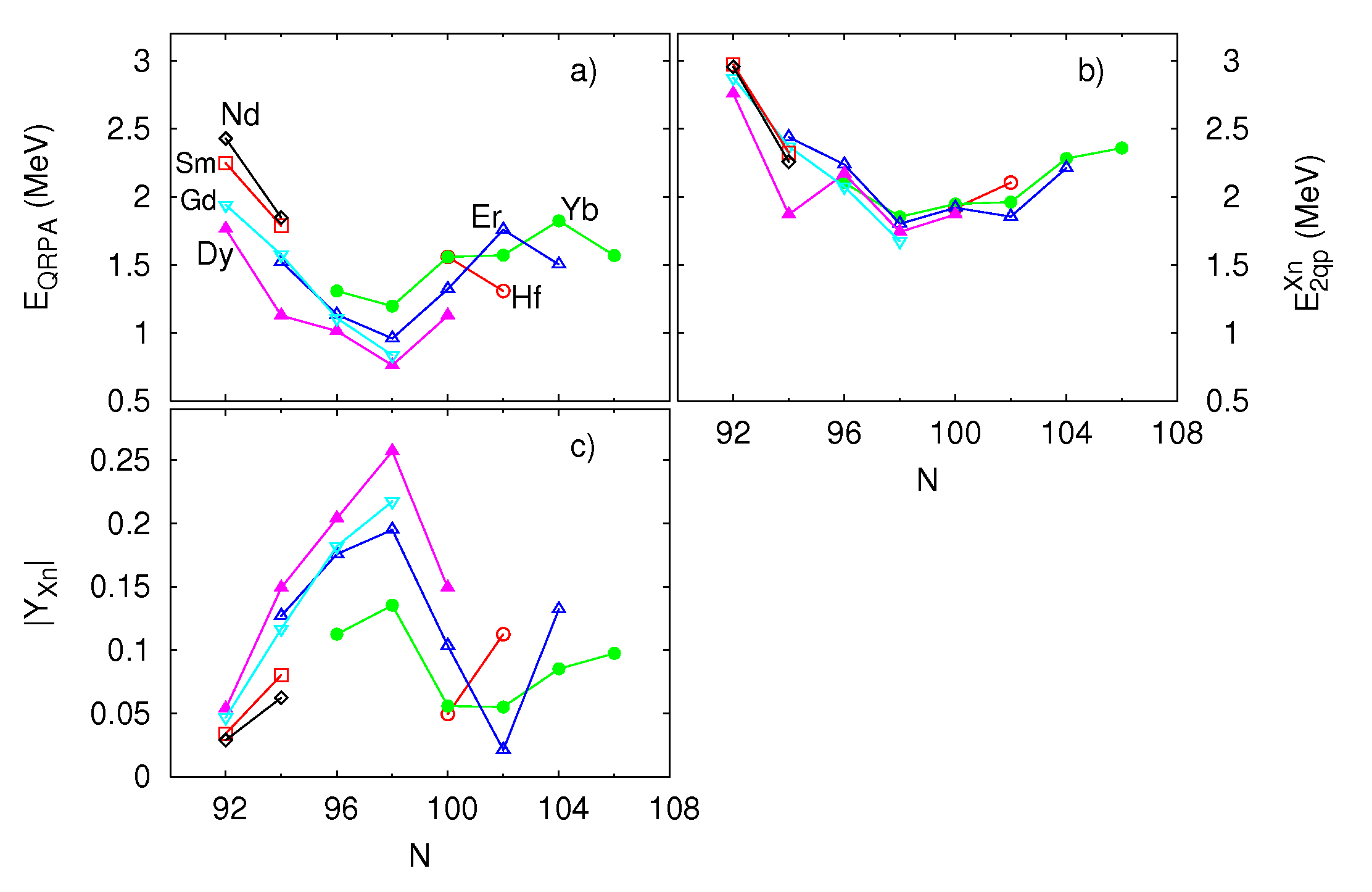
Figure 4: (Color online) For the functional SkM^∗, a) Calculated $\gamma$-vibrational energy, b) two-quasiparticle energy $E_{\textrm{2qp}}^{\textrm{Xn}}$ of the component with the largest neutron forward amplitude, and c) absolute value $|Y_{\textrm{Xn}}|$ of the backward amplitude of the same component, all as functions of neutron number $N$.

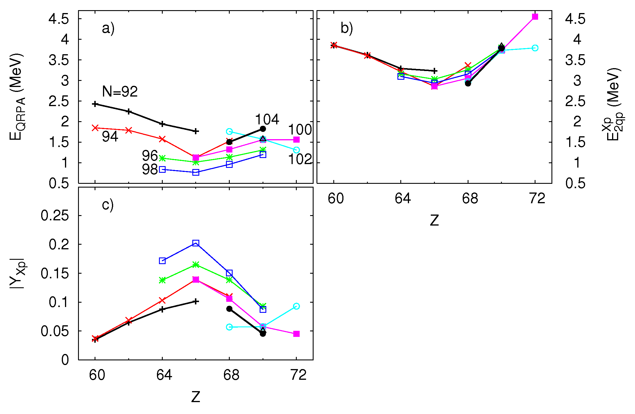
Figure 5: (Color online) The same panels as Fig. 4 but for protons rather than neutrons. The connected points are isotones, and the same symbol indicates a given isotone in each panel. $E_{\textrm{2qp}}^{\textrm{Xp}}$ and $|Y_{\textrm{Xp}}|$ now refer to the proton components.

Figure 6 shows the absolute values of the nine largest neutron forward amplitudes in three Dy isotopes around ¹⁶⁴Dy, which is the one with the lowest phonon energy. Clearly the two largest components are far more important than the rest. And though we don’t show it, a similar curve characterizes the protons. From all this, we conclude that the two-quasiparticle state with the largest neutron forward amplitudes plays a significant role in the $N$-dependences of the QRPA solutions, and that the same statement is true of proton forward amplitudes and $Z$ dependence. (The second largest components are potentially also important.) The weaker $N$- and $Z$-dependence in the data suggests that we exaggerate the importance of those particular two-quasiparticle states, perhaps by underestimating configuration mixing. It is quite possible that a better solution requires many-body correlations beyond the QRPA.

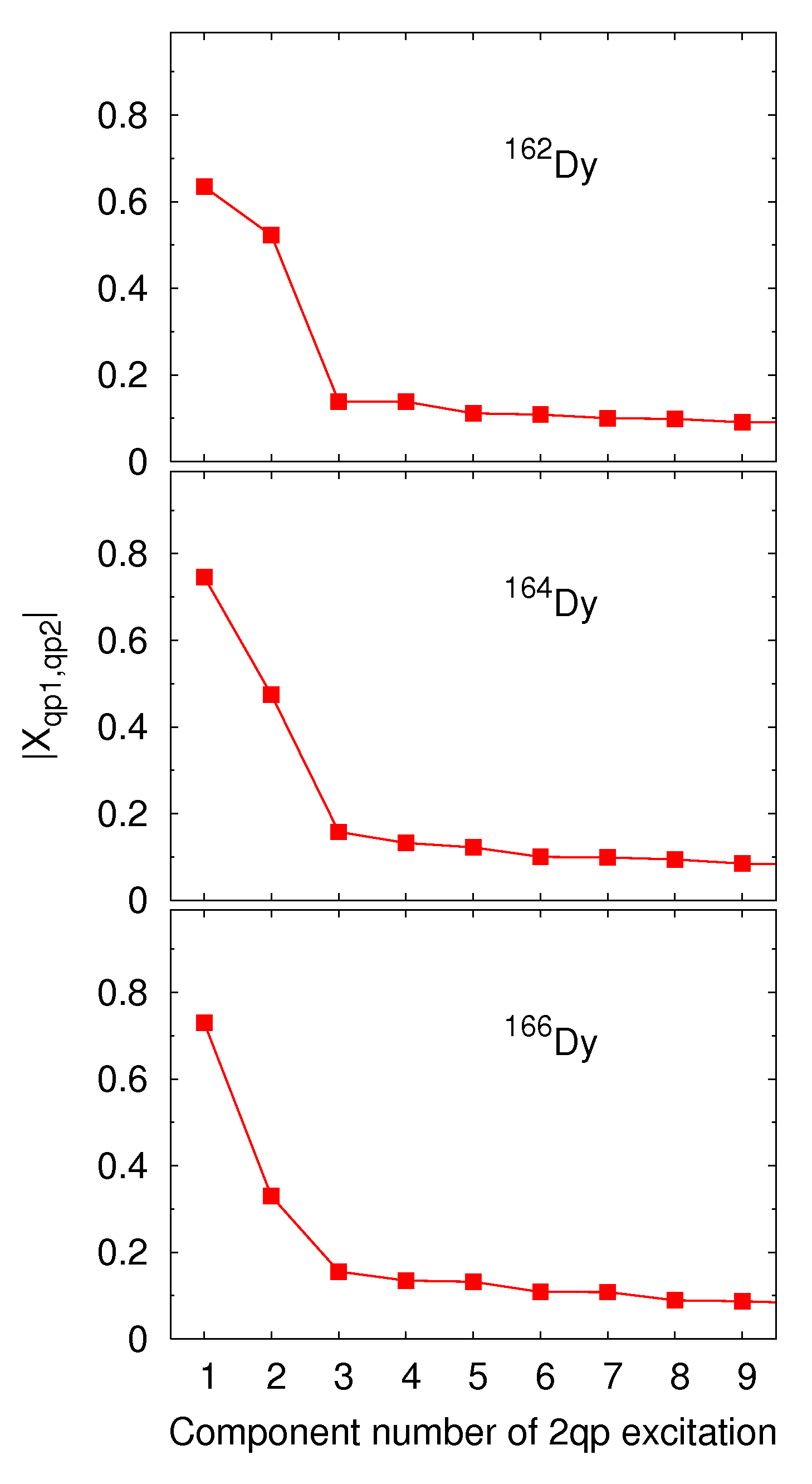
Figure 6: (Color online) Absolute values of the nine largest neutron forward amplitudes in ^162-166Dy. The integer on the $x$-axis labels the two-quasiparticle components.

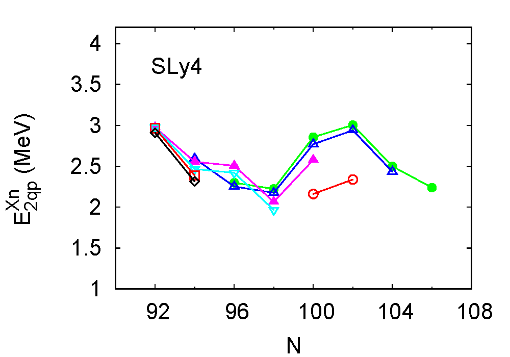
Figure 7: (Color online) $E^{\textrm{Xn}}_{\textrm{2qp}}$ produced by SLy4. The symbols correspond to those of Fig. 4.

Figure 7 shows $E^{\textrm{Xn}}_{\textrm{2qp}}$ for the SLy4 calculation. Interestingly, the range of the $E^{\textrm{Xn}}_{\textrm{2qp}}$ is close to that produced by SkM^∗, as one can see by comparing with panel b) of Fig. 4. We conclude that the effects of the residual interaction on $A$ dependence are quite different in the two calculations, leading to the noticeable differences in Fig. 2.

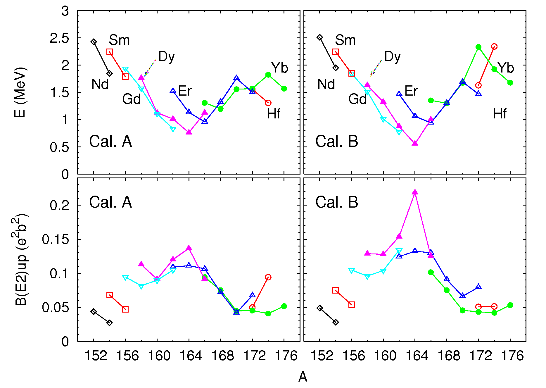
Figure 8: (Color online) Results of two calculations with different values for $E_{\textrm{cut}}$ and the pairing strength $G_{q}$, where $q$=p (proton) or n (neutron). Calculation A (left) uses ($E_{\textrm{cut}}$, $G_{\textrm{n}}$, $G_{\textrm{p}}$) = (60 MeV, 218.521 MeV fm³, 176.364 MeV fm³), and calculation B (right) uses (200 MeV, 168.384 MeV fm³, 143.996 MeV fm³). The SkM^∗-based results discussed in prior sections were obtained from Calculation A.

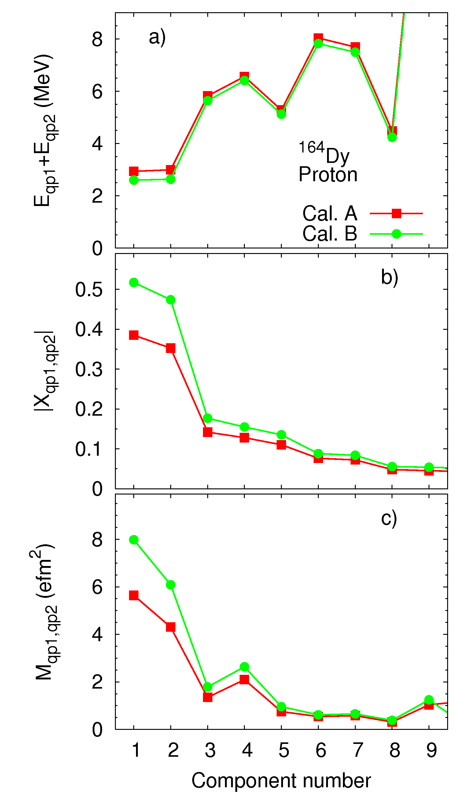
Figure 9: (Color online) Analysis of two-proton-quasiparticle configurations in the $\gamma$-vibrational state of ¹⁶⁴Dy, with SkM^∗: a) Two-quasiparticle energies, b) absolute values of the forward amplitude, c) contribution to the transition matrix element. The $x$ axis is the same as in Fig. 6. The pairing parameters characterizing calculations A and B are given in the caption of Fig. 8.

III.3 $\bm{\delta}$-pairing functional

Low-energy quasiparticle states are obviously affected by the choice of pairing functional, and the volume pairing we use can be varied without worsening its ability to reproduce pairing gaps. The reason is that the $\delta$-function interaction is singular in the pairing channel and so must be regularized (see, e. g. Ref. Bulgac and Yu (2002)). Here we do so by cutting off the single-quasiparticle spectrum. This procedure makes the strength of the interaction depend on the cutoff as well as on the experimental pairing gaps to which it is fit. To illustrate the effect of the cutoff on $\gamma$ vibrations, we show in Fig. 8 the results of calculations with the two different cutoffs $E_{\textrm{cut}}$ mentioned in Sec. II. The two cutoffs require different pairing strengths $G_{q}$ (for the values, see the caption) to ensure similar predictions for pairing gaps. We refer to the two calculations as A and B, with A having the smaller $E_{\textrm{cut}}$, and therefore the larger pairing strength.

The differences in the results are mostly minor, but the $B(E2)\!\!\uparrow$ in ¹⁶⁴Dy, the energy and $B(E2)\!\!\uparrow$ in ¹⁷⁴Hf, and the energy in ¹⁷²Yb are all quite different. We account for the differences in ¹⁶⁴Dy by referring to Fig. 9. Since calculation A uses a larger pairing strength, it produces higher energies for low-lying quasiparticles than does calculation B. In the separable approximation Nesterenko et al. (2006); Severyukhin et al. (2008), the forward QRPA amplitudes can be written as

$$X_{\textrm{ qp1,qp2}}\propto 1/(E_{\textrm{qp1}}+E_{\textrm{qp2}}-E_{\gamma})\,,$$ (3)

where qp1 and qp2 denote quasiparticle states, and $E_{\gamma}$ is the energy of the $\gamma$-vibrational state. Using Eq. (3) and the values read from the figures, one can estimate the ratio of the forward amplitudes of the largest two-quasiprarticle component in calculations A and B. The result, under the assumption that the interaction matrix elements are the same in the two calculations, is

$$\bigg{|}\frac{X_{\textrm{qp1,qp2}}^{A}}{X_{\textrm{qp1,qp2}}^{B}}\bigg{|}\simeq 0.9\,.$$ (4)

Panel b of Fig. 9 shows that the exact ratio is 0.8, so that half the difference between the two calculations can be explained by considering only the quasiparticle energies. This analysis implies that the QRPA solution is sensitive to the energies of important quasiparticle states, and thus to the pairing functional, when those energies are small. One can take advantage of this to fix the cutoff energy as well as the pairing strength by fitting to properties that depend sensitvely on low-energy quasiparticle states. Our calculation shows, for example, that $E_{\textrm{cut}}=60$ MeV is better than 200 MeV.

The differences between calculations A and B in ¹⁷²Yb and ¹⁷⁴Hf are more complicated (the corresponding two-quasiparticle components do not have the same order as Fig. 9), and we could not find a simple explanation for them. And changes in the pairing cutoff are clearly not enough to fix the problem with $N$- and $Z$-dependence in the QRPA.

III.4 Comparison with older calculations of $\bm{\gamma}$-vibrational states

Early work on vibrations in rare-earth nuclei often made use of the pairing-plus-QQ (quadrupole-quadrupole) Hamiltonian, both in the (Q)RPA Marshalek and Rasmussen (1963); Bès et al. (1965); Zielińska-Pfabe (1971); Hamamoto (1983); Matsuo and Matsuyanagi (1987) and in approximations that went beyond the QRPA order, e. g. Kishimoto and Tamura (1976); Soloviev and Shirikova (1989); Soloviev and Sushkov (1993). Single-particle energies were usually obtained from the Nilsson potential, with slight shifts to improve phenomenology, and the strength of the QQ interactions was modified slightly from the self-consistent value so as to reproduce the energies of the $\gamma$-vibrational states. The adjustment to energies means that $B(E2)\!\!\uparrow$’s are an important test of the model’s predictive power.

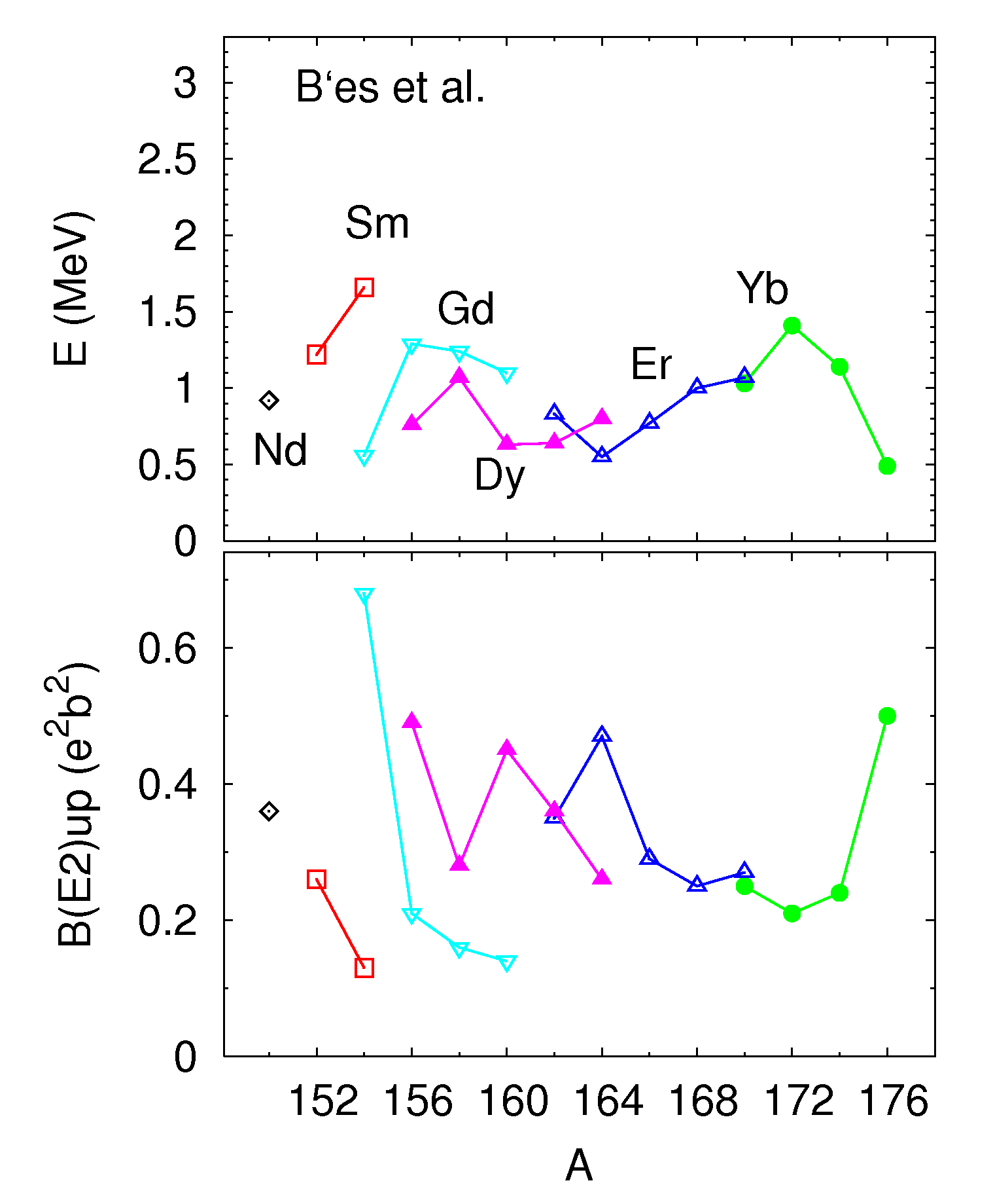
Figure 10: (Color online) Energy (upper panel), and $B(E2)\!\!\uparrow$ (lower panel) of $\gamma$-vibrational states in calculations by D. R. Bès et al. Bès et al. (1965)

Figure 10 shows the energies and $B(E2)\!\!\uparrow$ from Ref. Bès et al. (1965). Their energies were perhaps not quite as good overall as ours, but also did not exhibit the sharp minimum we get around $A\sim$ 164. The authors themselves stated that no single interaction strength reproduces the energies of all nuclei calculated. Their $B(E2)\!\!\uparrow$’s are too large by a factor of two or more, a deficiency that was pointed out again in Refs. Marshalek and Rasmussen (1963); Hamamoto (1983). Marshalek et al. Marshalek and Rasmussen (1963) listed approximations that might cause problems in predicted $B(E2)\!\!\uparrow$’s. Since we do better in that observable, we believe that the cause is in fact the interaction.

Rare-earth $\gamma$ vibrations have also been addressed in other models. Reference Kishimoto and Tamura (1976), using the boson-expansion method, obtained $B(E2)\!\!\uparrow$ = 0.130 $e^{2}$b² in ¹⁵⁴Sm, a value somewhat larger than ours. Soloviev et al. Soloviev and Shirikova (1989); Soloviev and Sushkov (1993) used the quasiparticle-phonon nuclear model, which includes two-phonon couplings, and obtained $B(E2)\!\!\uparrow$ = 0.127 $e^{2}$b² (¹⁶⁸Er), 0.042 $e^{2}$b² (¹⁷²Yb), and 0.122 $e^{2}$b² (¹⁷⁸Hf). Those transition probabilities are close to the experimental data (0.116 $e^{2}$b²in ¹⁷⁸Hf Soloviev and Shirikova (1989)), and the fit of the interaction meant that energies were also reproduced well. See also Ref. Matsuo and Matsuyanagi (1987) which used a modified QQ and an effective three-body interactions.

Explicitly collective models have also been used. Kumar Kumar (1967) obtained an energy of 1.438 MeV (close to the measured value) and a $B(E2)\!\!\uparrow$ of 0.163 $e^{2}$b² for the $\gamma$-vibrational state of ¹⁵⁴Sm by solving the Schrödinger equation in collective quadrupole degrees of freedom (Bohr and Mottelson’s collective model) with the Myers-Swiatechi potential. García-Ramos et al. García-Ramos et al. (2003) used the interacting boson model (IBM) to obtain low-energy states in about 20 even-even rare-earth nuclei, eight of which are discussed here. For each isotopic chain they determined the parameters of the IBM Hamiltonian by approximately reproducing the measured excitation energies for $J^{\pi}$ = 2${}^{+}_{1}$, 4${}^{+}_{1}$, 6${}^{+}_{1}$, 8${}^{+}_{1}$, 0${}^{+}_{2}$, 2${}^{+}_{3}$, 4${}^{+}_{3}$, 2${}^{+}_{2}$, 3${}^{+}_{1}$, and 4${}^{+}_{2}$ states, and determined the boson effective charge by reproducing several measured $B(E2)$’s. With regard to the $\gamma$-vibrational $B(E2)\!\!\uparrow$’s of the eight nuclei computed here, they reproduced those of ^158,160Gd well but overestimated others. See also Ref. Warner and Casten (1983), which presented another set of IBM calculations.

IV $\bm{\beta}$-vibrations

In Tab. 3 we show calculated and measured energies and $B(E2)\!\!\uparrow$’s, with SkM^∗, for “$\beta$-vibrational” states. As mentioned earlier, the $K^{\pi}=0^{+}$ channel contains a spurious state, and we display only those “$\beta$-vibrations” that are clearly uncontaminated by spurious motion (see the last column of the table).

Table 3: Properties of “$\beta$-vibrational” states in four nuclei. $E_{\textrm{cal}}^{\beta}$ and $E_{\textrm{exp}}^{\beta}$ are the calculated (with SkM^∗) and experimental energies. $B(E2)\!\!\uparrow_{\textrm{cal}}^{\beta}$ and $B(E2)\!\!\uparrow_{\textrm{exp}}^{\beta}$ are the corresponding reduced upward transition probabilities. The “Ratio of $S_{N}$” is the ratio of the (spurious) strength associated with the particle-number operator Terasaki and Engel (2010) for the “$\beta$-vibrational” state to that for the spurious state (average of proton and neutron).

Nucleus	$E_{\textrm{cal}}^{\beta}$	$E_{\textrm{exp}}^{\beta}$	$B(E2)\!\!\uparrow_{\textrm{cal}}^{\beta}$	$B(E2)\!\!\uparrow_{\textrm{exp}}^{\beta}$	Ratio of $S_{N}$
	(MeV)	(MeV)	$(e^{2}\textrm{b}^{2})$	$(e^{2}\textrm{b}^{2})$
166Yb	1.802	1.043	0.0398		0.004
168Yb	2.039	1.155	0.0343		0.012
172Yb	1.605	1.117	0.0049	0.0081(17)	0.054
170Er	1.596	0.960	0.0030	0.0079(9)	0.054

We obtained these results with calculation B (see above), the large cutoff in which should lead to a more accurate treatment of the spurious state, though contamination in nuclei not shown in the table indicates that a finer mesh is necessary with a large cutoff. In our previous paper Terasaki and Engel (2010), which used $E_{\textrm{cut}}$ = 60 MeV, $E_{\textrm{cal}}^{\beta}$ and $B(E2)\!\!\uparrow_{\textrm{cal}}^{\beta}$ were 1.390 MeV and 1.117 $e^{2}\textrm{b}^{2}$ in ¹⁷²Yb; our new energy is thus 15% larger. Compared to the $\gamma$-vibrational states, overall we apparently overestimate energies and underestimate $B(E2)\!\!\uparrow$’s, and do not do as good a job as with $\gamma$-vibrational sates. Reference Garrett (2001) points out that “$\beta$-vibrational” states are not purely vibrational, and in many cases are better interpreted as the second member of the $K^{\pi}$=0⁺ yrare rotational band. The QRPA cannot describe rotational bands and so the discrepancy between our results and experiment is not totally surprising.

V Conclusion

We have used the QRPA with the Skyrme functionals SkM^∗ and SLy4 and volume-$\delta$-pairing to calculate the energies and $B(E2)\!\!\uparrow$’s of $\gamma$-vibrational states in well-deformed even-even rare-earth nuclei. SkM^∗ proves to be the better functional. The range of calculated values overlaps well with that of the experimental data. Since the QRPA energies are appreciably different from their unperturbed counterparts, that counts as a success for the residual interaction; the vibrational states discussed here are not taken into account at all in determining energy functionals. In detail, however, the calculations are far from perfect, and their $N$- and $Z$- dependence suggest the importance of many-body correlations that are not included in the QRPA. And our representation of “$\beta$-vibrational” states turns to be worse than that of $\gamma$ vibrations, probably because “$\beta$ vibrations” are often not really vibrations.

We also suggested that the cutoff associated with volume pairing can be fixed along with the pairing strength by examining properties that are sensitive to the structure of low-lying quasiparticles.

Our calculation is better overall than the works of half a century ago. The aims of the pairing-plus-QQ model are much more limited than those of nuclear DFT; the mean field arising from pairing-plus-QQ is an infinitely deep well, and so the model cannot make predictions for binding energies or for excitation energies near the drip line (where the underlying Nilsson single-particle potential is not appropriate). Despite the increasing sophistication of the many-body methods that have been applied together with the pairng-plus-QQ model, a more general framework such as DFT appears necessary for the unified description of heavy nuclei.

Finally, we have shown that in this era of supercomputing a scalable code makes systematic and fully self-consistent Skyrme-QRPA studies possible. We expect, as a result, that excited states will play an increasing role in the determination of nuclear density functionals.

*

Appendix A Coulomb-direct matrix elements

The computation of the direct two-body matrix elements of the Coulomb interaction consumes a lot of computing time. In this appendix we present our implementation of that computation.

The Coulomb interaction is

$$V_{\textrm{C}}(\bm{r}_{1},\bm{r}_{2})=\frac{e^{2}}{\lvert\bm{r}_{1}-\bm{r}_{2}\rvert}\,.$$ (5)

We take advantage of axial symmetry to write the wave function as

$$X_{a}(\bm{r})=\frac{1}{\sqrt{2\pi}}\sum_{\sigma=\pm{1/2}}{\cal F}_{a}(\sigma;z,\rho)e^{i(j^{z}_{a}-\sigma)\phi}|\sigma\rangle~{},$$ (6)

The label $a$ stands for $(q\pi j_{z}i)$, i. e. particle type, parity, angular-momentum $z$-component, and an additional label $i$ to fully specify the state. The position $\bm{r}$ is represented in cylindrical coordinates, and the label $\sigma=\pm 1/2$ is the $z$-component of the spin. The function ${\cal F}_{a}(\sigma;z,\rho)$ is treated numerically. The set $\{X_{a}(\bm{r})\}$ can refer to any single-particle basis (or components of quasiparticle basis states, in which case another label to distinguish upper from lower is necessary) with axial and parity symmetries. In our calculations we use the canonical single-particle basis.

With the help of a few well-known formulae from Appendix B of Ref. Messiah (1961), one can obtain the expansion

$$\frac{1}{|\bm{r}_{1}-\bm{r}_{2}|} =\sum_{l=0}^{\infty}\frac{(\sqrt{\rho_{<}^{2}+z_{<}^{2}})^{l}}{(\sqrt{\rho_{>}^{2}+z_{>}^{2}})^{l+1}}\sum_{m=-l}^{l}\frac{(l-m)!}{(l+m)!}$$ (7)

$$P_{lm}\bigglb(\frac{z_{1}}{\sqrt{\rho_{1}^{2}+z_{1}^{2}}}\biggrb)P_{lm}\bigglb(\frac{z_{2}}{\sqrt{\rho_{2}^{2}+z_{2}^{2}}}\biggrb)$$

$$e^{im(\phi_{2}-\phi_{1})}~{},$$

where

$$\begin{array}[]{l}\rho_{<}^{2}+z_{<}^{2}=\rho_{1}^{2}+z_{1}^{2}\\ \rho_{>}^{2}+z_{>}^{2}=\rho_{2}^{2}+z_{2}^{2}\end{array}\Bigr{\}}~{},~{}\textrm{if}~{}\rho_{2}^{2}+z_{2}^{2}>\rho_{1}^{2}+z_{1}^{2}~{},$$ (10)

$$\begin{array}[]{l}\rho_{<}^{2}+z_{<}^{2}=\rho_{2}^{2}+z_{2}^{2}\\ \rho_{>}^{2}+z_{>}^{2}=\rho_{1}^{2}+z_{1}^{2}\end{array}\Bigr{\}}~{},~{}\textrm{if}~{}\rho_{2}^{2}+z_{2}^{2}<\rho_{1}^{2}+z_{1}^{2}~{},$$ (13)

and the $P_{lm}$ are associated Legendre polynomials Messiah (1961). By using Eqs. (5)$-$(13), one can then write the matrix element of the Coulomb-direct interaction as

$$V^{\textrm{C}}_{ab,cd} = \int d^{3}\bm{r}_{1}\int d^{3}\bm{r}_{2}X_{a}^{\dagger}(\bm{r}_{1})X_{b}^{\dagger}(\bm{r}_{2})V_{\textrm{C}}(\bm{r}_{1},\bm{r}_{2})X_{c}(\bm{r}_{1})X_{d}(\bm{r}_{2})$$ (14)

$$= e^{2}\sum_{\sigma_{a},\sigma_{b}}\sum_{l=0}^{\infty}\sum_{m=-l}^{l}\delta_{-j^{z}_{a}-m+j^{z}_{c},0}\delta_{-j^{z}_{b}+m+j^{z}_{d},0}\int_{-\infty}^{\infty}dz_{1}\int_{0}^{\infty}d\rho_{1}\rho_{1}\int_{-\infty}^{\infty}dz_{2}\int_{0}^{\infty}d\rho_{2}\rho_{2}{\cal F}_{a}(\sigma_{a};z_{1},\rho_{1})$$

$$P_{lm}\bigglb(\frac{z_{1}}{\sqrt{\rho_{1}^{2}+z_{1}^{2}}}\biggrb){\cal F}_{c}(\sigma_{a};z_{1},\rho_{1}){\cal F}_{b}(\sigma_{b};z_{2},\rho_{2})P_{lm}\bigglb(\frac{z_{2}}{\sqrt{\rho_{2}^{2}+z_{2}^{2}}}\biggrb){\cal F}_{d}(\sigma_{b};z_{2},\rho_{2})\frac{\biglb(\sqrt{\rho_{<}^{2}+z_{<}^{2}}\bigrb)^{l}}{\biglb(\sqrt{\rho_{>}^{2}+z_{>}^{2}}\bigrb)^{l+1}}$$

$$\frac{(l-m)!}{(l+m)!}~{}.$$

Changing variables to

$$(z,R=\sqrt{\rho^{2}+z^{2}})~{},$$ (15)

and noting that

$${\cal F}_{a}(\sigma_{a};-z,\rho)=(-)^{j^{z}_{a}-\sigma_{a}}\pi_{a}{\cal F}_{a}(\sigma_{a};z,\rho)~{},$$ (16)

$$P_{lm}(-x)=(-)^{l-m}P_{lm}(x)~{},$$ (17)

we arrive at

$$V^{\textrm{C}}_{ab,cd} = 4e^{2}\delta_{-j^{z}_{a}+j^{z}_{c},j^{z}_{b}-j^{z}_{d}}\delta_{\pi_{a}\pi_{c},\pi_{b}\pi_{d}}\sum_{\sigma_{a},\sigma_{b}}\sum_{l=\lvert-j^{z}_{a}+j^{z}_{c}\rvert}^{\infty}\delta_{\pi_{a}\pi_{c},(-)^{l}}\frac{(l-m)!}{(l+m)!}\bigglb\{\int_{0}^{\infty}dR_{1}\frac{{\cal T}_{1}(R_{1})}{R_{1}^{l-1}}\int_{0}^{R_{1}}dR_{2}R_{2}^{l+2}{\cal T}_{2}(R_{2})$$ (18)

$$+\int_{0}^{\infty}dR_{1}{\cal T}_{1}(R_{1})R_{1}^{l+2}\int_{R_{1}}^{\infty}dR_{2}\frac{{\cal T}_{2}(R_{2})}{R_{2}^{l-1}}\biggrb\}\biggrb\rvert_{m=-j^{z}_{a}+j^{z}_{c}}~{},$$

where

$${\cal T}_{1}(R_{1})=\frac{1}{R_{1}}\int_{0}^{R_{1}}dz_{1}{\cal F}_{a}\Biglb(\sigma_{a};z_{1},\sqrt{R_{1}^{2}-z_{1}^{2}}\Bigrb)P_{lm}\bigglb(\frac{z_{1}}{R_{1}}\biggrb){\cal F}_{c}\Biglb(\sigma_{a};z_{1},\sqrt{R_{1}^{2}-z_{1}^{2}}\Bigrb)~{},$$

$${\cal T}_{2}(R_{2})=\frac{1}{R_{2}}\int_{0}^{R_{2}}dz_{2}{\cal F}_{b}\Biglb(\sigma_{b};z_{2},\sqrt{R_{2}^{2}-z_{2}^{2}}\Bigrb)P_{lm}\bigglb(\frac{z_{2}}{R_{2}}\biggrb){\cal F}_{d}\Biglb(\sigma_{b};z_{2},\sqrt{R_{2}^{2}-z_{2}^{2}}\Bigrb)~{}.$$ (19)

Though it is not explicit in the notation, ${\cal T}_{1}(R_{1})$ depends on the labels $a$, $c$, $\sigma_{a}$, and $(l,m)$, and ${\cal T}_{2}(R_{2})$ on similar quantities.

Equations (18) and (19) are what we use, with minor modifications for hole states, in our code. We calculate ${\cal T}_{1}(R_{1})$ and ${\cal T}_{2}(R_{2})$ on a mesh and store them in arrays. Once this is finished, the time to calculate Eq. (18) is determined mainly by the nest structure of the two-fold integrals and the summation with respect to $l$. For a system with quadrupole deformation $\beta\sim$ 0.3 the number of terms necessary in the sum over $l$ (much fewer than 20 in practice, with only even or only odd $l$ contributing) is much smaller than the number of mesh points in the integration.

If an equidistant mesh is used for integrals in which an upper or lower bound is a variable, the computational effort to calculate the two-fold integrals in Eq. (18) is nearly the same as that of single integrals. Thus, we calculate the wave functions on a new mesh by interpolating between B-spline points, and then use Simpson’s rule with three times more mesh points than B-spline points to preserve accuracy (while still speeding up the integration). We have checked our procedure by using the two-body matrix elements that it produces to calculate the Coulomb-direct energy of the HFB ground state, which we then compared to the output of the HFB code.

References

- Pieper et al. (2004) S. C. Pieper, R. B. Wiringa, and J. Carlson, Phys. Rev. C 70, 054325 (2004).
- Pieper and Wiringa (2001) S. C. Pieper and R. B. Wiringa, Annu. Rev. Nucl. Part. Sci. 51, 53 (2001).
- Negoita et al. (2010) A. G. Negoita, J. P. Vary, and S. Stoica, J. Phys. G 37, 055109 (2010).
- Vary et al. (2009) J. P. Vary, S. Popescu, S. Stoica, and P. Navrátil, J. Phys. G 36, 085103 (2009).
- Hagen et al. (2007) G. Hagen, D. J. Dean, M. Hjorth-Jensen, T. Papenbrock, and A. Schwenk, Phys. Rev. C 76, 044305 (2007).
- Dean and Hjorth-Jensen (2004) D. Dean and M. Hjorth-Jensen, Phys. Rev. C 69, 054320 (2004).
- Dobaczewski (2010) J. Dobaczewski, e-print arXiv:nucl-th/1009.0899 (2010), to be published in J. of Phys. : Conference Series.
- Kortelainen et al. (2010) M. Kortelainen, T. Lesinski, J. Moré, W. Nazarewicz, J. Sarich, N. Schunck, M. V. Stoitsov, and S. Wild, Phys. Rev. C 82, 024313 (2010).
- Goriely and Khan (2002) S. Goriely and E. Khan, Nucl. Phys. A 706, 217 (2002).
- Terasaki and Engel (2010) J. Terasaki and J. Engel, Phys. Rev. C 82, 034326 (2010).
- Péru et al. (2011) S. Péru, G. Gosselin, M. Martini, M. Dupuis, S. Hilaire, and J.-C. Devaux, Phys. Rev. C 83, 014314 (2011).
- Yoshida and Nakatsukasa (2011) K. Yoshida and T. Nakatsukasa, Phys. Rev. C 83, 021304(R) (2011).
- Garrett (2001) P. E. Garrett, J. Phys. G 27, R1 (2001).
- Oshima et al. (1995) M. Oshima, T. Morikawa, Y. Hatsukawa, S. Ichikawa, N. Shinohara, M. Matsuo, H. Kusakari, N. Kobayashi, M. Sugawara, and T. Inamura, Phys. Rev. C 52, 3492 (1995).
- Sugawara et al. (1993) M. Sugawara, H. Kusakari, T. Morikawa, H. Inoue, Y. Yoshizawa, A. Virtanen, M. Piiparinen, and T. Horiguchi, Nucl. Phys. A 557, 653 (1993).
- Fahlander et al. (1992a) C. Fahlander, B. Varnestig, A. Bäcklin, L. E. Svensson, D. Disdier, L. Kraus, I. Linck, N. Schulz, and J. Pedersen, Nucl. Phys. A 541, 157 (1992a).
- Fahlander et al. (1992b) C. Fahlander, I. Thorslund, B. Varnestig, A. Bäcklin, L. E. Svensson, D. Disdier, L. Kraus, I. Linck, N. Schulz, J. Pedersen, et al., Nucl. Phys. A 537, 183 (1992b).
- Kotliński et al. (1990) B. Kotliński, D. Cline, A. Bäcklin, K. G. Helmer, A. E. Kavka, W. J. Kernan, E. G. Vogt, C. Y. Wu, R. M. Diamond, A. O. Macchiavelli, et al., Nucl. Phys. A 517, 365 (1990).
- Burke et al. (1988) D. G. Burke, G. Løvhøiden, and T. F. Thorsteinsen, Nucl. Phys. A 483, 221 (1988).
- Ichihara et al. (1987) T. Ichihara, H. Sakaguchi, M. Nakamura, M. Y. M. Ieiri, Y. Takeuchi, H. Togawa, T. Tsutsumi, and S. Kobayashi, Phys. Rev. C 36, 1754 (1987).
- Walker (1983) P. M. Walker, Phys. Scr. T5, 29 (1983).
- Ronningen et al. (1982) R. M. Ronningen, R. S. Grantham, J. H. Hamilton, R. B. Piercey, A. V. Ramayya, B. van Nooijen, H. Kawakami, W. Lourens, R. S. Lee, W. K. Dagenhart, et al., Phys. Rev. C 26, 97 (1982).
- Cresswell et al. (1981) J. R. Cresswell, P. D. Forsyth, D. G. E. Martin, and R. C. Morgan, J. Phys. G 7, 235 (1981).
- McGowan and Milner (1981) F. K. McGowan and W. T. Milner, Phys. Rev. C 23, 1926 (1981).
- Riedinger et al. (1979) L. L. Riedinger, E. G. Funk, J. W. Mihelich, G. S. Schilling, A. E. Rainis, and R. N. Oehlberg, Phys. Rev. C 20, 2170 (1979).
- McGowan et al. (1978) F. K. McGowan, W. T. Milner, R. L. Robinson, P. H. Stelson, and Z. W. Grabowski, Nucl. Phys. A 297, 51 (1978).
- Wollersheim and Th. W. Elze (1977) H. J. Wollersheim and Th. W. Elze, Z. Phys. A 280, 277 (1977).
- Ronningen et al. (1977) R. M. Ronningen, J. H. Hamilton, A. V. Ramayya, L. Varnell, G. Garcia-Bermudez, J. Lange, W. Lourens , L. L. Riedinger, R. L. Robinson, P. H. Stelson, et al., Phys. Rev. C 15, 1671 (1977).
- Reich et al. (1974) C. W. Reich, R. C. Greenwood, and R. A. Lokken, Nucl. Phys. A 228, 365 (1974).
- Baktash et al. (1974) C. Baktash, J. X. Saladin, J. O’Brien, I. Y. Lee, and J. E. Holden, Phys. Rev. C 10, 2265 (1974).
- Oehlberg et al. (1974) R. N. Oehlberg, L. L. Riedinger, A. E. Rainis, A. G. Schmidt, E. G. Funk, and J. W. Mihelich, Nucl. Phys. A 219, 543 (1974).
- Cardoso et al. (1973) M. H. Cardoso, P. F. A. Goudsmit, and J. Konijn, Nucl. Phys. A 205, 121 (1973).
- Bemis Jr. et al. (1973) C. E. Bemis Jr., P. H. Stelson, F. K. McGowan, W. T. Milner, J. L. C. Ford Jr., R. L. Robinson, and W. Tuttle, Phys. Rev. C 8, 1934 (1973).
- Domingos et al. (1972) J. M. Domingos, G. D. Symons, and A. C. Douglas, Nucl. Phys. A 180, 600 (1972).
- Gillin and Peek (1971) M. T. Gillin and N. F. Peek, Phys. Rev. 4, 1334 (1971).
- Charvet et al. (1971) A. Charvet, D. H. Phuoc, R. Duffait, A. Emsallem, and R. Chéry, J. de Physique 32, 359 (1971).
- Ejiri and Hageman (1971) H. Ejiri and G. B. Hageman, Nucl. Phys. A 161, 449 (1971).
- Grotdal et al. (1968) T. Grotdal, K. Nybø, T. Thorsteinsen, and B. Elbek, Nucl. Phys. A 110, 385 (1968).
- Veje et al. (1968) E. Veje, B. Elbek, B. Herskind, and M. C. Olesen, Nucl. Phys. A 109, 489 (1968).
- Bloch et al. (1967) R. Bloch, B. Elbek, and P. O. Tjøm, Nucl. Phys. A 91, 576 (1967).
- Yoshizawa et al. (1965) Y. Yoshizawa, B. Elbek, B. Herskind, and M. C. Olesen, Nucl. Phys. 73, 273 (1965).
- Nathan and Popov (1960) O. Nathan and V. I. Popov, Nucl. Phys. 21, 631 (1960).
- (43) [http://www.nndc.bnl.gov].
- Bartel et al. (1982) J. Bartel, P. Quentin, M. Brack, C. Guet, and H.-B. Håkansson, Nucl. Phys. A 386, 79 (1982).
- Chabanat et al. (1998) E. Chabanat, P. Bonche, P. Haensel, J. Meyer, and R. Schaeffer, Nucl. Phys. A 635, 231 (1998).
- Terasaki et al. (2005) J. Terasaki, J. Engel, M. Bender, J. Dobaczewski, W. Nazarewicz, and M. Stoitsov, Phys. Rev. C 71, 034310 (2005).
- Stoitsov et al. (2003) M. V. Stoitsov, J. Dobaczewski, W. Nazarewicz, S. Pittel, and D. J. Dean, Phys. Rev. C 68, 054312 (2003).
- Blazkiewicz et al. (2005) A. Blazkiewicz, V. E. Oberacker, A. S. Umar, and M. Stoitsov, Phys. Rev. C 71, 054321 (2005).
- Boor (1978) C. D. Boor, A Practical Guide to Splines (Springer, New York, 1978).
- Nürnberger (1989) G. Nürnberger, Approximation by Spline Functions (Springer, New York, 1989).
- Schumaker (2007) L. L. Schumaker, Spline Function : Basic Theory (Cambridge Univ. Press, Cambrige, 2007).
- Bohr and Mottelson (1969) A. Bohr and B. R. Mottelson, Nuclear Structure, vol. 1 (Benjamin, New York, 1969).
- Terasaki et al. (2008) J. Terasaki, J. Engel, and G. F. Bertsch, Phys. Rev. C 78, 044311 (2008).
- Delaroche et al. (2010) J.-P. Delaroche, M. Girod, J. Libert, H. Goutte, S. Hilaire, S. Péru, N. Pillet, and G. F. Bertsch, Phys. Rev. C 81, 014303 (2010).
- Bertsch et al. (2007) G. F. Bertsch, M. Girod, S. Hilaire, J.-P. Delaroche, H. Goutte, and S. Péru, Phys. Rev. Lett. 99, 032502 (2007).
- Bulgac and Yu (2002) A. Bulgac and Y. Yu, Phys. Rev. Lett. 88, 042504 (2002).
- Nesterenko et al. (2006) V. O. Nesterenko, W. Kleinig, J. Kvasil, P. Vesely, P.-G. Reinhard, and D. S. Dolci, Phys. Rev. C 74, 064306 (2006).
- Severyukhin et al. (2008) A. P. Severyukhin, V. V. Voronov, and N. V. Giai, Phys. Rev. C 77, 024322 (2008).
- Marshalek and Rasmussen (1963) E. R. Marshalek and J. O. Rasmussen, Nucl. Phys. 43, 438 (1963).
- Bès et al. (1965) D. R. Bès, P. Federman, E. Maqueda, and A. Zuker, Nucl. Phys. 65, 1 (1965).
- Zielińska-Pfabe (1971) M. Zielińska-Pfabe, Act. Phys. Pol. B 2, 207 (1971).
- Hamamoto (1983) I. Hamamoto, Suppl. Prog. Theor. Phys. 74 and 75, 157 (1983).
- Matsuo and Matsuyanagi (1987) M. Matsuo and K. Matsuyanagi, Prog. Theor. Phys 78, 591 (1987).
- Kishimoto and Tamura (1976) T. Kishimoto and T. Tamura, Nucl. Phys. A 270, 317 (1976).
- Soloviev and Shirikova (1989) V. G. Soloviev and N. Y. Shirikova, Z. Phys. A 334, 149 (1989).
- Soloviev and Sushkov (1993) V. G. Soloviev and A. V. Sushkov, Z. Phys. A 345, 155 (1993).
- Kumar (1967) K. Kumar, Nucl. Phys. A 92, 653 (1967).
- García-Ramos et al. (2003) J. E. García-Ramos, J. M. Arias, J. Barea, and A. Frank, Phys. Rev. C 68, 024307 (2003).
- Warner and Casten (1983) D. D. Warner and R. F. Casten, Phys. Rev. C 28, 1798 (1983).
- Messiah (1961) A. Messiah, Quantum Mechanics (North Holland, Amsterdam, 1961).