Cosmic ray propagators
in the fractional differential model of bounded anomalous diffusion

Abstract

Fractional differential approach to cosmic ray physics problems is discussed. A short review in this field is given, some results are represented, analyzed and criticized. A new model called the bounded anomalous diffusion model is offered. Its equation includes the fractional material derivative which allows to take into account the finite speed of cosmic rays particles.

1 Introduction

For a long time, cosmic rays (CR) propagation through the Galaxy have been described in frame of the normal diffusion theory, based on the equation

$$\left[\frac{\partial}{\partial t}-C\triangle\right]\psi(\mathbf{r},t)=\delta(t)\delta(\mathbf{r}),$$

where $C$ is the diffusion coefficient independent on frequency. This equation is derived under the assumption that fluctuations of interstellar magnetic fields, giving particle trajectories a specific (Brownian) character, are characterized by definite space sizes and look more homogeneous at large scales.

Rising attention to fractional calculus and its applications haven’t passed CR physics as well (see [Uchaikin(2008)]). An operator only symbolically different from the fractional derivative with respect to time, appeared (being unrecognized) in [Chuvilgin & Ptuskin (1993)]. The same derivative we meet in the equations derived by [Ragot & Kirk (1997), Balescu (1995)] (see also the reviewing part of recent work [Webb et al. (2006)]). Replacing the first time-derivative in the diffusion equation by its fractional analog reflects slowing-down of CR diffusion caused by magnetic traps (see [Dorman (1975)]). This kind of diffusion process was called subdiffusion.

At the same time, the turbulent (fractal) character of the interstellar magnetic field (see [Ruzmaikin et al. (1988), 8]) accelerates the diffusion. The turbulent diffusion (superdiffusion) was described by [Monin (1955)] by means of diffusion equation with fractional (2/3) power of Laplacian. [Saichev & Zaslavsky (1997)] and [Uchaikin & Zolotarev (1999)] combined both of these regimes (super- and subdiffusions) to one anomalous diffusion process, described by the space-time fractional equation

$$\left[{}_{0}\textsf{D}_{t}^{\beta}+C(-\triangle)^{\alpha/2}\right]\psi(\mathbf{r},t)=\frac{t^{-\beta}}{\Gamma(1-\beta)}\delta(\mathbf{r}),$$

Its solution depends on two parameters: fractional orders of the partial derivatives with respect to the coordinates ($\alpha\in(0,2]$) and time ($\beta\in(0,1]$). The characteristic features of this solution are the presence of heavy power-law tails (for $\alpha<2$) and the law of diffusion packet spreading $t^{\beta/\alpha}$. The family of distributions was named fractional stable distributions by [Kolokoltsov et al. (2000)], and investigated later in detail.

First application of fractional diffusion model to CR physics was connected with energy spectrum problem (Lagutin and Uchaikin, [Lagutin et al. (2001), Lagutin & Uchaikin (2001), Lagutin & Uchaikin (2003)]). The fractional diffusion model was used because interstellar magnetic field heterogeneities were testified to take large-scaled (fractal) character (see [Kulakov & Rumjantsev (1994)]). The supernova remains analysis shows the presence in this region of gas components with different physical parameters ($T_{e}\sim 5\div 10^{6}$ K, $n_{e}\sim 0.1\div 10^{3}$ m^-3), what can be the sequence of extreme heterogeneity of interstellar medium. These facts and other data concerning the heterogeneities of matter density $\rho$ and magnetic field intensity $H\propto\rho^{q}$, $q\sim 1/3\div 1/2$ ([Ruzmaikin et al. (1988)]) within the length range 100-150 pc, giving rise to uncertainties of diffusion model to be applicable to CR transfer description, stimulated the use of the superdiffusion model, based on the fractional Laplace operator:

$$\left[\frac{\partial}{\partial t}+C(E)(-\triangle)^{\alpha/2}\right]\Phi(\mathbf{r},t,E)=S(\mathbf{r},t,E).$$

This model seemed to be able to explain the experimentally observed ”knee” in the energy spectrum, i. e. increasing of the exponent $\eta$ in power representation of the $E^{-\eta}$ spectrum while passing from the region $\sim 10^{2}$ Gev/nucleon into that of $\sim 10^{5}$ Gev/nucleon. The explanation was connected with the presence of power kind asymptotics of the solution at small and large distances from a point source. Moreover, this was in accordance with the self-similarity hypotheses which led Monin to the same equation in the turbulent diffusion problem.

Later, Lagutin et al. published a number of works in which the distributions $\psi(\mathbf{r},t)$ obtained by [Saichev & Zaslavsky (1997), Uchaikin & Zolotarev (1999)] were compared with experimental data by choosing the parameters. In the process of those investigations, the parameters were changed from initial values $\alpha=1.7,\ \beta=1\div 0.8$ used in our first works in 2001 to $\alpha=0.3$ and $\beta=0.8$ in 2004 (see [Lagutin & Tyumentsev (2004)], p. 13); thus, the ratio $\beta/\alpha$ increased from 0.47 to 2.67. The former values were not unreasonable, whereas the latter values seem to be absurd. Indeed, in this case, the cloud of CRs instantaneously emitted by a point source spreads according to the law

$$R_{c}\propto t^{\beta/\alpha}=t^{2.67},$$

whereas the limit speed of the particles is the light speed $c$ and the diffusion packet cannot spread faster then $R_{c}=ct$.

The cause of such conclusion is that Eqs. (1) and (2) describe processes of instantaneous jumps separated by random periods of immobility state. This contradiction to real physical process was first overlooked because of the absent of a clear interpretation of fractional derivatives.

2 On fractional derivatives and fractals

The pecularity of fractional derivatives is their separation from the usual differential and the related notion of increment. The representation that the increment $\Delta y$ is for some reasons proportional to ($(\Delta x)^{\nu}$) does not concern the Riemann-Liouville derivative and its three-dimensional Riesz generalization. In this case, one has to consider a special form of the increment, the difference of the fractional ($\nu$-th) order:

$$\Delta^{\nu}y=\left(1-e^{-\Delta x\frac{d}{dx}}\right)^{\nu}y(x)=\sum\limits_{k=0}^{\infty}(-1)^{k}{\nu\choose k}y(x-k\Delta x).$$

However, this difference cannot be interpreted in an explicit way, when $\nu$ is not an integer. For this reason, the derivation of fractional equations usually begins with integral relations, which are then subjected to the Fourier-Laplace transformations $\mathbf{r}\mapsto\mathbf{k},\ t\mapsto\lambda$ and asymptotic expansions. As a result, the products $|\mathbf{k}|^{\alpha}f(\mathbf{k},\lambda),\ \alpha\in(0,2],$ and $\lambda^{\beta}f(\mathbf{k},\lambda),\ \beta\in(0,1],$ are treated as the Fourier transform of the fractional Laplacian and the Laplace transform of the Riemann-Liouville fractional derivative of the orders $\alpha$ and $\beta$, respectively,

$$|\mathbf{k}|^{\alpha}f(\mathbf{k},\cdot)=\int e^{i\mathbf{k}\mathbf{r}}\triangle^{\alpha/2}f(\mathbf{r},\cdot)d\mathbf{r},\qquad\quad\lambda^{\beta}f(\cdot,\lambda)=\int\limits_{0}^{\infty}e^{-\lambda t}\ _{0}\textsf{D}_{t}^{\beta}f(\cdot,t)dt.$$

The very expressions $|\mathbf{k}|^{\alpha}f(\mathbf{k},\cdot)$ and $\lambda^{\beta}f(\cdot,\lambda)$ appear as asymptotic expressions (for $\mathbf{k}\to 0,\lambda\to 0)$), and inverse transformations using Tauberian theorems lead to the power-law (in $\mathbf{r}$ and $t$) functions in the asymptotic limit of large values of arguments. Such distributions characterize, in particular, fractal structures and processes whose main property is self-similarity. For example, if a sequence of random points is located on the real axis so that the distances $R_{j}$ between the neighboring points are identically distributed and independent and the distribution of points is self similar on average (i.e., $\langle N(x)\rangle=\langle N(1)\rangle x^{\nu},\ \nu\in(0,1]$), the equation for the distribution density of $R_{j}$ includes the fractional derivative of the order $\nu$. The resulting distribution of random points has all of the attributes of a stochastic fractal, including intermittence. As $\nu$ increases, these attributes weaken and the equation with $\nu=1$ is the first-order equation whose exponential solution provides the model of an inhomogeneous Poisson ensemble, which has a homogeneous form at large scales. This is the relation of fractal structures with a fractional derivative.

Since the most important property of space plasma is turbulence, manifesting self-similar structures of a power-law (fractal) type, the application of the fractional derivative technique to diffusion in this medium seems to be appropriate in this case.

Application of the fractional differential equation (1) to anomalous diffusion is based on the continuous time random walk model introduced by [Montroll & Weiss (1965)]. In this model, the walk of a particle is represented by a sequence of instantaneous jumps with random lengths at random times between which the particle is at rest. The lengths of the jumps and intervals during which the particle is at rest (in “a trap”) are independent of each other. To illustrate the relation of the walk scheme with the real transport of CRs in the galactic magnetic field, let us divide space into cubic cells and specify each particle inside the $i$-th cell by the radius vector $\mathbf{r}_{i}$ of the center of this cell (Fig. 1). At a random time $T$ after entering this cell, the particle passes to one of the six neighboring cells and the corresponding vector jumps to the center of this new cell at the time of the intersection of the interface between the old and new cells. After a random time $T^{\prime}$, the particle passes to the next neighboring cell and the vector again instantaneously jumps, etc. If these cells were identical in the properties, the walk of the specifying vector would be discretized Brownian motion, which is transferred to ordinary diffusion with an increase in the scale. In case of a regular medium all cells are identical and free motion regime is absent.

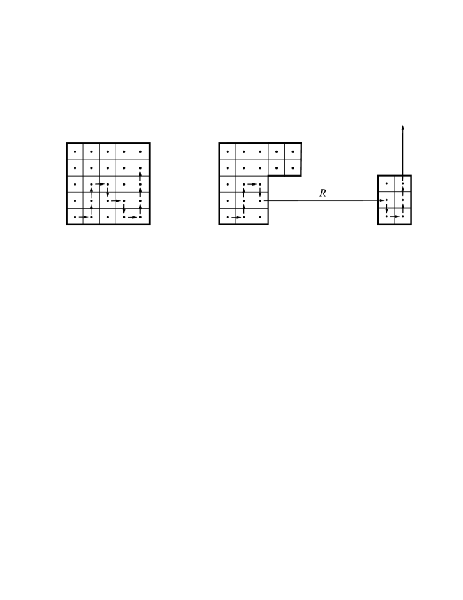
Figure 1: The coarse-grained trajectory in regular (left panel) and fractal (right panel) medium.

However, the strongly turbulent high magnetic field is not inherent in each cell. According to the current representation, which was formed five decades ago, most of the space between magnetic clouds is filled with lower quieter fields whose smooth field lines can hold individuality at a long distance. The charged particles of CRs move along these field lines in helical paths and from time to time enter trap clouds, where they can stay for a long time and “forget” their initial direction of motion. In this case, a jump from one trap to another is not instantaneous as in the above case: the particle rather intersects “almost empty” cells, covering large distances $R$. The distribution of $R$ in a fractal medium involves a long power-law tail. These transitions require the consideration of a finite velocity of the particle, more precisely, the leading center of the particle.

3 The bounded anomalous diffusion model

The most important consequence of the finiteness of the velocity of free particles is the finiteness of the spatial distribution: the probability density beyond a sphere with the radius $vt$ and the center at the instantaneous point source is zero in this case. Let us refer to this process as bounded anomalous diffusion in order to distinguish it from unbounded anomalous diffusion in which the motion of a particle is represented as a sequence of instantaneous jumps from one point of space to another: the particle arrives at the latter point at the same time at which it leaves the former point at any distance between these two points. The delay time (in a trap) is not related to this distance and to the motion as a whole. If the traps are removed from this model, it becomes senseless, because the particle instantaneously flies to infinity and leaves the system under consideration. The bounded anomalous diffusion model involves not only the time spent in the traps, but also the time taken for the motion of the particle and, for this reason, is meaningful even in the absence of traps. Finally, since the bounded anomalous diffusion propagator vanishes beyond the sphere with the radius $vt$, all of its moments are finite.

The effect of the finiteness of the velocity of free motion on the walk process described above, which was investigated in [Uchaikin (1998a), Uchaikin (1998b), Uchaikin (1998c), Uchaikin (1998d), Zolotorev et al. (1999), Uchaikin & Yarovikova(2003)], significantly changes the continuous time random walk model. In this case, the particle at the observation time can be in one of two states, rest and motion. The corresponding components of the probability density are denoted as $\psi_{0}(\mathbf{r},t)$ and $\psi_{1}(\mathbf{r},t)$ so that the total density is

$$\psi(\mathbf{r},t)=\psi_{0}(\mathbf{r},t)+\psi_{1}(\mathbf{r},t).$$

The rates of the $1\to 0$ and $0\to 1$ transitions per unit volume near the point $\mathbf{r}$ are denoted as $F_{1\to 0}(\mathbf{r},t)$ and $F_{0\to 1}(\mathbf{r},t)$, respectively. It is obvious that the particle passing to the state of rest at the point $\mathbf{r}$ at the time $t-t^{\prime}$ remains in this state at the observation time $\mathbf{t}$ with the probability $Q(t^{\prime})=\int_{t^{\prime}}^{\infty}q(t)dt$, and the particle leaving the trap at the point $\mathbf{r}\mathbf{r}^{\prime}$ intersects a unit area at the point $\mathbf{r}$ without an interaction with the probability $P(\mathbf{r}^{\prime})=\int_{0}^{\infty}p(\mathbf{r}^{\prime}+\xi\mathbf{\Omega})d\xi,\quad\mathbf{\Omega}=\mathbf{r}^{\prime}/r^{\prime}.$ Since this transition takes $r^{\prime}/v$ seconds,

$$\psi(\mathbf{r},t)=\int\limits_{0}^{\infty}dt^{\prime}Q(t^{\prime})F_{1\to 0}(\mathbf{r},t-t^{\prime})+v^{-1}\int d\mathbf{r}^{\prime}P(\mathbf{r}^{\prime})F_{0\to 1}(\mathbf{r}-\mathbf{r}^{\prime},t-r^{\prime}/v),$$

The factor $v^{-1}$ appears in front of the integral because the integral gives the flux of particles, whereas $\psi_{1}$ is the concentration of these particles. The transition rates (if the particle begins its evolution in a trap at the origin of the coordinates at the initial time) are related as

$$F_{1\to 0}(\mathbf{r},t)=\int d\mathbf{r}^{\prime}p(\mathbf{r}^{\prime})F_{0\to 1}(\mathbf{r}-\mathbf{r}^{\prime},t-r^{\prime}/v)+\delta(\mathbf{r})\delta(t),$$

$$F_{0\to 1}(\mathbf{r},t)=\int\limits_{0}^{\infty}d\tau q(\tau)F_{1\to 0}(\mathbf{r},t-\tau),$$

The Fourier Laplace transformation

$$\psi(\mathbf{r},t)\mapsto\psi(\mathbf{k},\lambda)=\int d\mathbf{r}\int\limits_{0}^{\infty}e^{i\mathbf{k}\mathbf{r}-\lambda t}\psi(\mathbf{r},t)dt$$

reduces the system of Eqs. (3)-(5) to the form

$$L_{v}(\lambda,\mathbf{k})\psi(\mathbf{k},\lambda)\equiv[1-p(\mathbf{k},\lambda/v)q(\lambda)]\psi(\mathbf{k},\lambda)=S_{v}(\lambda,\mathbf{k}),$$

where

$$S_{v}(\lambda,\mathbf{k})=Q(\lambda)+(1/v)P(\mathbf{k},\lambda/v)q(\lambda)$$

and

$$p(\mathbf{k},\lambda/v)=\int p(\mathbf{r})e^{-(\lambda/v)r}e^{i\mathbf{k}\mathbf{r}}d\mathbf{r}.$$

The quantity $P(\mathbf{k},\lambda/v)$ is determined similarly. If the tails of the distributions of $R$ and $T$ are of a power-law character with exponents $\alpha\in(0,2)$ and $\beta\in(0,1]$, respectively,

$$\textsf{P}(R>r)\sim\frac{A}{\Gamma(1-\alpha)}r^{-\alpha},\ r\to\infty,\qquad\textsf{P}(T>t)=Q(t)\sim\frac{B}{\Gamma(1-\beta)}t^{-\beta},\ t\to\infty.$$

Then, using Tauberian theorems, one can show that for $\mathbf{k}\to 0,\ \lambda\to 0$

$$L_{v}(\lambda,\mathbf{k})\sim B\lambda^{\beta}+\left\{\begin{array}[]{ll}\langle R\rangle\langle\lambda/v-i\mathbf{k}\mathbf{\Omega}\rangle+A\langle(\lambda/v-i\mathbf{k}\mathbf{\Omega})^{\alpha}\rangle,&\alpha>1,\\ A\langle(\lambda/v-i\mathbf{k}\mathbf{\Omega})^{\alpha}\rangle,&\alpha<1.\\ \end{array}\right.$$

where $\mathbf{\Omega}$ is a random direction of the motion, which is assumed to be isotropically distributed. The comparison of different terms at $\lambda\to 0$ provides the following conclusions.

The asymptotic expressions at $v=\infty$ for both cases have the same form

$$L_{v}(\lambda,\mathbf{k})\sim B[\lambda^{\beta}+C_{\infty}|\mathbf{k}|^{\alpha}],\qquad C_{\infty}=A|\cos(\alpha\pi/2)|/[(\alpha+1)B],$$

This expression provides fractional differential equation (1) of unbounded anomalous diffusion. At $v<\infty,\ \alpha=2,\ \beta=1$ (in view of the mentioned isotropy, $\langle\mathbf{\Omega}\rangle=0$), the transport operator has the form

$$L_{v}(\lambda,\mathbf{k})\sim B\lambda^{\beta}+\langle R\rangle\langle\lambda/v-i\mathbf{k}\mathbf{\Omega}\rangle+A\langle(\lambda/v-i\mathbf{k}\mathbf{\Omega})^{2}\rangle=(A/v^{2})\lambda^{2}+(B+\langle R\rangle/v)\lambda-(A/3)k^{2},$$

corresponding to the telegraph equation

$$\left[\frac{A}{v^{2}}\frac{\partial^{2}}{\partial t^{2}}+\left(B+\frac{\langle R\rangle}{v}\right)\frac{\partial}{\partial t}-\frac{A}{3}\triangle\right]\psi(\mathbf{r},t)=S_{v}(\mathbf{r},t),$$

which describes the bounded normal diffusion. Under the same conditions at $\beta<1$, the following fractional variant of the subdiffusion telegraph equation is obtained:

$$\left[\frac{A}{v^{2}}\frac{\partial^{2}}{\partial t^{2}}+\frac{\langle R\rangle}{v}\frac{\partial}{\partial t}+B\ _{0}\textsf{D}_{t}^{\beta}-\frac{A}{3}\triangle\right]\psi(\mathbf{r},t)=S_{v}(\mathbf{r},t).$$

In both bases, the form of the ”deep” time asymptotic expression for $\psi(\mathbf{r},t)$ is independent of the velocity and leads to the equations of bounded diffusion and subdiffusion, respectively. The same property is observed at $\alpha<1$ when $\beta<\alpha$. If $\alpha<\beta\leq 1$ (this relation between the parameters is used by Lagutin and Tyumentsev), the asymptotic equation for $\psi(\mathbf{r},t)$ has the form unusual for a diffusion process with a pseudodifferential operator $(\textsf{D}_{t}+v\mathbf{\Omega}\nabla)^{\alpha}$ averaged over the directions

$$(A/v^{\alpha})\langle(\textsf{D}_{t}+v\mathbf{\Omega}\nabla)^{\alpha}\rangle\psi(\mathbf{r},t)=S_{v}(\mathbf{r},t).$$

Here, the operator

$$\left(\textsf{D}_{t}+v\mathbf{\Omega}\nabla\right)^{\nu}\psi(\mathbf{r},t)=\frac{1}{\Gamma(1-\nu)}\left(\textsf{D}_{t}+v\mathbf{\Omega}\nabla\right)\int\limits_{0}^{t}\frac{\psi(\mathbf{r}-v\mathbf{\Omega}(t-\tau),\tau)}{(t-\tau)^{\nu}}d\tau$$

is the fractional generalization of the material derivative that is agree with results obtained by [Sokolov & Metzler(2003)] for one-dimensional Lévy walks.

If we consider the case of homogeneous distribution of particles $\psi(\mathbf{r},t)\equiv\psi(\mathbf{t})$ this operator becomes the fractional Rieman-Liouville derivative with respect to time:

$$\left(\textsf{D}_{t}+v\mathbf{\Omega}\nabla\right)^{\nu}\psi(\mathbf{r},t)\mapsto\ _{0}\textsf{D}^{\nu}_{t}\psi(\mathbf{t})$$

In the stationary problem, when the function $\psi(\mathbf{r},t)=\psi(\mathbf{r})$ does not depend on time,

$$\left(\textsf{D}_{t}+v\mathbf{\Omega}\nabla\right)^{\nu}\psi(\mathbf{r})\mapsto\ \left(v\mathbf{\Omega}\nabla\right)^{\nu}\psi(\mathbf{r}),$$

this operator represents fractional generalization of directional derivative.

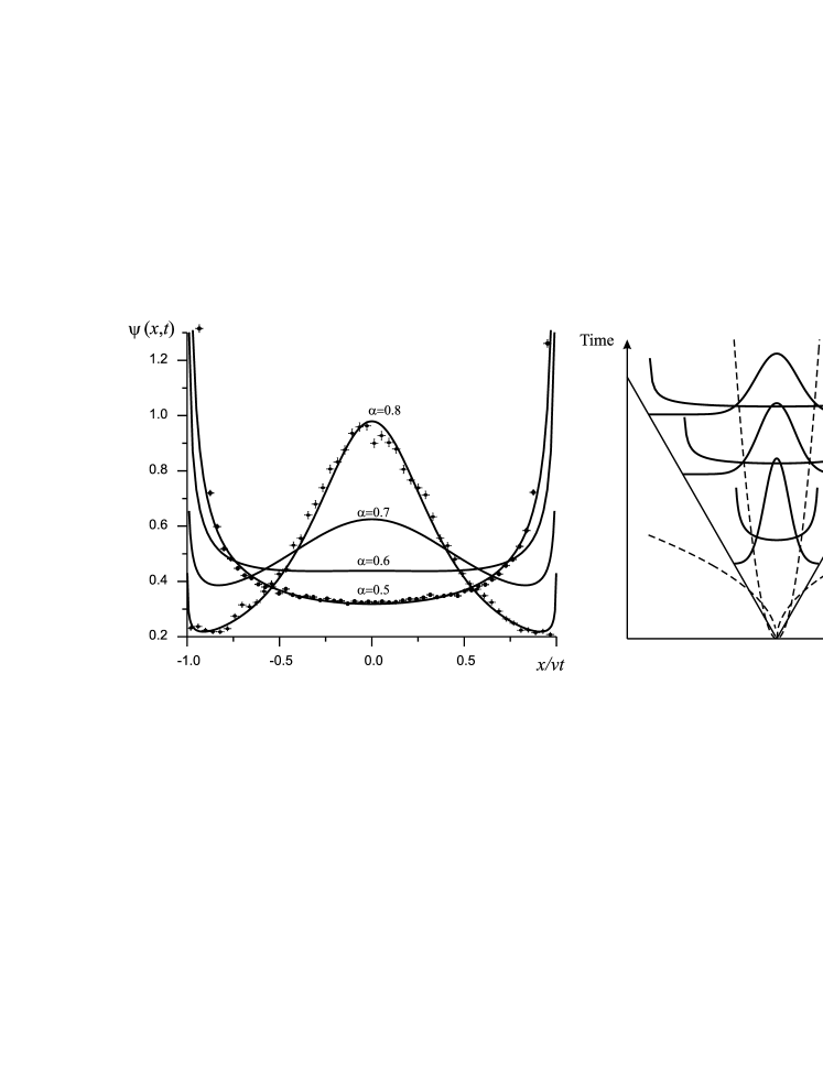
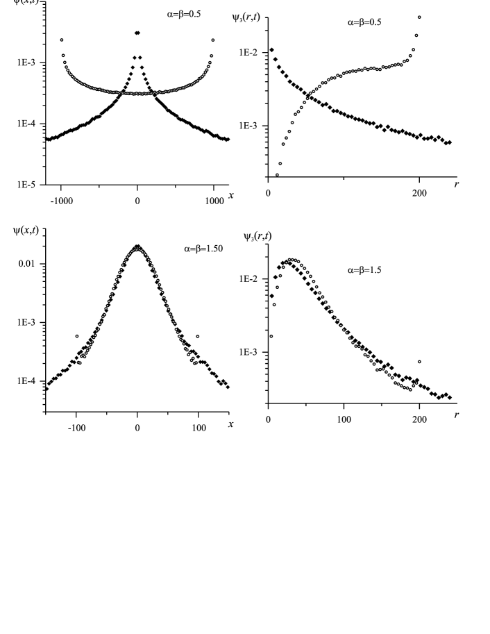
Figure 2: Comparison of analytical solutions (lines) with results of numerical Monte Carlo simulation (points) in one-dimensional case (left panel). Evolution of the Gaussian diffusion packet and the propagator of the bounded anomalous diffusion model, $\alpha=0.5$ (right panel). Dashed lines represent the time dependencies of the diffusion packet width in both cases.

Figure 3: Comparison of propagators of the bounded anomalous diffusion (circles) and unbounded diffusion (rhombs) for $\alpha=0.5$ and 1.5 in the 1D case (left panel) and 3D case (right panel).

The dependence on the velocity remains at any time, but the dependence on disappears. The distribution $\psi(\mathbf{r},t)$ corresponding to this case has a specific $U$ shape in the region bounded by the radius $vt$ beyond which it vanishes (see [Zolotorev et al. (1999), Uchaikin & Yarovikova(2003)]).

4 The bounded anomalous diffusion propagator

In one-dimensional case, for $\alpha<1$, the equation of bounded anomalous diffusion without traps takes the form:

$$\left[\left(\frac{\partial}{\partial t}-v\frac{\partial}{\partial x}\right)^{\nu}+\left(\frac{\partial}{\partial t}+v\frac{\partial}{\partial x}\right)^{\nu}\right]\Phi(x,t)=\frac{t^{-\nu}}{2\Gamma(1-\nu)}\ [\delta(x-vt)+\delta(x+vt)],$$

Solutions of this equation can be expressed through elementary functions (see [Uchaikin & Sibatov(2009)])

$$\Phi(x,t)=\frac{2\sin\pi\nu}{\pi}\frac{\left(1-x^{2}/v^{2}t^{2}\right)^{\nu-1}}{(1-x/vt)^{2\nu}+(1+x/vt)^{2\nu}+2\left(1-x^{2}/v^{2}t^{2}\right)^{\nu}\cos\pi\nu}.$$

Solutions can also be written in terms of fractional stable densities (see [Uchaikin & Sibatov(2009)]), that are useful for probabilistic interpretation of these distributions.

In Fig. 2 (left panel), the analytical solutions (lines) are compared with the results of Monte Carlo simulated random walks with finite velocity of motion (points). In Fig. 2 (right panel), the influence of ballistic restriction on the dynamics of diffusion packet spreading is demonstrated schematically.

To make clear the role of correlations between path lengths and waiting times in the model under consideration, we compare propagators of bounded and unbounded anomalous diffusion. In the latter model we take identical distributions for waiting times and path lengths ($\alpha=\beta$). In the model of unbounded anomalous diffusion path lengths and waiting times in traps are independent. We take the model of bounded anomalous diffusion without traps, time delay is provided by finiteness of rays propagation velocity ($v=1$). The results for the one-dimensional case are presented in Fig. 3 (left panel), and for the 3D-model in the right panel. From the graphs, we can see that distinction in kind between propagators disappears only when $\alpha=\beta>2$. For values $\alpha=\beta\leq 1$, distinctions are very strong, shapes of packets, spreading laws, behaviors near the ballistic boundaries and near the source are essentially different. When $1<\alpha=\beta<2$, distinctions are also sufficient despite the fact that mean path length is finite. In one case distributions are bounded, in another case they are unbounded. In the model of bounded anomalous diffusion, the front near $|\mathbf{r}|=vt$ appears. The densities differ quantitatively near the source as well. All these facts say that the results obtained on the base of unbounded anomalous diffusion and presented in the works [Lagutin et al. (2001), Lagutin & Uchaikin (2001), Lagutin & Uchaikin (2003), Lagutin & Tyumentsev (2004), Lagutin et al. (2009)] need to be re-examined.

5 Concluding remarks

The work ([Zolotorev et al. (1999)], p. 1424) on anomalous diffusion ended with the phrase: ”The last property can be a reason for the conclusion that the superdiffusion equation is inapplicable to the description of real physical processes with the characteristic exponents $\alpha<1$” . The cautious word “can” is not accidental here: if the walk of the particle is considered in the space of, e.g., velocities or momenta, an instantaneous jump of the particle at large “distance” is allowable and even justified in the framework of the commonly accepted model of instantaneous collisions. The use of the model with an infinite velocity of particles without any boundary conditions to describe the walk of the particles in the coordinate space at $\alpha\leq\beta$ makes both the results and conclusions doubtful (in particular, the conclusion that “the self-consistent description of the experimental data on the spectra of individual groups of nuclei and the spectrum of all of the particles is not achieve” [Lagutin et al. (2009)] p. 601). We hope that taking into account the finiteness of the propagation velocity of CRs in the framework of the bounded anomalous diffusion proposed in this work will be more fruitful.

References

- [Balescu (1995)] R. Balescu. Anomalous transport in turbulent plasmas and continuous time random walks. Phys. Rev. E, 51:4807–4822, 1995.
- [Berezinskij(1990)] V. S. Berezinskij, S. V. Bulanov, V. L. Ginzburg, V. A. Dogiel, V. S. Ptuskin. Astrophysics of Cosmic Rays. Nauka, Moscow, 1990.
- [Chukbar & Zaburdaev(2003)] K. V. Chukbar, V. Yu. Zaburdaev. Comment on ”Towards deterministic equations for Lévy walks: The fractional material derivative”. Phys. Rev. E, 68:033101, 2003.
- [Chuvilgin & Ptuskin (1993)] L. G. Chuvilgin, V. S. Ptuskin. Anomalous diffusion of cosmic rays across the magnetic field. Astron. Astrophys., 279:278–297, 1993.
- [Dorman (1975)] L. I. Dorman. Experimental and Theoretical Basement of Cosmic Rays Astrophysics. Nauka, Moscow, 1975.
- [Erlykin & Wolfendale (1997)] A. D. Erlykin, A. W. Wolfendale. A single source of cosmic rays in the range-ev. J. Phys. G: Nucl. Par. Phys., 23:979–989, 1997.
- [Ketabi(2009)] N. Ketabi, J. Fatemi. A simulation on the propagation of supernova cosmic particles in a fractal medium. Transaction B: Mechanical Engineering, Sharif University of Technology, 16(3):269–272, 2009.
- [Kolokoltsov et al. (2000)] V. Kolokoltsov, V. Korolev, V. Uchaikin. Fractional stable distributions. Res. Report No 23/00, The Nottingham Trent University, UK, 2000.
- [Kulakov & Rumjantsev (1994)] A. V. Kulakov, A. A. Rumjantsev. Fractals and energy spectrum of fast particles. Reports of the Russian Academy of Sciences, 336:183–185, 1994.
- [Lagutin et al. (2001)] A. A. Lagutin, Yu. A. Nikulin, V. V. Uchaikin. The ”knee” in the primary cosmic ray spectrum as consequence of the anomalous diffusion of the particles in the fractal interstellar medium. Nuclear Physics B (Proc. Suppl.), 97:267–270, 2001.
- [Lagutin & Uchaikin (2001)] A. A Lagutin, V. V. Uchaikin. Fractional diffusion of cosmic rays. Proc. of 27th ICRC (Hamburg), 5:1896–1899, 2001.
- [Lagutin & Uchaikin (2003)] A. A. Lagutin, V. V. Uchaikin. Anomalous diffusion equation: Application to cosmic ray transport. Nuclear Instr. and Meth. in Physics Research, B201:212–216, 2003.
- [Lagutin & Tyumentsev (2004)] A. A. Lagutin, A. G. Tyumentsev. Spectr, mass-composition and anisotropy of cosmic rays in a fractal galaxy. Bulletin of Altai State University, 5:4–21, 2004.
- [Lagutin et al. (2009)] A. A. Lagutin, A. G. Tyumentsev, N. V. Volkov. Cosmic ray spectrum in a fractal-like galactic medium for different particle acceleration mechanisms in a source. Bulletin of the Russian Academy of Sciences: Physics, 73(5):599–601, 2009.
- [Monin (1955)] A. S. Monin. The turbulent diffusion equations, reports of the ussr academy of sciences. Reports of the USSR Academy of Sciences, 105:256–259, 1955.
- [Montroll & Weiss (1965)] E. W. Montroll, G. H. Weiss. Random walk on lattices II. J. Math. Phys., 6:167–182, 1965.
- [Ragot & Kirk (1997)] B. R. Ragot, J. G. Kirk. Anomalous transport of cosmic ray electrons. Astron. Astrophys., 327:432–440, 1997.
- [Ruzmaikin et al. (1988)] A. A. Ruzmaikin, A. M. Shukurov, D. D. Sokolov. Magnetic Fields of Galaxies. Kluwer, Dordrecht, 1988.
- [Saichev & Zaslavsky (1997)] A. I. Saichev, G. M. Zaslavsky. Fractional kinetic equations: solutions and applications. Chaos, 7(4):753–764, 1997.
- [Sokolov & Metzler(2003)] I. M. Sokolov, R. Metzler. Towards deterministic equations for Lévy walks: The fractional material derivative. Phys. Rev. E, 67:010101 (R), 2003.
- [Uchaikin (1998a)] V. V. Uchaikin. Renewal theory for anomalous transport processes. J. Math. Phys., 92(4):4085–4096, 1998.
- [Uchaikin (1998b)] V. V. Uchaikin. Anomalous transport equations and their application to fractal walking. Physica A, 255/1-2:65–92, 1998.
- [Uchaikin (1998c)] V. V. Uchaikin. Anomalous diffusion of particles with a finite free-motion velocity. Physica A, 115(1):496–501, 1998.
- [Uchaikin (1998d)] V. V. Uchaikin. Anomalous transport of particles with finite speed and asymptotical fractality. Journ.Techn.Phys., 68(1):138–139, 1998.
- [Uchaikin & Zolotarev (1999)] V. V. Uchaikin, V. M. Zolotarev. Chance and Stability. Stable Distributions and their Applications. VSP, Utrecht, the Netherlands, 1999.
- [Uchaikin & Yarovikova(2003)] V. V. Uchaikin, I. V. Yarovikova. Numerical solution of the time-dependent problem of anomalous finite-velocity diffusion by the moment method. Computational Mathematics and Mathematical Physics, 43(10):1478–1490, 2003.
- [Uchaikin & Sibatov(2004)] V. V. Uchaikin, R. T. Sibatov. One-dimensional fractal walk at a finite free motion velocity. Techn. Phys. Lett., 30:316- 318, 2004.
- [Uchaikin(2008)] V. V. Uchaikin. The Method of the Fractional Derivatives. Artishok, Ulyanovsk, 2008.
- [Uchaikin & Sibatov(2009)] V. V. Uchaikin, R. T. Sibatov. Statistical model of fluorescence blinking. Journal of Exper. and Theor. Physics, 109:537- 546, 2009.
- [Webb et al. (2006)] G. M. Webb, G. P. Zank, E. Kh. Kaghashvili. Compound and perpendicular diffusion of cosmic rays and random walk of the field lines. I. Astrophys. Journal, 651:211–236, 2006.
- [Zolotorev et al. (1999)] V. M. Zolotorev, V. V. Uchaikin, V. V. Saenko. Superdiffusion and stable laws. Journal of Exper. and Theor. Physics, 88(4):780–783, 1999.
- [Zaburdaev & Chukbar(2002)] V. Yu. Zaburdaev, K. V. Chukbar. Accelerated superdiffusion and finite velocity of Lévy walks. Journal of Exper. and Theor. Physics, 121:299–307, 2002.