Statistical Complexity of
Sampled Chaotic Attractors

Abstract

We analyze the statistical complexity vs. entropy plane-representation of sampled chaotic attractors as a function of the sampling period $\tau$. It is shown that if the Bandt and Pompe procedure is used to assign a probability distribution function (PDF) to the pertinent time series, the statistical complexity measure (SCM) attains a definite maximum for a specific sampling period $t_{M}$. If the usual histogram approach is used instead in order to assign the PDF to the time series, the SCM remains almost constant at any sampling period $\tau$. The significance of $t_{M}$ is further investigated by comparing it with typical times given in the literature for the two main reconstruction processes: the Takens’ one in a delay-time embedding, and the exact Nyquist-Shannon reconstruction. It is shown that $t_{M}$ is compatible with those times recommended as adequate delay ones in Takens’ reconstruction. The reported results correspond to three representative chaotic systems having correlation dimension $2<D_{2}<3$. One recent experiment confirm the analysis presented here.

PACS: 05.45.-a 02.70.Rr 05.40.-a 07.05.-t;

Version: V2-15

1 Introduction

The study of randomness started with Poincaré, but it took almost $80$ years for digital electronics to make enough computational resources available so that the investigation on the transition from order to randomness could lead to the fascinating issue of deterministic chaos. One hallmark of chaotic systems is the presence of recognizable patterns in their state space. Pattern-formation plays a fundamental role in the definition of i) structural complexity by Crutchfield [1] and ii) a number of other complexity measures, such as the so-called statistical complexity (SCM), relevant for this paper. For an excellent review on complexity measures see [2]. The SCM, based on the notion of disequilibrium in Statistical Space, was proposed by López Ruiz, Mancini and Calbet [3] and improved upon later in several papers [4, 5, 6]. The SCM version employed here was advanced in [5]. In a related vein, the importance of using a “causal” Probability Distribution Function (PDF) to analyze the stochasticity-degree of chaotic and pseudo stochastic systems was emphasized in [6] and [7, 8, 9].

In this field of endeavor it is of importance to study just how the sampling period $\tau$-influences the final results given that digital instrumentation is widely used in concomitant experiments. The most common sampling criterion is given by the sampling theorem by Nyquist and Shannon [10, 11]. It stipulates that the exact reconstruction of a continuous signal is possible whenever its Fourier spectrum vanishes for frequencies above a certain $B=f_{max}$ (the bandwidth). An infinite number of regularly sampled values is required and $\tau$ must satisfy the inequality $\tau<t_{NS}=1/(2B)$ where $t_{NS}$ is the Nyquist-Shannon minimum sampling interval. The exact original continuous signal is recovered from the time series by using an ideal low pass filter. Note that in actual scenarios the number $N$ of samples is always finite and an exact reconstruction is not possible.

In a different vein, Takens [12] demonstrated that chaotic attractors generated by dynamical systems may be reconstructed if one has access to the infinite time series of regularly sampled values for just one state variable. Takens’ procedure allows one to obtain the main parameters characterizing the chaotic system, like Lyapunov exponents, dimensions, etc. For an impressive web-site containing very useful routines for nonlinear time series analysis see [13]. The ensuing reconstruction procedure uses “delayed-samples” with $t_{T}$ as the delay time, to generate a $d$-dimensional vector (in a $d$-dimensional embedding space). Note that the time delay $t_{T}$ must be a multiple of the sampling period $\tau$, since we only possess data gathered at those times. Let us remark that in the context of Takens’ theorem the vocable reconstruction adopts a different meaning than that assigned by the Nyquist-Shannon theorem. In this paper we differentiate between a Takens reconstruction and a Nyquist reconstruction. We will carefully look at just how the representative point of a chaotic attractor in an entropy-complexity plane ($H\times C$) changes with the sampling period. It will be shown that when the causal PDF prescribed by the Bandt and Pompe procedure [14] is used, the ensuing complexity $C=C^{(BP)}$ exhibits a maximum for a given sampling period $\tau=t_{M}$. However, such maximum does not appear if the conventional histogram-approach is used instead in assigning a PDF to the time series and thus a $C=C^{(hist)}$ is used. We call the later histogram-distribution a non-causal PDF. In point of fact, that of causality constitutes a difficult topic (see for instance [15]). In this paper a causal PDF is one that takes into account the temporal correlation between successive samples, which entails using a PDF with a symbol assigned to each trajectory’s piece of length $L=d\cdot\tau$.

It is of interest, for both the Takens and the Nyquist-Shannon reconstruction processes, to analyze the relation between i) $t_{M}$ and ii) other related temporal quantities proposed in the literature such as $t_{T}$ or $t_{NS}$. This is one of the topics to be here investigated. In the case of Takens’ reconstruction it is well known that for a finite number of samples $N$ the quality of the reconstruction requires the selection of an adequate value for $t_{T}$. There exist in the literature several different recommendations for a “good” $t_{T}$, like the first zero of the autocorrelation function, the first minimum of the mutual information function, etc. [16]. For an interesting discussion see [17, 18]. In the case of Nyquist’s reconstruction, a bandwidth criterium must be chosen in order to evaluate the Nyquist-Shannon time $\tau=t_{NS}$ (because the spectrum of chaotic systems is not band-limited).

In Section 2 we review the Takens embedding theorem and the delay embedding reconstruction process. Section 3 deals with the Nyquist-Shannon reconstruction process. In Section 4 the specific SCM used in the paper is reviewed. Results for three paradigmatic examples: (a) the Lorenz Chaotic Attractor; (b) the Rössler Chaotic Attractor and (c) the chaotic attractor named ${\mathbf{B}}_{7}$ by Chlouverakis and Sprott [19] are reported in Section 5. The first two attractors have been extensively studied in the literature but they both have a correlation dimension $D_{2}\approx 2$ while the attractor ${\mathbf{B}}_{7}$ has $D_{2}\approx 2.719$, covering almost all the $3D$ state-space. Conclusions and remarks are included in Section 6. It is interesting to remark that the analysis performed here has been experimentally verified [20].

2 Takens’ embedding theorem

Let $d\mathbf{x}/dt=\mathbf{f}(\mathbf{x})$ be an $m$-dimensional continuous dynamical system. A scalar measurement $s(t)\equiv s(\mathbf{x}(t))$ is a projection of the state $\mathbf{x}$ onto an interval $I\in\mathbb{R}$. The goal of all the embedding theorems proposed in the literature is to obtain a $d$-dimensional embedding space $\mathfrak{A}$ in which $\mathbf{x}(t)$ can be reconstructed by using only $s(t)$. This reconstruction does not need to be exact, especially in the case of chaotic dissipative systems that usually have attractors with box counting dimension $D_{BC}$ smaller than $m$, the dimension of the state space. In this context, reconstruction merely indicates that $\mathbf{\widetilde{x}}(t)\in\mathfrak{A}$ shares with $\mathbf{x}(t)$ some characteristics. The main requirements a reconstructed space must fulfill are:

1. Uniqueness of the dynamics in the reconstructed space.

2. The reconstructed attractor must have dimensions, Lyapunov exponents and entropies identical to those of the original attractor.

Consequently, the embedding of a compact smooth manifold $A$ into $\mathbb{R}^{d}$ is defined to be a one-to-one $\mathfrak{C}^{1}$ map $\mathcal{F}$, with a Jacobian $DF(\mathbf{x})$ which has full rank everywhere. Let us assume that an infinite length-time scalar series $\{s_{n};n=1,2,\cdots,\infty\}$ is obtained by measuring one component of the $m$-dimensional vector field at evenly spaced times $t_{n}=n\cdot\tau$, with $\tau$ the sampling period. A time-delayed vector field is constructed as follows:

$${\widetilde{x}}^{(1)}_{n}=s_{n}~{};\;{\widetilde{x}}^{(2)}_{n}=s_{n+1}~{};\;\cdots~{};\;{\widetilde{x}}^{(d)}_{n}=s_{n+d-1}\ .$$ (1)

Takens proved [12] that time-delay maps of dimension $2d+1$ have the generic property of being the embedding of a compact manifold with dimension $d$, if: (1) the measurement function $s:A\rightarrow\mathbb{R}$ is $\mathfrak{C}^{2}$ and (2) either the dynamics or the measurement couples all degrees of freedom. In the original version by Takens, $d$ is the integer dimension of a smooth manifold, the phase space containing the attractor. Thus $d$ can be much larger than the attractor dimension. Sauer et al. [21] were able to generalize the theorem into what they call the Fractal Delay Embedding Prevalence Theorem. Let $D_{BC}$ be now the box counting dimension of the (fractal) attractor. Then, for almost every smooth measurement function $s$ and any sampling time $\tau>0$, the delay map into $\mathbb{R}^{d}$ with $d>2D_{BC}$ is an embedding if: (1) there are no periodic orbits of the system with period $\tau$ or $2\tau$ and (2) there only exists a finite number of periodic orbits with period $p\tau$, with $p>2$. Thus the main result of the embedding theorems is that it is not the dimension $m$ of the underlying state space what is important for ascertaining the minimal dimension of the embedding space, but only the fractal dimension $D_{BC}$ of the support of the invariant measure generated by the dynamics in the state space. In dissipative systems $D_{BC}$ can be much smaller than $m$. Let us further remark that in favorable cases an attractor might be reconstructed in spaces of dimension $d$ such that $D_{BC}\leq d\leq 2D_{BC}$. For example, for the determination of the correlation dimension, events of measure zero can be neglected; thus any embedding with a dimension larger that $D_{BC}$ is sufficient.

From a mathematical point of view, and for an infinite number of data items (known with infinite precision as assumed in embedding theorems), the time-delay $t_{T}$ is an arbitrary multiple of $\tau$. Thus, there exists no rigorous way of determining $t_{T}$’s optimal value. But in a real scenario with a finite number $M$ of data items, the specific value adopted by the time delay is quite important. Moreover, it is even unclear what properties the optimal value should have for best estimating a continuous system’s specific property. Many different methods have been suggested to estimate the time-delay [13, 18, 22, 23]. In the case of Takens’ reconstruction procedure it is possible to use a time delay $t_{T}>\tau$ as pointed out above. Since in this paper the sample period $\tau$ will be movable we will consider that both times are equal ($t_{T}=\tau$).

The analysis of (i) linear autocorrelations and (ii) average mutual information for a time series are two of the criteria often used in the literature to determine the best $t_{T}$-region. Several characteristic times have been recommended using these two types of analysis. Let us recapitulate.

1. Time-delays induced by the discrete linear autocorrelation function. Let ${\mathcal{S}}\equiv\{s(n);n=1,\cdots,M\}$ be the measured component of the vector field (the time series). The discrete linear autocorrelation function is a vector $R_{i}$ defined as:

   $$R_{i}~{}=~{}\frac{1}{M}~{}\sum_{n=0}^{M-i-1}[s({n+i})-<s>]\cdot[s(n)-<s>]\ ,$$ (2)

   with $<s>=\sum_{i=1}^{M}s_{i}$ the mean value for the time series.
   

   Four characteristic time delays are considered here:

   1. The first zero crossing of $R_{i}$ (if it exists). Let $\tau$ and $i_{0}$ be, respectively, the sampling period and the first zero crossing of $R_{i}$. The characteristic time is $t_{0}~{}=~{}i_{0}~{}\tau$.

   2. The first zero crossing of $R^{\prime}_{i}~{}=~{}R_{i+1}-R{{}_{i}}$ gives the first minimum of $R$. We call this characteristic time $t_{1}=i_{1}~{}\tau$.

   3. The first zero crossing of $R^{\prime\prime}_{i}~{}=~{}R^{\prime}_{i+1}-R^{\prime}_{i}$ yields the first curvature-change of $R$. We call this characteristic time $t_{2}=i_{2}~{}\tau$.

   4. Let $i=i_{1/e}$ be the smallest $i$ making $R_{i}$ to decay to less than $R_{0}/e$. The corresponding characteristic time is $t_{1/e}=i_{1/e}~{}\tau$.
      

2. Delay-time induced by the discrete Mutual Information function. Let ${\mathcal{S}}\equiv\{s(n);n=1,\cdots,M\}$ be the measured component of the vector field (the time series). The discrete Mutual Information function is a vector $I_{i}$, defined as:

   $$I_{i}=~{}-\sum_{k,l}p_{kl}(s(n),s(n+i))\ln\left[\frac{p_{k,l}(s(n),s(n+i))}{p_{k}(s(n))\cdot p_{l}(s(n+i))}\right]\ .$$ (3)

Equation (3) is determined as follows: (a) the real interval $[a,b]$ covered by the time series is partitioned into $N_{box}$ subintervals, equal sized consecutive non overlapping subintervals; (b) $p_{k}$ is the probability to find a time series’ value, $s(n)$, in the $k$-th interval, and $p_{k,l}$ is the joint probability for simultaneously encountering a time series’ value, $s(n)$, in the $k$-th interval while the time series’ value found at the $i$-th posterior positions, $s(n+i)$, falls into the the $l$-th interval. This quantity can be quite easily computed, for sufficiently small sizes of the partition elements (sufficiently high values of $N_{box}$), and, provided the attractor dimension is $\leq 2$, this expression has no systematic dependence on $N_{box}$ [18, 24].

There exist good arguments for asserting that, if the time-delayed mutual information exhibits a marked minimum for a certain value of the delay $i_{I}$, then this is a good candidate for a “reasonable” time delay. The corresponding characteristic time is given by $t_{I}~{}=~{}i_{I}~{}\tau$. Nevertheless when one finds that the minimum of the mutual information $t_{I}$ lies at considerably larger times than $t_{1/e}$ (the decay of autocorrelation function), it is worth optimizing the time-lag inside this range [18].

3 Nyquist-Shannon theorem and the minimum sampling time

The well known Nyquist-Shannon sampling theorem [10, 11] is based on the Fourier Transform (FT). It states that a function $s(t)$, $t\in[-\infty,\infty]$, containing no frequencies higher than $B$ in its FT, is completely determined by giving its coordinates at an infinite series of points (samples) spaced $\tau~{}<~{}t_{NS}=1/(2B)$ apart.

Consider the case of chaotic signals that are not band-limited. A value of $B$ may be defined from the Discrete FT as follows. Let $\{S\}$, be the Discrete FT (DFT) of $\{s\}$ defined by

$$S_{k}~{}=~{}\sum_{j=1}^{M}s_{j}~{}e^{-i\;2\pi(j-1)(k-1)/M}\ .$$ (4)

The power contained in the first $i$ frequency components of the DFT’s is given by

$$PW_{i}=\sum_{k=1}^{i}S_{k}~{}S^{*}_{k},$$ (5)

where ^∗ refers to complex conjugation while the index $i\leq M$. The full power $PW$ is given by Eq. (5) with $i=M$. To define $B$ we choose the value $i=i_{\alpha}$ in such a way as to make $PW_{i_{\alpha}}=\alpha PW$. The maximum frequency $B$ for such $\alpha-$value is then defined as $B=i_{\alpha}/\tau$. Once this maximum frequency is obtained, the Nyquist-Shannon criterion prescribes that $t_{NS}^{(\alpha)}=1/(2B)$. Our present calculations were made with $0.80\leq\alpha\leq 0.99$.

4 The Statistical Complexity Measure $C$ using Bandt and Pompe’s prescription

The SCM $C$ is an informational quantifier. As such, it is a functional of a probability distribution function (PDF). In this case we refer to an appropriate PDF associated with a time series. Given the PDF, $P\equiv\{p_{i};i=1,\cdots,N\}$, there are several manners to obtain the functional and a full discussion of the subject would exceed the scope of this presentation (for a comparison amongst different complexity measures see the excellent paper by Wackerbauer et al. [2]).

In the present work we adopt for the SCM the functional form introduced in López Ruiz-Mancini-Calbet seminal paper [3] with the modifications advanced by Lamberti et al. [5]. This functional form is an intensive (in a thermodynamics sense) statistical complexity $C[P]$ given by

$$C[{P}]=Q_{J}[{P,P_{e}}]\cdot H[{P}]\ ,$$ (6)

where $H$ denotes the amount of “disorder” given by the normalized Shannon entropy

$$H[P]=S[P]/S_{max},$$ (7)

and $Q_{J}$ is the so-called “disequilibrium”, defined in terms of the extensive Jensen-Shannon divergence (which induces a squared metric) [5]:

$$Q_{J}[{P,P_{e}}]=Q_{0}\cdot J[P,P_{e}]=Q_{0}\cdot\{S[(P+P_{e})/2]-S[P]/2-S[P_{e}]/2\}\ .$$ (8)

In these equations $P_{e}=\{1/N,\cdots,1/N\}$ stands for the uniform distribution, while $S[P]=-\sum_{j=1}^{N}~{}p_{j}~{}\ln(p_{j})$ is the Shannon entropy corresponding to the PDF $P$. We use two normalization constants, namely,

$$S_{max}=S[P_{e}]=\ln N\ ,$$ (9)

and

$$Q_{0}=-2\left\{\left(\frac{N+1}{N}\right)\ln(N+1)-\ln(2N)+\ln N\right\}^{-1}\ .$$ (10)

The normalization constant $Q_{0}$ is equal to the inverse of the maximum possible value of $J[P,P_{e}]$. This value is obtained when one component of $P$, say $p_{m}$, is equal to one and all the remaining $p_{i}$’s are equal to zero. We have then $0\leq H\leq 1$ and $0\leq Q_{J}\leq 1$.

The disequilibrium $Q_{J}$ is an intensive thermodynamical quantity that reflects on the systems’ architecture, being different from zero only if there exist privileged, or more likely states among the accessible ones. $C[P]$ quantifies the presence of correlational structures as well [4, 5]. The opposite extremes of perfect order and maximal randomness possess no structure to speak of and, as a consequence, their $C[P]=0$. In between these two special instances a wide range of possible degrees of physical structure exist, degrees that should be reflected in the features of the underlying probability distribution.

The complexity measure constructed in this way is intensive, as many thermodynamic quantities [5]. We stress the fact that the above SCM is not a trivial function of the entropy because it depends on two different probabilities distributions, the one associated to the system under analysis, $P$, and the uniform distribution, $P_{e}$. Furthermore, it was shown that for a given $H$ value, there exists a range of possible SCM values [25]. Thus, it is clear that $C$ carries important additional information (related to the correlational structure between the components of the physical system) that is not contained in the entropic functional.

A detailed analysis of the $C$-behavior demonstrates the existence of bounds to $C$ that we called $C_{max}$ and $C_{min}$. These bounds can be systematically evaluated by recourse to a careful geometric analysis performed in the space of probabilities $\Omega$ [25]. The corresponding values of $C_{max}$ and $C_{min}$ depend only on the probability space’s dimension and, of course, on the functional form adopted by the amount of disorder $H$ and the disequilibrium $Q$. $H\times C$ diagrams are important and yield system’s information independently of the values that the different control parameters may adopt. The bounds also provide us with relevant information that depends on the system’s particular characteristics, as for instance, the existence of global extrema, or the peculiarities of the system’s configuration

As pointed out above, the PDF $P$ itself is not a uniquely defined object and several approaches have been employed in the literature to “associate” $P$ to a given time series. Just to mention some frequently used $P-$extraction (from the time series) procedures, one has: a) frequency counting [26], b) time series histograms [8], c) binary symbolic-dynamics [27], d) Fourier analysis [28], e) wavelet transforms [29, 30], f) partition entropies [31], g) discrete entropies [32], h) permutation (Bandt-Pompe) entropies [14, 33], among others. There is ample liberty to choose among them and the specific application must be carefully analyzed so as to make a good choice. Rosso et al. [6] showed that the last mentioned methodology may be profitably used in the plane $H\times C$ so as to separate and differentiate amongst stochastic, chaotic, and deterministic systems. It was shown in [34, 35] that temporal correlations are nicely displayed by the Bandt and Pompe PDF.

Summing up, different symbolic sequences may be assigned to a given time series. If one symbol $a$ of the finite alphabet $\mathfrak{A}$ is assigned to each $x_{t}$ of the time series, the symbolic sequence can be regarded as a non causal coarse grained description of the time series because the resulting PDF will not have any causal information. The usual histogram-technique corresponds to this kind of assignment. For extracting $P$ via an histogram one divides the interval $[a,b]$ (with $a$ and $b$ the minimum and maximum values in the time series) into a finite number $N_{bin}$ of non overlapping equal sized consecutive subintervals $A_{i}:[a,b]=\bigcup_{i=1}^{N_{bin}}A_{i}$ and $A_{i}\bigcap A_{j}=\emptyset~{}\forall i\neq j$.

Note that $N$ in equations (9) and (10) is equal to $N_{bin}$. Of course, in this approach the temporal order of the time-series plays no role at all. The quantifiers obtained via the ensuing PDF-histogram are called in this paper, respectively, $H^{(hist)}$ and $C^{(hist)}$. Let us also point out that for time series with a finite alphabet it is relevant to consider a judiciously chosen optimal value for $N_{bin}$ (see e.g. De Micco et al. [8]).

Causal information may be duly incorporated into the construction-process that yields $P$ if one symbol of a finite alphabet $\mathfrak{A}$ is assigned to a trajectory’s portion, i.e., we assign “words” to each trajectory-portion. The Bandt and Pompe methodology for extraction of the PDF corresponds to this type of assignment and the resulting probability distribution $P$ is thus a causal coarse grained description of the system. Note that, in the Bandt and Pompe approach a sort of coarse graining and word construction is effected (for methodological detail see below). Note that there are other ways to get a causal PDF. The advantage of the Bandt and Pompe approach lies in the fact that it solves the problem of finding generation partitions.

Thus one expect that for increasing patterns’ length (embedding dimension) the Bandt and Pompe approach retains all relevant essentials of the original continuous (in space) dynamics. The quantifiers obtained by appeal to this PDF are denoted in this paper as $H^{(BP)}$ and $C^{(BP)}$, respectively. A notable Bandt and Pompe result consists in yielding a clear improvement on the quality of Information Theory-based quantifiers [6, 7, 8, 9, 34, 35, 36, 37, 38, 39, 40, 41, 42, 43, 54, 44, 45, 46, 47].

In summarizing now the approach, note that Bandt and Pompe [14] introduced a simple and robust method to evaluate the probability distribution taking into account the time causality of the system dynamics. They suggested that the symbol sequence should arise naturally from the time series, without any model-based assumptions. Thus, they took partitions by comparing the order of neighboring values rather than partitioning the amplitude into different levels. That is, given a time series ${\mathcal{S}}=\{x_{t};t=1,\cdots,M\}$, an embedding dimension $d>1~{}(d\in{\mathbb{N}})$, and an embedding delay $T~{}(T\in{\mathbb{N}})$, the ordinal pattern of order $d$ generated by

$$s\mapsto\left(x_{s-(d-1)T},x_{s-(d-2)T},\cdots,x_{s-T},x_{s}\right)\ ,$$ (11)

is to be considered. To each time $s$ we assign a $d$-dimensional vector that results from the evaluation of the time series at times $s-(d-1)T,\cdots,s-T,s$. Clearly, the higher the value of $d$, the more information about the past is incorporated into the ensuing vectors. By the ordinal pattern of order $d$ related to the time $s$ we mean the permutation $\pi=(r_{0},r_{1},\cdots,r_{d-1})$ of $(0,1,\cdots,d-1)$ defined by

$$x_{s-r_{d-1}T}\leq x_{s-r_{d-2}T}\leq\cdots\leq x_{s-r_{1}T}\leq x_{s-r_{0}T}\ .$$ (12)

In this way the vector defined by Eq. (11) is converted into a unique symbol $\pi$. In order to get a unique result we consider that $r_{i}<r_{i-1}$ if $x_{s-r_{i}T}=x_{s-r_{i-1}T}$. This is justified if the values of ${x_{t}}$ have a continuous distribution so that equal values are very unusual.

For all the $d!$ possible orderings (permutations) $\pi_{i}$ when the embedding dimension is $d$, their associated relative frequencies can be naturally computed by the number of times this particular order sequence is found in the time series divided by the total number of sequences,

$$p(\pi_{i})~{}=~{}\frac{\sharp\{s|s\leq M-d+1;(s)\quad\texttt{has type}~{}\pi_{i}\}}{M-d+1}\ .$$ (13)

In the last expression the symbol $\sharp$ stands for “number”.Thus, an ordinal pattern probability distribution $P=\{p(\pi_{i}),i=1,\cdots,d!\}$ is obtained from the time series.

It is clear that this ordinal time-series’ analysis entails losing some details of the original amplitude-information. Nevertheless, a meaningful reduction of the complex systems to their basic intrinsic structure is provided. Symbolizing time series, on the basis of a comparison of consecutive points allows for an accurate empirical reconstruction of the underlying phase-space of chaotic time-series affected by weak (observational and dynamical) noise [14]. Furthermore, the ordinal-pattern probability distribution is invariant with respect to nonlinear monotonous transformations. Thus, nonlinear drifts or scalings artificially introduced by a measurement device do not modify the quantifiers’ estimations, a relevant property for the analysis of experimental data. These advantages make the BP approach more convenient than conventional methods based on range partitioning. Additional advantages of the Bandt and Pompe method reside in its simplicity (we need few parameters: the pattern length/embedding dimension $d$ and the embedding time lag $T$) and the extremely fast nature of the pertinent calculation-process [33, 48]. We stress that the Bandt and Pompe’s methodology is not restricted to time series representative of low dimensional dynamical systems but can be applied to any type of time series (regular, chaotic, noisy, or reality based), with a very weak stationary assumption (for $k=d$, the probability for $x_{t}<x_{t+k}$ should not depend on $t$ [14]).

The probability distribution $P$ is obtained once we fix the embedding dimension $d$ and the embedding delay $T$. The former parameter plays an important role for the evaluation of the appropriate probability distribution, since $d$ determines the number of accessible states, given by $d!$. Moreover, it was established that the length $M$ of the time series must satisfy the condition $M\gg d!$ in order to achieve a proper differentiation between stochastic and deterministic dynamics [6]. With respect to the selection of the parameters, Bandt and Pompe suggest in their cornerstone paper [14] to work with $3\leq d\leq 7$ with a time lag $T=1$ . This is what we do here (in the present work $d=6$ and $T=1$ are used). Of course it is also assumed that enough data are available for a correct attractor-reconstruction.

The time-causal nature of the Bandt and Pompe PDF allows for its success in separating chaotic from stochastic systems in different regions of the plane $H^{(BP)}\times C^{(BP)}$ [6]. The main properties of the statistical complexity to be here employed are: (i) it is able to grasp essential details of the dynamics, because it employs a causal PDF, (ii) it is an intensive quantity (in the thermodynamical sense) and, (iii) it is capable of discerning both among different degrees of periodicity and of chaos [6]. Note that $H^{(BP)}$ (the normalized Shannon permutation entropy) and $C^{(BP)}$ (the permutation statistical complexity measure), like other Information Theory measures (i.e. relative entropy, mutual information, etc.) are not system-invariant as fractal dimensions or Lyapunov exponents are. However, these quantifiers provide important and valuable information on the dynamical system under analysis. For example, $H^{(BP)}$ can be consider a good approximation to the Kolmogorov-Sinai entropy [14], a system invariant quantity. That is, even if different time series generated by a nonlinear dynamical system are used for its evaluation, the global behavior of the system will be captured and characterized, independently of the particular time series chosen.

5 Results

5.1 Preliminaries

Our results refer to three paradigmatic chaotic systems with a $3$-dimensional state space, namely,

• The Rossler chaotic attractor, given by

  $$\left\{\begin{array}[]{l}\dot{x}~{}=~{}b~{}+~{}x~{}(y-c)\\ \dot{y}~{}=~{}-x~{}-~{}z\\ \dot{z}~{}=~{}y~{}+~{}a~{}z\\ \end{array}\right.\ ,$$ (14)

  where the parameters used here are $a=0.45$, $b=2$, and $c=4$, corresponding to a chaotic attractor.
  

• The Lorenz chaotic attractor given by

  $$\left\{\begin{array}[]{l}\dot{x}~{}=~{}\sigma(y~{}-~{}x)\\ \dot{y}~{}=~{}rx~{}-~{}y~{}-~{}xz\\ \dot{z}~{}=~{}xy~{}-~{}bz\end{array}\right.\ ,$$ (15)

  where the pertinent parameters are $\sigma=16$, $b=4$, and $r=45.92$, corresponding to a chaotic attractor.
  

• The chaotic attractor ${\mathbf{B}}_{7}$ of [19]:

  $$\left\{\begin{array}[]{l}\dot{x}~{}=~{}K+z~{}(x~{}-~{}\alpha~{}y)\\ \dot{y}~{}=~{}z~{}(\alpha~{}x~{}-~{}\epsilon~{}y)\\ \dot{z}~{}=~{}1~{}-~{}x^{1}~{}-~{}y^{2}\end{array}\right.\ ,$$ (16)

  where $K=0.5$, $\alpha=7.0$ and $\epsilon=0.23$.

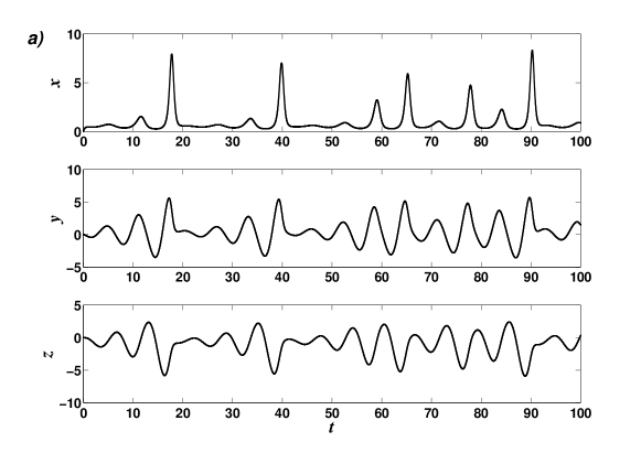
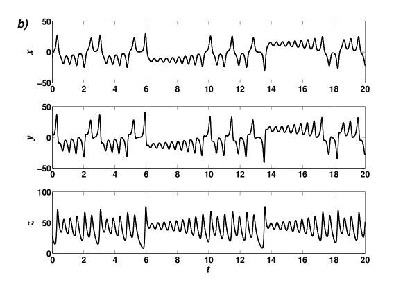
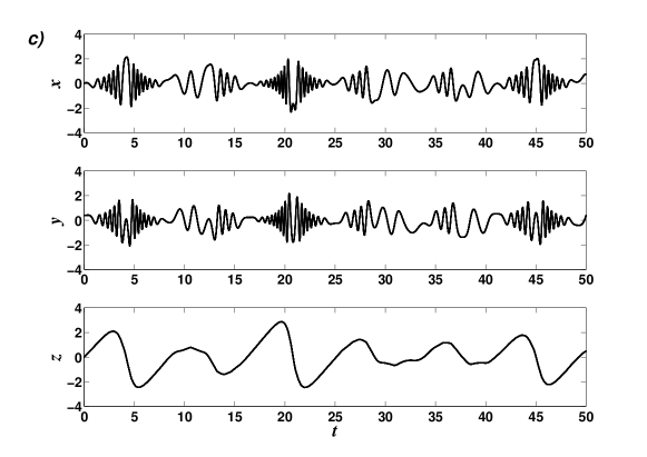
Figure 1: Evolution of the three coordinates as functions of time: (a) Rossler variables $x$, $y$, and $z$ for $\tau=0.01$ with $a=0.45$, $b=2$, and $c=4$. (b) Lorenz variables $x$, $y$, and $z$ for $\tau=0.001$ with $\sigma=16$, $r=45.92$, and $b=4$. (c) ${\mathbf{B}}_{7}$ variables $x$, $y$, and $z$ for $\tau=0.001$ with $K~{}=~{}0.5$, $\alpha~{}=~{}7.0$, and $\epsilon~{}=~{}0.23$.

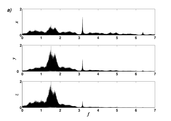
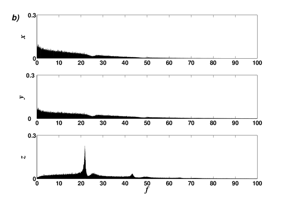
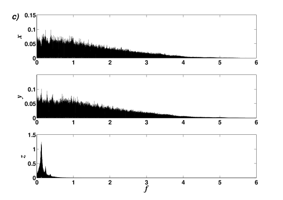
Figure 2: Power spectra of the coordinates $x$, $y$, and $z$ as a function of frequency: (a) Rossler System with $\tau=0.01$ with $a=0.45$, $b=2$, and $c=4$. for $\tau=0.01$, and $\Delta\tau=0.01$. (b) Lorenz System with $\sigma=16$, $r=45.92$, and $b=4$ for $\tau=0.001$, and $\Delta\tau=0.001$. (c) ${\mathbf{B}}_{7}$ System with $K~{}=~{}0.5$, $\alpha~{}=~{}7.0$, and $\epsilon~{}=~{}0.23$ for $\tau=0.001$, and $\Delta\tau=0.01$. In all the cases the time series length considered had $M=10^{5}~{}data$.

The first two systems exhibit strong differences that make them interesting for this study. The Rossler-oscillator “spends” most of the time near the plane $y,z$ with $x\simeq 0$. The time series obtained by sampling the $x$ coordinate looks like a delta train as Fig. 1.a illustrates. The Power Spectrum (PS) displayed in Fig. 2.a shows that the characteristic periodicities are very similar for all the three coordinates, with a higher frequency-content for $x$, produced by its delta like shape. On the other hand, the Lorenz oscillator displays a very different spectrum for coordinate $z$ (see Fig. 2.b), as compared with the PS of $x$ or $y$. The reason is that the attractor spirals from the center to the border of one of the typical butterfly’s wings and then suddenly moves to the other wing, as Fig. 1.b shows. Both attractors have correlation dimension $D_{2}$ close to $2$. The attractor ${\mathbf{B}}_{7}$ has a $D_{2}=2.719\pm 0.156$ [19], covering most of the available state-space. In Figs. 1.c and 2.c the time evolution of the three coordinates and their corresponding PS are displayed.

The evolution of each dynamical system was determined by recourse to a variable-step Runge-Kutta-Fehlberg approach [49]. Evaluations were made using sampling periods $\tau$ ranging from i) $0.01$ to $5$, in steps $\Delta\tau=0.01$ for the Rossler system, ii) $0.001$ to $0.3$ in steps of $\Delta\tau=0.001$ for the Lorenz system, and iii) $0.001$ to $1$ in steps of $\Delta\tau=0.001$ for ${\mathbf{B}}_{7}$ system. With these $\tau$’s one covers all the interesting regions: (1) the over-sampled one where $\tau$ is very small as compared with the characteristic times considered in Sec. 2 and 3, (2) the under-sampled region where $\tau$ is very large as compared with the characteristic times. For every $\tau-$value, $10$ realizations were generated by starting from different initial conditions. The time series for the state variables $x$, $y$, and $z$ were stored in a matrix of $3\;\times 10^{5}$, after skipping the first $10^{4}$ iterations in order that transient states die out.

We employed Bandt and Pompe’s procedure (with dimension $d=6$ and time lag $T=1$) to assign a PDF to each time series. These PDF’s exhibit an entropy $H^{(BP)}$ and a complexity $C^{(BP)}$. Functionals $H^{(hist)}$ and $C^{(hist)}$ were evaluated as well, with a PDF obtained from the pertinent histogram. In this case, the range covered by each variable was divided into $2^{16}$ uniformly distributed subintervals. The mean values $<C>$ and $<H>$ were computed for all the here considered PDF-functionals and all the realizations. For simplicity, the symbol $<\bullet>$, meaning mean value over realizations, is suppressed.

5.2 Our findings

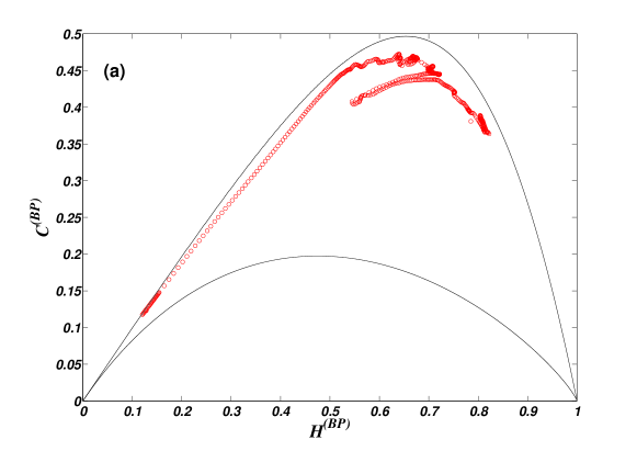
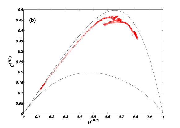
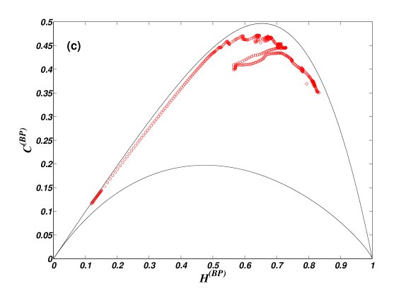
Figure 3: Representation on the entropy-complexity plane: (a-c) Rossler variables $x$, $y$, and $z$ for $0.01\leq\tau\leq 5$, $\Delta\tau=0.01$, with $a=0.45$, $b=2$, $c=4$. (d-f) Lorenz variables $x$, $y$, and $z$ for $0.001\leq\tau\leq 0.3$, $\Delta\tau=0.001$, with $\sigma=16$, $r=45.92$, and $b=4$. (g-i) ${\mathbf{B}}_{7}$ variables $x$, $y$, and $z$ for $0.001\leq\tau\leq 3$, $\Delta\tau=0.001$, with $K~{}=~{}0.5$, $\alpha~{}=~{}7.0$, and $\epsilon~{}=~{}0.23$. Undersampling corresponds to the high $H^{(BP)}$ and low $C^{(BP)}$ region, and oversampling to low $H^{(BP)}$ and low $C^{(BP)}$. In all the cases the time series length considered had $M=10^{5}~{}data$. The continuous lines represent, respectively, the maximum and minimum complexity values (for $d=6$) for a fixed value of the entropy.

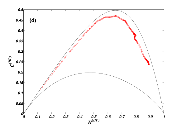
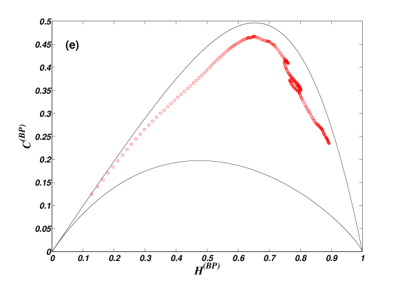
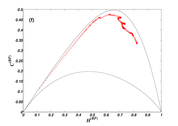
Figure 3: Continuation

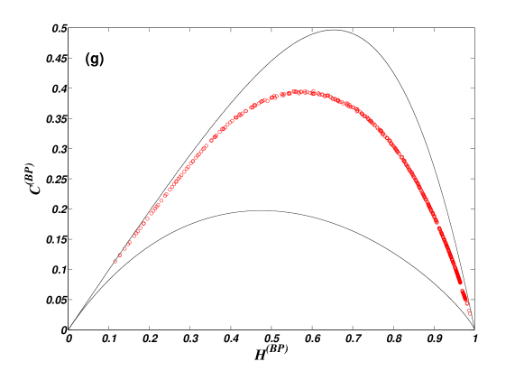
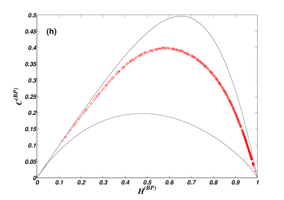
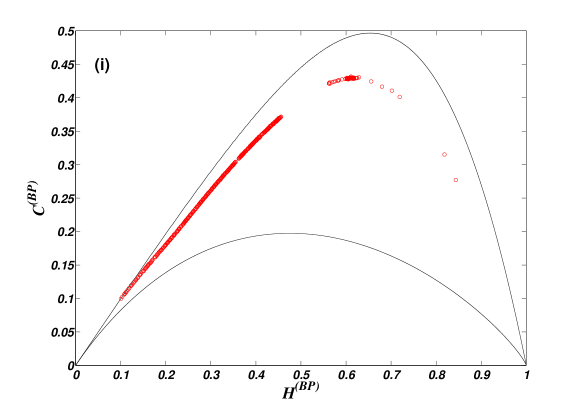
Figure 3: Continuation

The entropy-complexity plane $H^{(BP)}\times C^{(BP)}$ is quite useful for distinguishing between stochastic noise and deterministic chaotic behavior was recently illustrated in [6]. In such a vein we first analyze the planar evolution of representative points for our systems as the sampling frequency changes (see Fig. 3.a-c for the three sampled variables of the Rossler system, Fig. 3.d-f for the Lorenz system, and Fig. 3.g-i for the ${\mathbf{B}}_{7}$ system). As was explained in Sec. 4, “limiting curves” in the plots Fig. 3 determine the allowed values of entropy and complexity. There exists no PDF with entropy-complexity coordinates outside the region limited by these curves [25].

As the sample period $\tau$ decreases, the representative point evolves in the $H^{(BP)}\times C^{(BP)}$ plane, from the right planar region with low complexity and high entropy (under-sampling system with small sampling frequency $f=1/\tau$) to the left region with low complexity and low entropy (over-sampling with big sampling frequency $f=1/\tau$). The reason for such behavior is, as we comment in Sec. 2, that for a very big sampling period the dynamical correlations between consecutive measures are lost due to the mixing behavior of the chaotic system under study. That is, the measures can be completely uncorrelated and present characteristics like random behavior ($H\approx 1$ and $C\approx 0$). On the contrary, for very small sampling periods $\tau$ the measures will be (strongly) time-correlated so that successive measures suggest being in the presence of a very ordered system ($H\approx 0$ and $C\approx 0$). The evolution of the system in the $H^{(BP)}\times C^{(BP)}$ plane for regimes intermediate between these two extreme sampling-period instances will depend on the specific characteristics of the nonlinear system under study: whether it presents mixing or not; its chaos-degree, etc.

It is important to keep in mind that non linear correlations are the origin of the geometric structures that constitute the hallmark of deterministic chaos [6]. Precisely, in previous works $C^{(BP)}$ was seen to be a measure of the complexity induced by these non linear correlations. Our present results tell us that $f_{M}=1/t_{M}$ – the sampling frequency corresponding to the point with maximum complexity – can be regarded as the optimum sampling frequency, i.e, the minimum sampling frequency that retains all the information concerning these structures. Higher sampling frequencies imply an oversampling, producing unnecessary long files to cover the full attractor, while lower sampling frequencies make the time series to lose some vital information concerning nonlinear correlations. In the oversampled case, specific $d$-length ordinal patterns $(0,1,\cdots,d-1)$ and $(d-1,\cdots,1,0)$ appear more frequently than any other ordinal pattern, causing a low entropy $H^{(BP)}$ and a low complexity $C^{(BP)}$. Points in the region with high entropy and low complexity of the $H^{(BP)}\times C^{(BP)}$ plane correspond to undersampled trajectories of the continuous system. The samples are not correlated at all and the system behaves randomly. Consequently, all the ordinal patterns appear with almost the same frequency, as the ensuing high entropies $H^{(BP)}$ and low complexities $C^{(BP)}$ reveal. The evolution of the representative point in the plane $H^{(BP)}\times C^{(BP)}$ near the top limiting curve is typical of chaotic systems, as demonstrated by the authors of [6].

Let us stress the importance of using the Bandt and Pompe procedure to obtain the all-important PDF. A well-known result is that any chaotic map shares with its iterated maps the same histogram [50]. This property is the basis of the skipping randomizing technique [8, 51]. For that reason De Micco et al. [8] proposed the use of two different PDFs, as relevant for testing (i) the uniformity of $\mu(x)$ (the invariant measure) and (ii) the mixing constant $r_{mix}$ pertaining to a chaotic time series, as a means to generate pseudo random numbers. They proceeded to employ (a) a PDF $P_{1}$ based on time series’ histograms and (b) another PDF $P_{2}$ based on ordinal patterns (permutation ordering) that derives from appealing to the already cited Bandt and Pompe method [14]. One may conjecture that continuous systems exhibit an analogous property, viz., the sampling process does not significantly change the histogram of the time series and, consequently, any quantifier based on the PDF histogram is not sensitive to the sampling frequency.

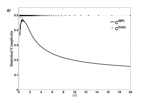
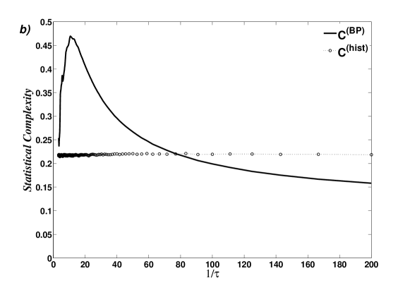
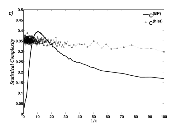
Figure 4: Intensive statistical complexity measures $C^{(BP)}$ and $C^{(hist)}$ for the coordinate $x$ of the three systems. (a) Rossler system, (b) Lorenz system and (c) ${\mathbf{B}}_{7}$ system one. $C^{(BP)}$ is evaluated by using the PDF obtained with the Bandt and Pompe prescription with $d=6$. $C^{(hist)}$ is evaluated by using the PDF obtained from the histogram of $x$, using $2^{16}$ bins. $C^{(hist)}$ is almost constant for all values of $\tau$. In all the cases the time series length considered had $M=10^{5}~{}data$. The use of the BP prescription is of the essence in getting the complexity-maxima. The reason is that a change in the sampling frequency does not change the invariant measure of each variable of the chaotic attractor. The situation is identical to that of the skipping procedure in pseudo random number generators based on chaotic maps [8].

Such conjecture is validated in Fig. 4, where the statistical complexities $C^{(BP)}$ and $C^{(hist)}$ are depicted as functions of the sampling frequency for the $x$-coordinates of the three systems (see Fig. 4.a for Rossler’s instance, Fig. 4.b for Lorenz’ case, and Fig. 4.c for ${\mathbf{B}}_{7}$). A similar result is obtained if $C^{(BP)}$ and $C^{(hist)}$ are evaluated for the other coordinates $y$ and $z$, and also if mean values $C^{(BP)}_{(xyz)}=[C^{(BP)}_{(x)}+C^{(BP)}_{(y)}+C^{(BP)}_{(z)}]/3$ and $C^{(hist)}_{(xyz)}=[C^{(hist)}_{(x)}+C^{(hist)}_{(y)}+C^{(hist)}_{(z)}]/3$ are used.

Consequently, we conclude that the usual histogram technique is not useful to analyze the effects of the sampling frequency and that a causal PDF (here the Bandt and Pompe one) must be employed instead. Note that in Figs. 3 and 4 many irregularities of the trajectories become visible. These are produced by the nontrivial relation between $C^{(BP)}$ and $H^{(BP)}$, and diminish as the number of realizations increases. Note that in Fig. 4, where $C^{(BP)}$ is represented as a function of $f=1/\tau$, a maximum is easily detected.

Table 1 summarizes our results. $t_{M}^{(x)}$, $t_{M}^{(y)}$, and $t_{M}^{(z)}$ are the inverses of the sampling frequency for each coordinate producing the maximum $C^{(BP)}$. We have evaluated $t_{M}^{(x)}$, $t_{M}^{(y)}$, and $t_{M}^{(z)}$ for each realization and then determined the associated mean values and standard deviations shown in columns $1$ to $6$. The mean value of $C^{(BP)}$ over coordinates $x$, $y$, and $z$ also exhibits a maximum for the $t_{M}$ indicated in column $7$ ($<x,y,z>$). All the characteristic times described in Sec. 2 and 3 are displayed in Table 1. Column $8$ displays the ratios between each characteristic time and the $t_{M}$ of column $7$. Figures closer to unity in column $8$ (within each class of characteristic times) are emphasized by using bold-types.

As we mention in Sec. 4, the normalized Shannon entropy and statistical complexity evaluated with PDF-Bandt and Pompe are not system invariant (neither are other quantifiers derived by Information Theory). The values of these quantifiers depend on how the PDF is evaluated. However, they provide very useful information about the dynamics of the system under study. It is clear then that $H^{(BP)}$ and $C^{(BP)}$ and the quantities derived from them could attain different values according with the specific time series considered (i.e. time series generated by the different coordinates of the system or a combination of them) even if it is reasonable to expect that their corresponding values do not exhibit a strong dispersion. This assumption is clearly confirmed if we look at the values obtained for $t_{M}$ in Table 1, evaluated for different times series. As expected, the same kind of behavior is obtained in the case of $t_{I}$ (Average Mutual Information).

From inspection of the results displayed in Tab. 1 we see that the time $t_{M}$ yields similar values to those obtained from the evaluation of the Average Mutual Information $t_{I}$. The largest difference between $t_{M}$ and $t_{I}$ (see column 8 in Tab. 1) is observed for the ${\mathbf{B}}_{7}$ system. Such disparity can be attributed to the fact that this system possesses an attractor with $D_{2}\approx 3$ (that covers most of the state-space) in contrast with the other two systems considered here, the Lorenz and Rossler ones, which have $D_{2}\approx 2$ [18, 24].

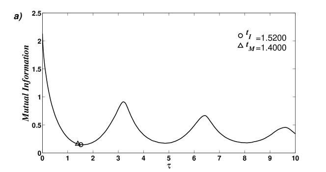
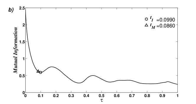
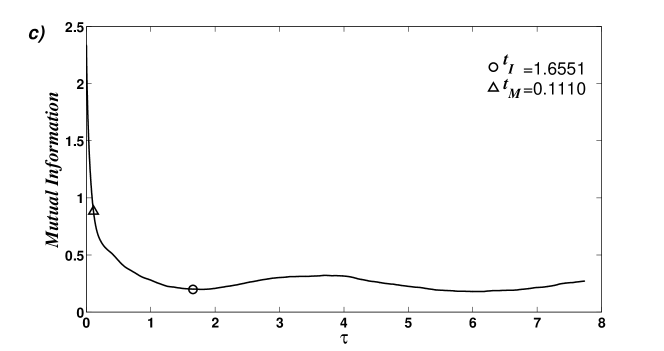
Figure 6: Discrete mutual information $I_{m}$ for: (a) Rossler System with $a=0.45$, $b=2$, $c=4$. (b) Lorenz System with $\sigma=16$, $r=45.92$, and $b=4$. (c) ${\mathbf{B}}_{7}$ System with $K~{}=~{}0.5$, $\alpha~{}=~{}7.0$ and $\epsilon~{}=~{}0.23$. In all the cases the time series length considered had $M=10^{5}~{}data$. The characteristic time induced by $C^{(BP)}$ ($d=6$), that is $t_{M}$ and its closest-lying characteristic time induced by $I_{m}$ are shown.

With regards to $t_{M}$ and the others special characteristic times (for our three dynamical systems) we can state that, in the Rossler-case, such characteristic times are, respectively, the first minimum of the mutual information $t_{3}$, the first zero of the autocorrelation $t_{0}$, and $t_{NS}$, for $\alpha=0.85$. In the the Lorenz-instance the characteristic times closest to $t_{M}$ are: the first minimum of the mutual information $t_{3}$, the first change of curvature of the autocorrelation $t_{2}$, and $t_{NS}$ for $\alpha=0.9$. Finally, for ${\mathbf{B}}_{7}$ the characteristic times closest to $t_{M}$ are: $t_{1/e}$, and $t_{NS}$ for $\alpha=0.85$. The first minimum of the mutual information appears far from the $t_{M}-$location. The shape of $I_{m}$ (discrete mutual information) is very irregular, as shown in Fig. 6.c, which explains why such features takes place.

For all the systems, the Nyquist criterion provides smaller characteristic times if $\alpha\geq 0.95$ is used instead, illustrating thus on the difference between the exact reconstruction that is the goal of the Nyquist-Shannon Theorem and the approximate attractor reconstruction that relies on Takens’ theorem. Note that the autocorrelation function is based just on linear statistics and does not contain any information concerning nonlinear dynamical correlations. Kantz and Schreiber [18] stressed the drawback of using linear statistics for the Lorenz system, with a typical trajectory staying some time on one wing of the butterfly attractor and spiralling then from the inside to the border before jumping to the other wing. The autocorrelation does not reveal the importance of the period of such “jumping” between wings, but the mutual information does so. Also, the autocorrelation of the squared signal is able to detect this periodic change [18].

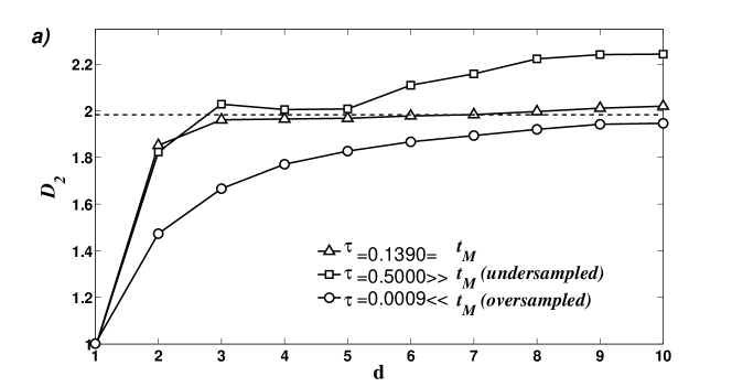
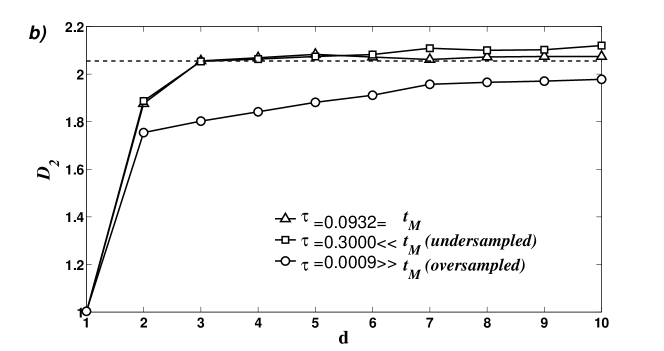
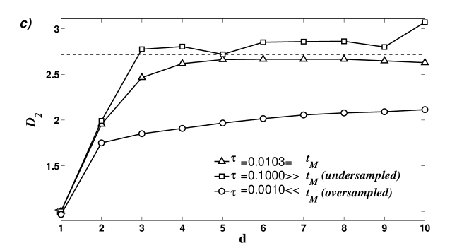
Figure 7: Mean value over realizations of the correlation dimension ($<D_{2}>$) for sampled $x$ ($y$ and $z$ samplings produce similar results) as a function of the embedding dimension $d$: (a) Rossler System with $a=0.45$, $b=2$, $c=4$. (b) Lorenz System with $\sigma=16$, $r=45.92$, and $b=4$. (c) ${\mathbf{B}}_{7}$ System with $K~{}=~{}0.5$, $\alpha~{}=~{}7.0$, and $\epsilon~{}=~{}0.23$. In all the cases the time series length considered had $M=10^{5}~{}data$. For oversampled series the value of $D_{2}$ remains below the reference value for any embedding dimension. For undersampled series all linear and nonlinear correlations are lost and the system behaves like a stochastic one. The correlation dimension $D_{2}$ increases with the embedding dimension $d$.

To assess the quality of the Takens’ reconstruction process using $t_{M}$, $D_{2}$ is evaluated for an embedding dimension ranging from $d=1$ to $10$ (see Fig. 7). The pertinent estimation of $D_{2}$ is compared with values reported in the literature for the continuous system [18, 52, 53]. The subroutine d2 of the TISEAN package [13] was used for calculating $D_{2}$.

Let us stress that the estimation of $D_{2}$ poses a very delicate problem, so that we refer the readers to the documentation available for the TISEAN package and also to the excellent book by Kantz and Schreiber [18]. Figs. 7 show that $\tau=t_{M}$ produces a time series with a $D_{2}$ that turns out to be a better estimation for the Correlation Dimension of the continuous system than those obtained with higher (under-sampled) or lower (over-sampled) values for $\tau$. Similar results were obtained when we consider the evaluation of the maximum Lyapunov exponent.

It is interesting to remark that the time $t_{M}$, for which one detects a maximum in the entropy-complexity plane $H^{(BP)}\times C^{(BP)}$, is unique for the three dynamical systems analyzed in the present work. We associate this sample-time with the one needed to capture all the relevant information related to the dynamics’ nonlinear correlations.

Recently Soriano et al. [20] theoretically and experimentally studied a chaotic semiconductor laser with optical feedback. This is an extremely interesting system because dynamical systems with time delay, like the Mackey-Glass or a laser with delay feedback, exhibit different relevant time scales [54, 20]. Consequently, additional complexity-maxima could be expected (in addition to the one encountered in dealing with the chaotic systems of this paper). In the case of the laser studied in [20] the main time scales are: i) $\tau^{*}_{S}$, the feedback-time providing the largest time scale, ii) $T_{RO}$, that is the relaxation oscillation providing a shorter time scale, and finally iii) chaotic oscillations, that govern the fastest time scale. Soriano et al. experimentally confirmed that our prescription for $t_{M}$ corresponds to a maximum of $C^{(BP)}$, as found in all the chaotic systems studied in this paper (see Fig. 10 in [20]). To our knowledge, this is the first controlled experiment where our prescription has been to hold.

Sharing the point of view of Abarbanel [24], our prescription for the sample period $\tau=t_{M}$ is based on the consideration of a fundamental aspect of chaos, namely, the generation of information. Thus, our choice is made by taking into account an important property of the system we wish to describe. Remark that stable linear systems generate zero information. In consequence, information-generation [24] is a property of nonlinear dynamics not shared by linear evolutions.

Finally, another issue to be aware of is the influence of noise. To verify the robustness of the criterion here advanced, gaussian noise was added to each system and the value of $t_{M}$ was obtained as a function of the signal to noise $S/N$ ratio ($\sigma$) of this gaussian noise. In all cases, the value of $t_{M}$ remained constant (up to three significant decimal digits) for $S/N>20~{}dB$. If the noise-strength is higher, $t_{M}$ suddenly decreases as the representative point in the plane $H^{(BP)}\times C^{(BP)}$ moves to the rightwards region (stochastic region), where ordering-patterns are strongly affected by noise.

6 Conclusions

Our main goal here was to show that a particular version of the Statistical Complexity Measure $C^{(BP)}$, evaluated by recourse to the probability distribution obtained via the Bandt and Pompe procedure, allows one to determine, under the light of a Takens’ reconstruction procedure, convenient sampling periods. This is done so as to get time series useful for investigating chaotic behavior.

This sampling-period was called $t_{M}$, and the procedure was illustrated via a detailed consideration of three paradigmatic systems. On the basis of these significant examples we conjecture that our optimality criterion may be of general application for chaotic systems, since $C^{(BP)}$ is a measure of the geometric structures produced by nonlinear correlations, always present in this class of dynamical systems. We showed that $t_{M}$ is compatible with those specific times recommended in the literature as adequate delay-ones in Takens’ reconstruction. Our results closely approach the exact Nyquist-Shannon reconstruction. This is so because high frequencies of the Fourier Spectrum are due to chaotic oscillations, and this is the case for the systems studied here.

To our knowledge, controlled experiments for different sampling times of the measured variables and large numbers of data have not yet been reported in the literature and the highest sampling frequency allowed by the digital acquisition system is the one usually adopted (as an exception see [20]). In the light of our present results it would be better, in practice, to assess the correct $t_{M}-$value for a clever choosing of the sampling period. This permits one to cover the whole attractor-basin and retain in the reconstruction process the most important properties of chaotic systems.

In view of the extensive use of digital acquisition systems in all kinds of experiments, we hope that experimentalists may consider the present contribution as a practical tool in their activities and may thus be able to validate our proposal.

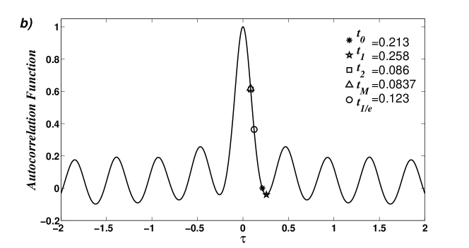
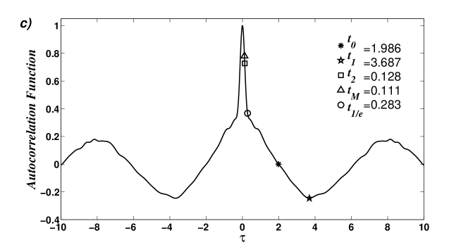
Figure 5: Discrete autocorrelation function $R_{m}$ for: (a) Rossler System with $a=0.45$, $b=2$, $c=4$. (b) Lorenz System with $\sigma=16$, $r=45.92$, and $b=4$. (c) ${\mathbf{B}}_{7}$ System with $K~{}=~{}0.5$, $\alpha~{}=~{}7.0$, and $\epsilon~{}=~{}0.23$. In all the cases the time series length considered had $M=10^{5}~{}data$. We show both the characteristic time induced by $C^{(BP)}$ ($d=6$), that is $t_{M}$, and its most approximate characteristic time induced by $R_{m}$.

Table 1: Characteristic Times for coordinates $x$, $y$, $z$ and their standard deviation (denoted by $\sigma_{i}$) of the Rossler, Lorenz and ${\mathbf{B}}_{7}$ chaotic attractors. System’s parameters are $a=0.45$, $b=2$, $c=4$ for Rossler, $\sigma=16$, $r=45.92$, and $b=4$ for Lorenz and $K=0.5$, $\alpha=7.0$, and $\epsilon=0.23$ for ${\mathbf{B}}_{7}$. In all the cases the time series length considered had $M=10^{5}~{}data$. $<x,y,z>$ represent the corresponding time obtained averaging $C^{(BP)}$ over the three coordinates. Each characteristic time is classified according with the method used to obtain it.Numbers in bold face indicate the characteristic time of each method that best approximates $t_{M}$ (the time corresponding to the maximum of the Statistical Complexity Measure $C^{(BP)}$ )($d=6$).

Rossler System
time	$x$	$\sigma_{x}$	$y$	$\sigma_{y}$	$z$	$\sigma_{z}$	$<x,y,z>$	$t/t_{M}$
Time induced by Complexity
$t_{M}$	1.3970	0.0067	1.8090	0.1473	1.4050	0.0053	1.4000	1.000
Times induced by Autocorrelation
$t_{0}$	1.4560	0.0178	1.5600	$<.00001$	1.7150	0.0118	1.6000	1.1429
$t_{1}$	3.2070	0.0157	3.0820	0.0063	3.2350	0.0108	3.1600	2.2571
$t_{2}$	0.6380	0.0079	1.3520	0.0103	1.5190	0.0032	1.0000	0.7143
$t_{1/e}$	0.8480	0.0157	1.1700	0.0063	1.2930	0.0108	1.1200	0.8000
Time induced by Mutual Information
$t_{I}$	1.6240	0.0534	1.4530	0.0874	1.5600	0.0337	1.5200	1.0857
Times induced by Nyquist-Shannon
$t_{NS}^{(0.85)}$	0.8795	–	1.4645	–	2.0956	–	1.4799	1.0571
$t_{NS}^{(0.90)}$	0.7292	–	1.1418	–	1.6661	–	1.1791	0.8422
$t_{NS}^{(0.95)}$	0.5691	–	0.7447	–	0.9142	–	0.7427	0.5305

Table 1: Continuation.

Lorenz System
time	$x$	$\sigma_{x}$	$y$	$\sigma_{y}$	$z$	$\sigma_{z}$	$<x,y,z>$	$t/t_{M}$
Time induced by Complexity
$t_{M}$	0.0932	0.0004	0.0722	0.0010	0.0853	0.0007	0.0860	1.0000
Times induced by Autocorrelation
$t_{0}$	2.3805	1.0482	1.9424	1.1457	0.1217	0.0018	0.2130	2.4767
$t_{1}$	0.4226	0.0308	0.3979	0.0342	0.2334	0.0007	0.2580	3.0000
$t_{2}$	0.1012	0.0006	0.0760	0.0001	0.0874	0.0005	0.0860	1.000
$t_{1/e}$	0.2078	0.0308	0.1478	0.0342	0.0883	0.0007	0.1230	14.3023
Time induced by Average Mutual Information
$t_{I}$	0.1048	0.0006	0.0970	0.0012	0.0941	0.0028	0.0990	1.1512
Times induced by Nyquist-Shannon
$t_{NS}^{(0.85)}$	0.1383	–	0.1082	–	0.0884	–	0.1116	1.2981
$t_{NS}^{(0.90)}$	0.1138	–	0.0880	–	0.0670	–	0.0896	1.0419
$t_{NS}^{(0.95)}$	0.0756	–	0.0639	–	0.0084	–	0.0493	0.5733

Table 1: Continuation.

${\mathbf{B}}_{7}$ System
time	$x$	$\sigma_{x}$	$y$	$\sigma_{y}$	$z$	$\sigma_{z}$	$<x,y,z>$	$t/t_{M}$
Time induced by Complexity
$t_{M}$	0.1030	$<0.001$	0.0930	$<0.001$	0.9540	$<0.001$	0.3833	1.0000
Times induced by Autocorrelation
$t_{0}$	0.5459	$0.3775$	0.5635	$0.4363$	1.9985	0.0258	1.9860	5.1808
$t_{1}$	0.4509	$0.1332$	0.3915	$0.0957$	3.9141	0.1161	3.6870	9.6182
$t_{2}$	0.1301	$0.0129$	0.1301	$0.0127$	1.5631	0.0227	0.1280	0.3339
$t_{1/e}$	0.1813	$0.1332$	0.1747	$0.0957$	1.4504	0.1161	0.2830	0.7382
Time induced by Average Mutual Information
$t_{I}$	1.5289	0.2240	1.5951	0.2212	1.7905	0.1041	1.6551	4.3176
Times induced by Nyquist-Shannon
$t_{NS}^{(0.85)}$	0.1901	–	0.1968	–	0.5319	–	0.3062	0.7987
$t_{NS}^{(0.90)}$	0.1683	–	0.1736	–	0.0731	–	0.1383	0.3607
$t_{NS}^{(0.95)}$	0.0539	–	0.1441	–	0.0076	–	0.06853	0.1787

References

- [1] J. P. Crutchfield, K. Young. Inferring statistical complexity. Phys. Rev. Lett. 63 (1989) 105–108.
- [2] R. Wackerbauer, A. Witt, H. Atmanspacher, J. Kurths, H. Scheingraber. A comparative classification of complexity measures. Chaos, Solitons & Fractals, 4 (1994) 133–173.
- [3] R. López-Ruiz, H. L. Mancini, X. Calbet. A statistical measure of complexity. Phys. Lett. A 209 (1995) 321–326.
- [4] M. T. Martín, A. Plastino, and O. A. Rosso. Statistical complexity and disequilibrium. Phys. Lett. A 11 (2003) 126–132.
- [5] P. W. Lamberti, M. T. Martín, A. Plastino, and O. A. Rosso. Intensive entropic non-triviality measure. Physica A 334 (2004) 119–131.
- [6] O. A. Rosso, H. A. Larrondo, M. T. Martín, A. Plastino, M. A. Fuentes. Distinguishing noise from chaos. Phys. Rev. Lett. 99 (2007) 154102.
- [7] O. A. Rosso, L. Zunino, D. G. Pérez, A. Figliola, H. A. Larrondo, M. Garavaglia, M. T. Martín, A. Plastino. Extracting features of gaussian selfsimilar stochastic processes via the Bandt & Pompe approach. Phys. Rev. E, 76 (2007) 061114.
- [8] L. De Micco, C. M. González, H. A. Larrondo, M. T. Martín, A. Plastino, O. A. Rosso. Randomizing nonlinear maps via symbolic dynamics. Physica A 387 (2008) 3373–3383.
- [9] L. De Micco, H. Larrondo, A. Plastino, O. A. Rosso. Quantifiers for stochasticity of chaotic pseudo random number generators. Phil. Trans. Royal Soc. A 367 (2009) 3281–3296.
- [10] H. Nyquist. Certain topics in telegraph transmission theory. Trans. AIEE 47 (1928) 617–644.
- [11] C. E. Shannon. Communication in the presence of noise. Proc. Institute of Radio Engineers 37 (1949) 10–21.
- [12] F. Takens. Detecting strange attractors in turbulence. Lecture Notes in Mathematics 898 (1981) 366–381.
- [13] R. Hegger, H. Kantz, and T. Schreiber. Practical implementation of nonlinear time series methods: The tisean package. Chaos 9 (1999) 413–435.
- [14] C. Bandt, B. Pompe. Permutation entropy: a natural complexity measure for time series. Phys. Rev. Lett. 88 (2002) 174102.
- [15] J. Pearl. Causality: models, reasoning, and inference. Cambridge University Press, 2009.
- [16] A. M. Fraser, H. L. Swinney. Independent coordinates for strange attractors from mutual information. Phys. Rev. A 33 (1986) 1134–1140.
- [17] J. P. Crutchfield, B. McNamara. Equations of motion from a data series. Complex Systems 1 (1989) 417–452.
- [18] H. Kantz, T. Shreiber. Nonlinear Time Series Analysis. Cambridge University Press, 1999.
- [19] K. E. Chlouverakis and J. C. Sprott. A comparison of correlation and lyapunov dimensions. Physica D 200 (2005) 156–164.
- [20] M. C. Soriano, L. Zunino, O. A. Rosso, I. Fischer, C. R. Mirasso. Time scales of chaotic semiconductor laser with optical feedback under the lens of permutation information analysis. IEEE J. Quantum Electronics 47 (2011) 252–261.
- [21] T. Sauer, J. A. Yorke, M. Casdagli. Embedology. Journal of Statistical Physics 65 (1991) 579–616.
- [22] M. Casdagli, S. Eubank, J. D. Farmer, J. Gibson. State space reconstruction in the presence of noise. Physica D 51 (1991) 52–98.
- [23] J. Gibson, J. D. Farmer, M. Casdagli, S. Eubank. An analytical approach to practical state space reconstruction. Physica D 57 (1992) 1–30.
- [24] H. D. I. Abarbanel. Analysis of observed chaotic data. Springer-Verlag, New York, 1996.
- [25] M. T. Martín, A. Plastino, O. A. Rosso. Generalized statistical complexity measures: geometrical and analytical properties. Physica A 369 (2006) 439–462.
- [26] O. A. Rosso, H. Craig, P. Moscato, Shakespeare and other English renaissance authors as characterized by Information Theory complexity quantifiers. Physica A 388 (2009) 916–926
- [27] K. Mischaikow, M. Mrozek, J. Reiss, A. Szymczak. Construction of symbolic dynamics from experimental time series. Phys. Rev. Lett., 82 (1999) 1114–1147.
- [28] G. E. Powell, I. C. Percival. A spectral entropy method for distinguishing regular and irregular motion of hamiltonian systems. J. Phys. A: Math. Gen. 12 (1979) 2053–2071.
- [29] S. Blanco, A. Figliola, R. Quian Quiroga, O. A. Rosso, E. Serrano. Time-frequency analysis of electroencephalogram series (III): Wavelet packets and information cost function. Phys. Rev. E 57 (1998) 932–940.
- [30] O. A. Rosso, S. Blanco, J. Jordanova, V. Kolev, A. Figliola, M. Schürmann, E. Başsar. Wavelet entropy: a new tool for analysis of short duration brain electrical signals. Journal of Neuroscience Methods 105 (2001) 65–75.
- [31] W. Ebeling, R. Steuer. Partition-based entropies of deterministic and stochastic maps. Stochastics and Dynamics, 1 (2001) 1–17.
- [32] J. M. Amigó, L. Kocarev, I. Tomovski. Discrete entropy. Physica D 228 (2007) 77–85.
- [33] K. Keller, M. Sinn. Ordinal analysis of time series. Physica A 356 (2005) 114–120.
- [34] O. A. Rosso, C. Masoller. Detecting and quantifying stochastic and coherence resonances via information theory complexity measurements. Phys. Rev. E 79 (2009) 040106(R).
- [35] O. A. Rosso, C. Masoller. Detecting and quantifying temporal correlations in stochastic resonance via information theory measures. European Phys. Journal B, 69 (2009) 37–43.
- [36] H. A. Larrondo, C. M. González, M. T. Martín, A. Plastino, O. A. Rosso. Intensive statistical complexity measure of pseudorandom number generators. Physica A 356 (2005) 133–138.
- [37] H. A. Larrondo, M. T. Martín, C.M. González, A. Plastino, O. A. Rosso. Random number generators and causality. Phys. Lett. A 352 (2006) 421–425.
- [38] A. M. Kowalski, M. T. Martín, A. Plastino, O. A. Rosso. Bandt-Pompe approach to the classical-quantum transition. Physica D 233 (2007) 21–31.
- [39] L. Zunino, D. G. Pérez, M. T. Martín, A. Plastino, M. Garavaglia, O. A. Rosso. Characterization of gaussian self-similar stochastic processes using wavelet-based informational tools. Phys. Rev. E 75 (2007) 021115.
- [40] O. A. Rosso, R. Vicente, C. R. Mirasso. Encryption test of pseudo-aleatory messages embedded on chaotic laser signals: an information theory approach. Phys. Lett. A 372 (2008) 1018–1023.
- [41] L. Zunino, D. G. Pérez, M. T. Martín, M. Garavaglia, A. Plastino, O. A. Rosso. Permutation entropy of fractional brownian motion and fractional gaussian noise. Physics Letters A 372 (2008) 4768–4774.
- [42] L. Zunino, D. G. Pérez, A. Kowalski, M. T. Martín, M. Garavaglia, A. Plastino, O. A. Rosso. Fractional Brownian motion, fractional Gaussian noise, and Tsallis permutation entropy. Physica A 387 (2008) 6057–6068
- [43] L. Zunino, M. Zanin, B. M. Tabak, D. Perez, and O. A. Rosso. Forbidden patterns, permutation entropy and stock market inefficiency. Physica A 388 (2009) 2854–2864
- [44] L. Zunino, M. Zanin, B. M. Tabak, D. G. Pérez, O. A. Rosso. Complexity-entropy causality plane: a useful approach to quantify the stock market inefficiency. Physica A 389 (2010) 1891–1901.
- [45] O. A. Rosso, L. De Micco, H. Larrondo, M. T. Martín, A. Plastino. Generalized statistical complexity measure. Int. J. Bif. and Chaos 20 (2010) 775–785.
- [46] O. A. Rosso, L. De Micco, A. Plastino, H. A. Larrondo. Info-quantifiers’ map-characterization revisited. Physica A 389 (2010) 4604–4612.
- [47] P. M. Saco, L. C. Carpi, A. Figliola, E. Serrano, and O. A. Rosso. Entropy Analysis of the Dynamics of EL Niño/Southern Oscillation during the Holocene. Physica A 389 (2010) 5022–5027.
- [48] K. Keller, H. Lauffer. Symbolic analysis of high-dimensional time series. Int. J. Bifurcation and Chaos 13 (2003) 2657–2668.
- [49] W. H. Press, S. A. Teikolsky, W. T. Vetterling, B. P. Flannery. Numerical Recipes in C. Cambridge University Press, 1995.
- [50] G. Setti, G. Mazzini, R. Rovatti, and S. Callegari. Statistical modeling of discrete-time chaotic processes: Basic finite-dimensional tools and applications. Proceedings of the IEEE 90 (2002) 662–689.
- [51] S. Callegari, R. Rovatti, and G. Setti. Chaos-based fm signals: application and implementation issues. IEEE Transactions on Circuits and Systems I: Fundamental Theory and Applications 50 (2003) 1141–1147.
- [52] J. C. Sprott. Lyapunov exponent and dimension of the lorenz attractor. http://sprott.physics.wisc.edu/chaos/lorenzle.htm, 2005.
- [53] J. C. Sprott, C. Rowlands. Improved correlation dimension calculation. Int. J. Bifurcation and Chaos 11 (2001) 1865–1880.
- [54] L. Zunino, M. C. Soriano, I. Fischer, O. A. Rosso, C. R. Mirasso. Permutation-information-theory approach to unveil delay dynamics from time-series analysis. Phys. Rev. E 82 (2010) 046212.