The emergence of Special and Doubly Special Relativity

Abstract

Abstract

Building on our previous work [Phys. Rev. D82, 085016 (2010)], we show in this paper how a Brownian motion on a short scale can originate a relativistic motion on scales that are larger than particle’s Compton wavelength. This can be described in terms of polycrystalline vacuum. Viewed in this way, special relativity is not a primitive concept, but rather it statistically emerges when a coarse graining average over distances of order, or longer than the Compton wavelength is taken. By analyzing the robustness of such a special relativity under small variations in the polycrystalline grain-size distribution we naturally arrive at the notion of doubly-special relativistic dynamics. In this way, a previously unsuspected, common statistical origin of the two frameworks is brought to light. Salient issues such as the rôle of gauge fixing in emergent relativity, generalized commutation relations, Hausdorff dimensions of representative path-integral trajectories and a connection with Feynman chessboard model are also discussed.

I Introduction 

Without doubts the discovery of Lorentz symmetry (LS) irrevocably changed the theoretical landscape in physics. Up to now LS has been confirmed to unprecedent precision, and during the last century it has powerfully constrained theories in a way that has proved instrumental in discovering new laws of physics. Moreover, the mathematical structure of the Lorentz group is compellingly simple and elegant. It thus seems natural to assume that Lorentz invariance is an exact symmetry of nature which is valid for an arbitrary boost. Yet, there are several reasons to doubt the exactness of LS. From a purely conceptual standpoint, the most cogent reason is that an infinite volume of the Lorentz group is experimentally untestable since, unlike the rotation group, the Lorentz group is non-compact. Why should one then assume that exact LS holds when this hypothesis cannot be tested, not even in principle? The non-compactness may, indeed, sound as a logically convincing argument for doubting the exactness of LS but in itself is not enough to attract a sufficient attention. There are, however, other more pressing reasons to suspect that LS may fail at some critical energy or boost. For instance, in quantum field theory both the ultraviolet divergences and Landau poles are direct artifacts of the assumption that the spectrum of field degrees of freedom is boost invariant. Another sound reason comes from quantum gravity where profound difficulties associated with the problem of time Isham ; Isham II ; Kuchar indicate that an underlying preferred time may be necessary in order to reconcile gravitational and quantum physics. In particular, general arguments imply that a radical departure from standard space-time symmetries at the Planck scale thooft-a is necessary. Aside from general issues of principle, specific hints of Lorentz violation come from tentative calculations in various approaches to quantum gravity. Examples include: space-time foam hawking , cosmologically varying moduli Damour , Witten’s string field theory Kostelecky II , semiclassical spin-network calculations in Loop quantum gravity Gambini ; Alfaro , non-commutative geometry Hayakawa ; Carrol ; Anisimov , world-crystal physics HKII ; JKS1 , ’t Hooft’s cosmic cellular automata thooft or condensed matter analogues of emergent gravity Volovik03 . None of the above reasons amount to a convincing argument that a LS breaking is an inevitable aspect of quantum gravity. However, taken together they do motivate serious attempts to address possible observable consequences of a violation of LS, and to strengthen observational bounds. What should be perhaps emphasized is that the idea of LS violation is not new and it has been considered by a number of authors over the last forty years or so (see, e.g. Refs. fock ; DSR and citations therein). It has, however, received a serious boost only during the past decade. The catalyst has been both a massive infusion of ideas from quantum gravity, and improvements in observational sensitivity that allow to detect violations of LS that are linearly Planck suppressed (see e.g., jacobson:08 for an extensive review).

In this paper we show that a relativistic quantum mechanics, as formulated through path integrals (PI), bears in itself a seed of understanding how LS can be broken at short spatio-temporal scales and yet emerge as an apparently exact symmetry at large scales. Our argument is based upon a recent observation JK1 ; JK2 that PI for both fermionic and bosonic relativistic particles may be interpreted (when analytically continued to imaginary times) as describing a doubly-stochastic process that operates on two vastly different spatio-temporal scales. The short spatial scale, which is much smaller than the Compton length, describes a Wiener (i.e., non-relativistic) process with a fluctuating Newtonian mass. This might be visualized as if the particle would be randomly propagating (in the sense of Brownian motion) through a granular or “polycrystalline” medium. The large spatial scale corresponds, on the other hand, to distances that are much larger than particle’s Compton length. At such a scale the particle evolves according to a genuine relativistic motion, with a sharp value of the mass coinciding with the Einstein rest mass. Particularly striking is the fact that when we average the particle’s velocity over the correlation distance (i.e., over particle’s Compton wavelength) we obtain the velocity of light $c$. So the picture that emerges from this analysis is that the particle (with a non-zero mass!) propagates over the correlation distance $~{}1/mc$ (hereafter $\hbar=1$) with an average velocity $c$, while at larger distance scales (i.e., when a more coarse grained view is taken) the particle propagates as a relativistic particle with a sharp mass and an average velocity that is smaller than $c$. This bears a strong resemblance with Feynman’s chessboard PI for a relativistic Dirac fermion in $1+1$ dimensions FH . There, an analogous situation occurs, i.e., a massive particle propagates over distances of Compton length with velocity $c$, and it is only on much larger spatial scales where the Brownian motion with a sub-luminal average velocity emerges FH ; Schulman-Jacobson . The analogy with Feynman’s chessboard PI appears also on the level of Hausdorff dimensions of representative trajectories. While below the Compton wavelength the Haussdorff dimension $d_{H}=1$, which corresponds to a super-diffusive process, on scales much larger than the Compton length one has $d_{H}=2$, which is the usual Brownian diffusion. In passing, we may stress that the outlined superposition of two stochastic processes with widely separated times scales fits the conceptual framework which is often referred to as a superstatistics Beck:01 .

Of course, a single-particle relativistic quantum theory is a logically untenable concept, since a multi-particle production is allowed whenever the particle reaches the threshold energy for pair production. At the same time, the PI for a single relativistic particle is a perfectly legitimate building block in quantum field theory (QFT). Indeed, QFT can be viewed as a grand-canonical ensemble of particle histories where Feynman diagrammatic representation of quantum fields depicts directly the pictures of the world-lines in a grand-canonical ensemble. In particular, the partition function for quantized relativistic fields can be fully rephrased in terms of single-particle relativistic PI’s. This view is epitomized, e.g., in the Bern–Kosower “string-inspired” approach to quantum field theory Bern-Kosower or in Kleinert’s disorder field theory KleinertIII .

The outlined scenario can be also conveniently applied in various doubly special relativistic (DSR) models. In those models a further invariant scale $\ell$, besides the speed of light $c$, is introduced, and $\ell$ is assumed typically to be of the order of the Planck length. In the present framework, the scale $\ell$ can be naturally identified with the minimal grain size of the polycrystalline medium. By following the same strategy as in the special relativistic context, i.e., analyzing the structure of paths which enter the Feynman summation, one can again identify correlation lengths, canonical commutation relations and the respective Hausdorff dimensions. All of these critically depend on the DSR model at hand, and may serve to gain insight into the underlying stochastic process which is, as a rule, related by an analytic continuation with the corresponding quantum mechanical dynamics.

The purpose of this paper is to call attention to such a peculiar behavior of relativistic PI at short spatio-temporal scales — a fact already recognized by Feynman — and bring ensuing implications to the attention of our particle-physics and cosmology colleagues.

The structure of the paper is as follows. To set the stage we recall in the next section some fundamentals of Markovian smearing of path integrals, also known as superstatistics path integrals (SPI). Section III is devoted to application of SPI in relativistic quantum mechanics. We restrict our presentation largely to bosons of zero spin that are described by the Klein–Gordon equation. Thought the Klein–Gordon particle (KGP) is not a key for the results obtained, it will allow to elucidate the physics behind our reasonings quite straightforwardly. In particular we show how a transitional amplitude for the KGP can be written as a superposition of non-relativistic free-particle PI’s with different Newtonian masses. To this end we use a less known but equivalent representation of Klein–Gordon equation, namely the so-called Feshbach–Villars representation. The concept of emergent relativity is discussed in Section IV. There we observe that the superstatistics version of Feynman path summation for a relativistic particle allows the following probabilistic interpretation: the single-particle relativistic theory might be viewed as a single-particle non-relativistic theory (Wiener process) whose Newtonian mass $\tilde{m}$ (which is not invariant under Lorentz transformations) is a fluctuating parameter, whose average approaches the true relativistic Einstein mass $m$ at observational (or resolution) times that are much larger than the Compton time $1/mc^{2}$. On a spatial scale greater than the particle’s Compton wave length the particle follows the standard relativistic motion with a sharp mass and a sub-luminal average velocity. Sections V and VI contain discussions of two conceptually important concomitant topics. In particular, Section V concentrate on the issue of stability of the emergent special relativity (SR) under a small perturbation of the grain (or mass-smearing) distribution in the polycrystalline vacuum. There we show that small perturbations naturally lead to the DSR theory. Hence the class of DSR models (of which the special relativity theory is a particular example) is robust under and a small change of the grain-size distribution. In Section VI, we are concerned with the question of how a choice of a gauge fixing influences our polycrystalline-vacuum picture. We employ the Stückelberg field-enlarging trick and show that the SPI in question can be made explicitly invariant under gauge transformations (or reparametrizations), i.e., under the same group under which relativistic particle systems are invariant. By revealing that our original action is dynamically equivalent to the relativistic action with the reparametrization symmetry we are allowed to proclaim the “polycrystalline” picture as being a basic (or primitive) edifice of SR, and consider the reparametrization symmetry as a mere artifact of an artificial redundancy that is allowed in the description.

In Section VII, we extend our approach to doubly special relativistic dynamics, sketch the computation of the ensuing canonical commutation relations (CCR’s) and the Hausdorff dimensions of representative trajectories. Since the smearing distribution implicitly corresponds to the gauge fixing condition, the obtained CCR automatically match the quantized Dirac brackets. It is, indeed, a bonus of the superstatistics PI for (doubly-)relativistic particle that it directly provides a symplectic structure in the reduced phase space. We close Section VII with some comments on the underlying non-relativistic picture.

Various remarks and generalizations are proposed in the concluding section. For the reader’s convenience the paper is supplemented with four appendices which clarify some finer technical details.

II Superstatistics path integrals

We begin with the well known fact that when a conditional probability density functions (PDF’s) is formulated through PI then it satisfies the Chapman–Kolmogorov equation (CKE) for continuous Markovian processes, namely

$$P(x_{b},t_{b}|x_{a},t_{a})=\int_{-\infty}^{\infty}{\rm{d}}x\ \!P(x_{b},t_{b}|x,t)P(x,t|x_{a},t_{a})\,.$$ (1)

Conversely, any probability satisfying CKE possesses a PI representation FH ; Kac .

In physics one often encounters probabilities formulated as a superposition of PI’s, e.g.

$$\mbox{}\bar{P}(x_{b},t_{b}|x_{a},t_{a})$$

$$\mbox{}=\!\int_{0}^{\infty}{\rm{d}}v\ \omega(v,t_{ba})\int_{x(t_{a})=x_{a}}^{x(t_{b})=x_{b}}{\mathcal{D}}x{\mathcal{D}}p\ e^{\int_{t_{a}}^{t_{b}}{\rm{d}}\tau\left(\footnotesize{{\rm{i}}}p\dot{x}-vH(p,x)\right)}\,.$$

(2)

Here $\omega(v,t_{ba})$ with $t_{ba}=t_{b}-t_{a}$ is a normalized PDF defined on ${\mathbb{{R}}}^{+}\!\!\times{\mathbb{{R}}}^{+}$. The random variable $v$ is in practice typically related to the inverse temperature, coupling constant, friction constant or volatility.

At this stage one may ask if is it possible that also $\bar{P}({{\mbox{\boldmath{$x$}}}}_{b},t_{b}|{{\mbox{\boldmath{$x$}}}}_{a},t_{a})$ satisfies the CKE (1). The answer is surprisingly affirmative provided $\omega(v,t)$ fulfills a certain simple functional equation. Following Ref. JK1 we define a rescaled weight function

$$w(v,t)\ \equiv\ \omega(v/t,t)/t\,,$$ (3)

and calculate its Laplace transform

$$\tilde{w}(p_{v},t)\ \equiv\ \int_{0}^{\infty}{\rm{d}}v\ \!e^{-p_{v}v}w(v,t)\,.$$ (4)

Then $\bar{P}({{\mbox{\boldmath{$x$}}}}_{b},t_{b}|{{\mbox{\boldmath{$x$}}}}_{a},t_{a})$ satisfies CKE only if

$$\tilde{w}(p_{v},t_{1}+t_{2})\ =\ \tilde{w}(p_{v},t_{2})\tilde{w}(p_{v},t_{1})\,.$$ (5)

Assuming continuity in $t$, $w(p_{v},t)$ is unique and can be explicitly written as (see JK1 ):

$$\tilde{w}(p_{v},t)\ =\ [G(p_{v})]^{t}\ =\ e^{-tF(p_{v})}\,.$$ (6)

A function $F(p_{v})$ must increase monotonically in order to allow for inverse Laplace transform, and satisfy the condition $F(0)=0$ to ensure that $\omega$ is normalized to one. Finally the Laplace inverse of $\tilde{w}(p_{v},t)$ yields $\omega(v,t)$.

Once the above conditions are satisfied, then $\bar{P}({{\mbox{\boldmath{$x$}}}}_{b},t_{b}|{{\mbox{\boldmath{$x$}}}}_{a},t_{a})$ possesses a path integral representation on its own. The new Hamiltonian is given by the relation $\bar{{H}}({{\mbox{\boldmath{$p$}}}},{{\mbox{\boldmath{$x$}}}})=F(H({{\mbox{\boldmath{$p$}}}},{{\mbox{\boldmath{$x$}}}}))$. Here one must worry about the notorious operator-ordering problem, not knowing in which temporal order $p$ and $x$ must be taken in $F$. At this stage it suffices to observe that when $H$ is $x$ independent, the former relation is exact. The issue of general $H$’s and the ensuing operator ordering was discussed in detail in Ref. JK1 .

III Path integral for Feshbach–Villars particle

Our following argument is based upon Refs. JK1 ; JK2 where it was shown that the Newton–Wigner NW ; HK propagator for a relativistic scalar particle with Hamiltonian $\hat{H}({{\mbox{\boldmath{$p$}}}})=c\sqrt{\hat{{\mbox{\boldmath{$p$}}}}^{2}+m^{2}c^{2}}$, i.e.

$$P({{\mbox{\boldmath{$x$}}}}_{b},t_{b}|{{\mbox{\boldmath{$x$}}}}_{a},t_{a})\ =\ \int_{\footnotesize{{\mbox{\boldmath{$x$}}}}(t_{a})\ \!=\ \!\footnotesize{{\mbox{\boldmath{$x$}}}}_{a}}^{\footnotesize{{\mbox{\boldmath{$x$}}}}(t_{b})\ \!=\ \!\footnotesize{{\mbox{\boldmath{$x$}}}}_{b}}{\mathcal{D}}{{\mbox{\boldmath{$x$}}}}\frac{\mathcal{D}{{\mbox{\boldmath{$p$}}}}}{(2\pi)^{D}}\ \!\exp\left\{\int_{t_{a}}^{t_{b}}\!\!{\rm{d}}\tau\ \!\left[{\rm{i}}{{\mbox{\boldmath{$p$}}}}\cdot\dot{{\mbox{\boldmath{$x$}}}}-c\sqrt{{{\mbox{\boldmath{$p$}}}}^{2}+m^{2}c^{2}}\right]\right\}\,,$$ (7)

can be considered as a superposition of non-relativistic free-particle path integrals provided one chooses the generating function $G(p_{v})\ =\ e^{-a\sqrt{p_{v}}}$ with $a\in\mathbb{{R}}^{+}$. In such a case one obtains JK1 ; JK2

$$P({{\mbox{\boldmath{$x$}}}}_{b},t_{b}|{{\mbox{\boldmath{$x$}}}}_{a},t_{a})\ =\ \int_{0}^{\infty}\!\!\!{\rm{d}}v\ \!\omega(v,t_{ba})\int_{\footnotesize{{\mbox{\boldmath{$x$}}}}(t_{a})\ \!=\ \!\footnotesize{{\mbox{\boldmath{$x$}}}}_{a}}^{\footnotesize{{\mbox{\boldmath{$x$}}}}(t_{b})\ \!=\ \!\footnotesize{{\mbox{\boldmath{$x$}}}}_{b}}{\mathcal{D}}{{\mbox{\boldmath{$x$}}}}\ \!\frac{\mathcal{D}{{\mbox{\boldmath{$p$}}}}}{(2\pi)^{D}}\ \!\exp\left\{\int_{t_{a}}^{t_{b}}\!\!\!{\rm{d}}\tau\ \![{\rm{i}}{{\mbox{\boldmath{$p$}}}}\cdot\dot{{\mbox{\boldmath{$x$}}}}-v({{\mbox{\boldmath{$p$}}}}^{2}c^{2}+m^{2}c^{4})]\right\}\,,$$ (8)

with $\omega(v,t)$ being the Weibull distribution of order $1$. In general, Weibull’s PDF of order $a$ is defined as weibull

$$\omega(v,a,t)\ =\ \frac{a\exp\left(-a^{2}t/4v\right)}{2\sqrt{\pi}\sqrt{v^{3}/t}}\,.$$ (9)

We note that, neither (7) nor (8) are propagators for Klein–Gordon equation. As stressed first by Stuckelberg Stuckelberg:41 ; Stuckelberg:42 , the true relativistic propagator must include also the negative energy spectrum, reflecting the existence of charge-conjugated solutions, i.e., antiparticles.

Recently, it was pointed out that the resolution of this problem in the framework of PI’s can be readily found when the Klein–Gordon particle is written in the so-called Feshbach–Villars (FV) representation JK2

$$i\partial_{t}\Psi\ =\ \hat{H}_{{}_{\rm FV}}({{\mbox{\boldmath{$p$}}}})\Psi\,,$$

$$\hat{H}_{{}_{\rm FV}}({{\mbox{\boldmath{$p$}}}})\ =\ (\sigma_{3}+{\rm{i}}\sigma_{2})\frac{\hat{{\mbox{\boldmath{$p$}}}}^{2}}{2m}\ +\ \sigma_{3}mc^{2}\,,$$ (10)

where $\Psi$ is a two component wave function. The two components are related to opposite parity states — fact that is automatically fulfilled by Dirac bispinors in case of Dirac’s equations. FV representation was already thoroughly discussed in Ref. JK2 and we shall refrain from going to further details here. The interested reader is referred to Appendix A where the relevant essentials are presented. Here we only mention that in order to deal with the full PI representation of the Klein–Gordon particle it will suffice to discuss the PI relation (8) alone, see Eq. (Appendix A).

IV Emergent Special Relativity

If we now consider the change of variable $vc^{2}\leftrightarrow 1/2\tilde{m}$, then the RHS of the key relativistic PI identity (8) can be rewritten in the form [see also Ref. JK2 ]

$$\mbox{}\int_{\footnotesize{{\mbox{\boldmath{$x$}}}}(0)\ \!=\ \!\footnotesize{{\mbox{\boldmath{$x$}}}}^{\prime}}^{\footnotesize{{\mbox{\boldmath{$x$}}}}(t)\ \!=\ \!\footnotesize{{\mbox{\boldmath{$x$}}}}}\ \!{\mathcal{D}}{{\mbox{\boldmath{$x$}}}}\frac{\mathcal{D}{{\mbox{\boldmath{$p$}}}}}{(2\pi)^{D}}\ \!\exp\left\{\int_{0}^{t}\!\!{\rm{d}}\tau\ \!\left[{\rm{i}}{{\mbox{\boldmath{$p$}}}}\cdot\dot{{\mbox{\boldmath{$x$}}}}\ -\ c\sqrt{{{\mbox{\boldmath{$p$}}}}^{2}+m^{2}c^{2}}\right]\right\}$$

$$\mbox{\hskip 42.67912pt}=\ \int_{0}^{\infty}\!\!{\rm{d}}\tilde{m}\ \sqrt{\frac{c^{2}t}{2\pi\tilde{m}}}\ \ {\rm{e}}^{-tc^{2}(\tilde{m}-m)^{2}/2\tilde{m}}\int_{\footnotesize{{\mbox{\boldmath{$x$}}}}(0)\ \!=\ \!\footnotesize{{\mbox{\boldmath{$x$}}}}^{\prime}}^{\footnotesize{{\mbox{\boldmath{$x$}}}}(t)\ \!=\ \!\footnotesize{{\mbox{\boldmath{$x$}}}}}\ \!{\mathcal{D}}{{\mbox{\boldmath{$x$}}}}\ \!\frac{\mathcal{D}{{\mbox{\boldmath{$p$}}}}}{(2\pi)^{D}}\ \!\exp\left\{\int_{0}^{t}\!\!{\rm{d}}\tau\ \!\left[{\rm{i}}{{\mbox{\boldmath{$p$}}}}\cdot\dot{{\mbox{\boldmath{$x$}}}}\ -\ \frac{{{\mbox{\boldmath{$p$}}}}^{2}}{2\tilde{m}}\ -\ mc^{2}\right]\right\}$$

$$\mbox{\hskip 42.67912pt}=\ \int_{0}^{\infty}\!\!{\rm{d}}\tilde{m}\ \!f_{\frac{1}{2}}\!\left(\tilde{m},tc^{2},tc^{2}m^{2}\right)\int_{\footnotesize{{\mbox{\boldmath{$x$}}}}(0)\ \!=\ \!\footnotesize{{\mbox{\boldmath{$x$}}}}^{\prime}}^{\footnotesize{{\mbox{\boldmath{$x$}}}}(t)\ \!=\ \!\footnotesize{{\mbox{\boldmath{$x$}}}}}\ \!{\mathcal{D}}{{\mbox{\boldmath{$x$}}}}\ \!\frac{\mathcal{D}{{\mbox{\boldmath{$p$}}}}}{(2\pi)^{D}}\ \!\exp\left\{\int_{0}^{t}\!\!{\rm{d}}\tau\ \!\left[{\rm{i}}{{\mbox{\boldmath{$p$}}}}\cdot\dot{{\mbox{\boldmath{$x$}}}}\ -\ \frac{{{\mbox{\boldmath{$p$}}}}^{2}}{2\tilde{m}}\ -\ mc^{2}\right]\right\}\,,$$ (11)

where $t_{b}-t_{a}\equiv t-0=t$, and

$$f_{p}(z,a,b)\ =\ \frac{(a/b)^{p/2}}{2K_{p}(\sqrt{ab})}\ \!z^{p-1}\ \!{\rm{e}}^{-(az+b/z)/2}\,,$$ (12)

is the generalized inverse Gaussian distribution feller66 ($K_{p}$ is the modified Bessel function of the second kind with index $p$). The structure of (11) suggests that $\tilde{m}$ can be interpreted as a Newtonian mass which takes on continuous values distributed according to $f_{\frac{1}{2}}\!\left(\tilde{m},tc^{2},tc^{2}m^{2}\right)$ with $\langle\tilde{m}\rangle=m+1/tc^{2}$ and $\mbox{var}(\tilde{m})=m/tc^{2}+2/t^{2}c^{4}$. As a result one may view a single-particle relativistic theory as a single-particle non-relativistic theory where the particle’s Newtonian mass $\tilde{m}$ represents a fluctuating parameter which approaches on average the Einstein rest mass $m$ in the large $t$ limit. We stress that the time $t$ in question should be understood as a time after which the observation (i.e., the position measurement) is made. In particular, during the period $t$ the system remains unperturbed. In this respect the smearing distribution $f_{\frac{1}{2}}\!\left(\tilde{m},tc^{2},tc^{2}m^{2}\right)$ represents a temporal coarse-grained distribution for a Newtonian mass — the longer the time between measurements, the poorer the resolution of mass fluctuations. One can thus justly expect that in the long run all mass fluctuations will be washed out and only a sharp time-independent effective mass will be perceived. The form of $\langle\tilde{m}\rangle$ identifies the time scale at which this happens with $t\sim 1/mc^{2}$. The latter is the time for light to cross the particle’s Compton wavelength — i.e., the Compton time $t_{C}$. The expression for $\langle\tilde{m}\rangle$ suggests however also another interesting physical implication. As we have seen, when $t\gg 1/mc^{2}$ then $\langle\tilde{m}\rangle$ rapidly converges to the relativistic value $m$, signaling that the motion becomes genuinely relativistic at large times. Note that for $t$ large enough we surely have $m>1/tc^{2}$ which we can read as $mc^{2}t>1$. The latter means that, for large $t$, the relativistic Heisenberg inequality for the energy/time variables is satisfied, $\Delta E\Delta t\geq 1$. On the other hand, for $t\ll 1/mc^{2}$, the fluctuations of the Newtonian mass $\tilde{m}$ around the average $m$ are huge. The motion takes place inside a specific space-grain, and in each space-grain the motion is a classical, i.e. non relativistic, Brownian motion controlled by the Hamiltonian ${{\mbox{\boldmath{$p$}}}}^{2}/2\tilde{m}$. There the relativistic Heisenberg uncertainty relation is clearly violated, in fact $mc^{2}t<1$ (remind that $m$ is the Einstein rest mass). However, if we compute the non-relativistic Heisenberg relation, using the Newtonian mass $\tilde{m}$ and the non-relativistic kinetic energy $E_{kin}\sim\tilde{m}v^{2}$, we find

$$\Delta t\Delta E_{kin}\ =\ \left\langle\tilde{m}\frac{(\Delta x)^{2}}{\Delta t}\right\rangle\ \sim\ 1\,.$$ (13)

So the non-relativistic Heisenberg relation is not violated. This is because for a Brownian motion the standard non-relativistic scaling $(\Delta x)^{2}/\Delta t\sim 1/\tilde{m}$ holds. In this connection it is interesting to observe that for $t\ll 1/mc^{2}$ we have $\langle\tilde{m}\rangle\sim 1/(\Delta t~{}c^{2})$. By comparing this with (13) we see that on a short time scale $\Delta x\sim c\Delta t$. So the corresponding stochastic process is super-diffusive. The preceding scaling behavior will be rigorously justified in Appendices B and C.

The observant reader might notice that the PI (11) can be identified with a PI for a relativistic particle in, the so-called, Polyakov’s gauge polyakov:87 . So, the form of the smearing function $f_{\frac{1}{2}}\!\left(\tilde{m},tc^{2},tc^{2}m^{2}\right)$ naturally fixes the gauge, which in this case turns out to be to Polyakov’s gauge. In this way the use of smearing functions bypasses the conventional Dirac–Bergman methodology for quantization of constrained systems. In fact, in Appendix B we arrive at the correct special-relativistic CCR

$$[\hat{{\mbox{\boldmath{$x$}}}}_{j},\hat{{\mbox{\boldmath{$p$}}}}_{i}]\ =\ {\rm{i}}\left(\delta_{ij}+\frac{\hat{{\mbox{\boldmath{$p$}}}}_{i}\hat{{\mbox{\boldmath{$p$}}}}_{j}}{m^{2}c^{2}}\right)\,,$$ (14)

without using the machinery of Dirac brackets.

Fluctuations of the Newtonian mass can be depicted as originating from particle’s evolution in an “inhomogeneous” or a “polycrystalline” medium. Granularity, as well known, for instance, from solid-state systems, typically leads to corrections in the local dispersion relation Johnson:93 and hence to alterations in the local effective mass. The following picture thus emerges: on the short-distance scale, a non-relativistic particle can be envisaged as propagating through a single grain with a local mass $\tilde{m}$, in a classical Brownian motion. This fast-time process has a time scale $\sim 1/{\tilde{m}}c^{2}$. An averaged value of the time scale can be computed with the help of the smearing distribution $f_{\frac{1}{2}}\!\left(\tilde{m},tc^{2},tc^{2}m^{2}\right)$, which gives a transient temporal scale $\langle 1/\tilde{m}c^{2}\rangle=1/mc^{2}$. The latter coincides with particle’s Compton time $t_{C}$. At time scales much longer than $t_{C}$ (large-distance scale), the probability that the particle encounters a grain which endows it with a mass $\tilde{m}$ is $f_{\frac{1}{2}}\!\left(\tilde{m},tc^{2},tc^{2}m^{2}\right)$. Because the fast-time scale motion is essentially Brownian, the local probability density matrix (PDM) conditioned on some fixed $\tilde{m}$ in a given grain is Gaussian

$$\hat{\rho}({{{\mbox{\boldmath{$p$}}}}},t|\tilde{m})\ =\ \left(\frac{t}{\tilde{m}2\pi}\right)^{\!\!3/2}\ \!\exp\left[-t\frac{{\hat{{\mbox{\boldmath{$p$}}}}}^{2}}{2\tilde{m}}\right].$$ (15)

As the particle moves through a “grainy environment” the Newtonian mass $\tilde{m}$ fluctuates and the corresponding joint PDM will be $\hat{\rho}({{\mbox{\boldmath{$p$}}}},t;\tilde{m})=f_{\frac{1}{2}}\!\left(\tilde{m},tc^{2},tc^{2}m^{2}\right)\hat{\rho}({{\mbox{\boldmath{$p$}}}},t|\tilde{m})$. The marginal PDM describing the mass-averaged (i.e. long-term) behavior is thus

$$\hat{\rho}({{\mbox{\boldmath{$p$}}}},t)=\int_{0}^{\infty}{\rm{d}}\tilde{m}\ \!f_{\frac{1}{2}}\!\left(\tilde{m},tc^{2},tc^{2}m^{2}\right)\hat{\rho}({{\mbox{\boldmath{$p$}}}},t|\tilde{m})\,.$$ (16)

The matrix elements of $\hat{\rho}({{\mbox{\boldmath{$p$}}}},t)$ in the $x$-basis are then described by the PI (11).

We may also observe that the averaged (or coarse-grained) velocity over the correlation time $t=1/mc^{2}$ equals the speed of light $c$. In fact

$$\langle|{{\mbox{\boldmath{$v$}}}}|\rangle_{t=1/mc^{2}}\ =\ \left.\frac{\langle|{{\mbox{\boldmath{$p$}}}}|\rangle}{\langle\tilde{m}\rangle}\right|_{t=1/mc^{2}}$$

$$=\ \frac{1}{2m}\int_{0}^{\infty}\!\!\!\!{\rm{d}}\tilde{m}\ \!f_{\frac{1}{2}}\!\left(\tilde{m},1/m,m\right)\sqrt{\left(\frac{8m\tilde{m}c^{2}}{\pi}\right)}\ =\ c\,.$$ (17)

So on a short-time scale of order $\lambda_{C}$ the Klein–Gordon particle propagates with an averaged velocity which is the speed of light $c$. But if one checks the particle’s position at widely separated intervals (much larger than $\lambda_{C}$), then many directional reversals along a typical PI trajectory will take place, and the particle’s net velocity will be then less than $c$ — as it should be for a massive particle (see Fig. 1). In addition, the time-compounded smearing distribution tends for large times rapidly to the delta-function distribution $\delta(\tilde{m}-m)$ thanks to the central limit theorem. This means that the particle acquires a sharp mass equal to Einstein’s (i.e., Lorentz invariant) mass, and the process (not being hindered by fluctuating masses) turns out to be purely Brownian. As detailed in Appendix B, this is also confirmed by a direct calculation of the Feynman–Hibbs scaling relation between $\Delta x$ and $\Delta t$ which indeed gives the fractal dimension $2$ — one of the key signatures of a Brownian motion.

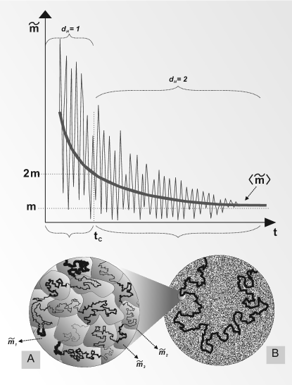
Figure 1: The roughness of the representative trajectories in the relativistic path integral (11) depends on a spatial/temporal scale. On a fine scale (A), where $t\ll t_{C}$ (or $\ell\ll\lambda_{C}$) a particle can be considered as propagating with a sharp Newtonian mass $\tilde{m}$ in a single spatial grain with a Brownian motion controlled by the Hamiltonian ${{\mbox{\boldmath{$p$}}}}^{2}/2\tilde{m}$. On the intermediate scale of order $\lambda_{C}$ the particle propagates with an average velocity equal to the speed of light $c$. On a coarser scale (B) the particle appears to follow a Brownian process with a sharp Lorentz invariant mass $m$, and the particle’s net velocity is then less than $c$ — as it should be for a massive relativistic particle governed by the relativistic Hamiltonian $c({{\mbox{\boldmath{$p$}}}}^{2}+m^{2}c^{2})^{1/2}$.

On more formal level, a stochastic process, representing a relativistic motion on the long-time scale, and described by the Kramers–Moyal equation with the Kramers–Moyal operator $c\sqrt{\hat{{\mbox{\boldmath{$p$}}}}^{2}+m^{2}c^{2}}$, is shown to be equivalent to a doubly stochastic process in which the fast-time dynamics of a free non-relativistic particle (Brownian motion) is coupled with a long-time dynamics describing fluctuations of the particle’s Newtonian mass JK1 .

On more speculative vein, one can fit the above observation into the currently much debated emergent relativity theory, i.e. the approach that tries to view either special or general theory of relativity not as primitive concepts but rather as theories that statistically emerge from a deeper (essentially non-relativistic) level of dynamics bohm:96 ; bohm:93 ; douglas:01 ; jacobson:08 ; Laughlin03 ; Froggatt91 ; Bjorken01 ; Volovik03 .

All these remarks extend directly also to certain interacting systems. For instance, to Dirac’s Hamiltonian JK2

$${H}_{\rm D}^{A,V}=c\gamma_{0}\mbox{\boldmath{$\gamma$}}\cdot({{\mbox{\boldmath{$p$}}}}-e{{\mbox{\boldmath{$A$}}}}/c)+\gamma_{0}(mc^{2}+V)+eA_{0}\,,\;$$ (18)

and to the Feshbach–Villars Hamiltonian JK2

$$\mbox{}{H}_{\rm FV}^{A,V}=(\sigma_{3}+{\rm{i}}\sigma_{2})\frac{1}{2m}({{\mbox{\boldmath{$p$}}}}-e{{\mbox{\boldmath{$A$}}}}/c)^{2}$$

$$\mbox{\hskip 28.45274pt}+\sigma_{3}(mc^{2}+V)+eA_{0}\,.$$ (19)

For example, in the case when $V=0$, $A_{x}=-By$ ($B_{z}\equiv B$), and $A_{y}=A_{z}=0$, then the PI for Dirac’s Hamiltonian yields the “fast scale” Hamiltonian [see JK2 for details]

$$H_{\rm SP}=\frac{1}{2\tilde{m}}\left[\left(p_{x}+\frac{e}{c}By\right)^{\!2}+p_{y}^{2}+p_{z}^{2}\right]-\mu_{\rm B}B\sigma_{3}\,.$$ (20)

This is the Schrödinger–Pauli Hamiltonian with $\mu_{\rm B}=e\hbar/2\tilde{m}$ representing the Bohr magneton. The corresponding grain distribution is again the inverse Gauss distribution. Analogous reasonings can be carried on also for charged spin-$0$ particles, such as, e.g, $\pi^{\pm}$ mesons.

At first sight it may seem rather surprising that a LS process may emerge from a superposition of two non-relativistic stochastic processes. What is perhaps even more surprising is that none of the involved processes has a dynamical symmetry that would correspond to a Lorentz subgroup or to some form of a deformed Lorentz group [see also Calcagni ; Reuter ]. This behavior is, however, less striking when one observes that in many doubly stochastic systems the statistically emergent behavior has a structure vastly different from those of the respective defining processes. Hydrodynamic turbulence provides an example, where the emergent velocity increments and their ensuing Kolmogorov scaling can be understood as originating from two stochastic processes (energy dissipation and chaotic force) operating on two vastly different time scales, despite the fact that none of the processes exhibits any particular scaling structure beckII . Analogous situations are also known from financial markets, e.g., credit risk models or stochastic volatility models.

V Robustness of SR under small variations of mass-smearing distribution

Let us now turn to the question how robust is the emergent special relativity with respect to a slight change in the mass-smearing distribution. In particular, we are asking what is the relation between $\delta\omega$ (or equivalently $\delta f_{1/2}$) and $\delta F$. Such a connection can be easily read off from the relations (4) and (6). Namely,

$$e^{-t[F(s)+\delta F(s)]}\ =\ \int_{0}^{\infty}{\rm{d}}v\ \!e^{-tvs}[\omega(v,t)+\delta\omega(v,t)]\,,$$ (21)

which directly implies

$$-te^{-tF(s)}\delta F(s)\ =\ \int_{0}^{\infty}{\rm{d}}v\ \!e^{-tvs}\delta\omega(v,t)\,.$$ (22)

Because of properties of the Laplace transform, the only solution of Eq. (22) for $\delta F=0$ is $\delta\omega=0$. From this we immediately see that the smearing distribution yielding the left-hand side of (11) is unique insofar as the relativistic Hamiltonian for both positive and negative frequencies has the usual square root form and the dynamics within a “grain” is purely Brownian. So the form of the SR is inexorably connected with the specific structure of the mass-smearing distribution. The aforementioned specificity might be, similarly as in the case of explicit values of the constants of Nature, attributed either to the particular form of initial conditions or to some as yet unknown dynamical mechanism.

The question naturally arising in this connection is how much the SR Hamiltonian $F(H)=\bar{H}({{\mbox{\boldmath{$p$}}}})=c\sqrt{{{\mbox{\boldmath{$p$}}}}^{2}+m^{2}c^{2}}$ changes when small perturbations around the mass-smearing distribution (12) are considered. To answer this question we restrict ourselves to the transformations of the type

$$\hat{t}\ =\ t,\;\;\;\;\;\;\hat{v}\ =\ \hat{v}(v,t)\,.$$ (23)

Since $\omega$ should transform in $v$ as scalar density we have

$$\hat{\omega}(\hat{v},{t})\ =\ \frac{\partial v}{\partial\hat{v}}\ \!\omega(v,t)\,,$$ (24)

or infinitesimally

$$\delta\omega\ =\ \hat{\omega}(v,t)\ -\ \omega(v,t)\ =\ -\frac{\partial}{\partial v}\left(\omega(v,t)\delta v\right)\,.$$ (25)

This also ensures that $\hat{\omega}$ is correctly normalized to $1$. In addition, we require that $\delta\omega(v=0,t)=0$ and $\delta v(v=0,t)=0$, so that $\hat{\omega}(v=0,t)=0$ and the end-point $v=0$ is fixed. Inserting (25) back to Eq. (22) we obtain equivalently

$$\frac{e^{-tF(s)}}{s}\ \!\delta F(s)\ =\ \int_{0}^{\infty}{\rm{d}}v\ \!e^{-tvs}\omega(v,t)\delta v\,.$$ (26)

Because of the condition $\delta v(v=0,t)=0$ we might assume that $\delta v$ can be represented by the series

$$\delta v(v,t)\ =\ v^{\alpha}\sum_{n=0}^{\infty}\epsilon_{n}(t)\ \!v^{n}\,,$$ (27)

where $\alpha\leq 1$ is a positive constant and $\epsilon_{n}(t)\ll 1$ (in order to facilitate small variations in $v$). Through Eq. (25) this also implies that

$$\delta\omega(v,t)\ = -\ \!\omega(v,t)v^{\alpha}\left[\sum_{n=0}^{\infty}v^{n}\left(\frac{t}{4v^{2}}-\frac{3}{2v}\right)\epsilon_{n}(t)\right.$$ (28)

$$+\ \left.\sum_{n=0}^{\infty}v^{n-1}(n+\alpha)\epsilon_{n}(t)\right],$$

which indeed satisfies the required condition $\delta\omega(v=0,t)=0$.

Note further, that (26) can be with the help of (27) written as

$$\delta F(s)\ = \ \sum_{n=0}^{\infty}\epsilon_{n}(t)\ \!\left(\frac{1}{2\sqrt{s}}\right)^{n+\alpha}\!\!K_{n+\alpha-1/2}(t\sqrt{s})$$ (29)

$$\times \ s\ \!e^{t\sqrt{s}}\sqrt{\frac{2t\sqrt{s}}{\pi}}\,.$$

To reveal more details about the previous expansion, let us look at the large-$s$ asymptotic expansion. From theory of modified Bessel functions of the second kind it is known that

$$K_{\nu}(x)\ =\ \sqrt{\frac{\pi}{2}}\frac{e^{-x}}{\sqrt{x}}\left(1+\frac{4\nu^{2}-1}{8x}+\mathcal{O}(1/x^{2})\right)\,,$$ (30)

at $x\rightarrow\infty$ and hence from (29) the leading order terms are

$$\delta F(s)\!\ = \!\ s\!\ \epsilon_{0}(t)\!\left(\frac{1}{2\sqrt{s}}\right)^{\!\alpha}$$ (31)

$$+ \!\ s\left(\frac{1}{2\sqrt{s}}\right)^{\!\alpha+1}\!\left[\epsilon_{1}(t)+\frac{\epsilon_{0}(t)(\alpha^{2}-\alpha)}{t}\right]$$

$$+ \!\ \mathcal{O}(s^{-\alpha/2})\,.$$

So in order to have the RHS $t$ independent, the leading-order coefficient $\epsilon_{0}(t)$ must be time independent, i.e., $\epsilon_{0}(t)=\epsilon_{0}$ and similarly $\epsilon_{1}(t)=\epsilon_{1}-\epsilon_{0}(\alpha^{2}-\alpha)/t$.

On the other hand, the small-$s$ expansion can obtained by observing that upon setting on the RHS of (26) $s=\varepsilon^{-1}$ and $sv=v^{\prime}$ we have

$$\mbox{RHS(\ref{VII.36a})}\ =\ \varepsilon\int_{0}^{\infty}{\rm{d}}v^{\prime}\ \!e^{-tv^{\prime}}\omega(\varepsilon v^{\prime},t)\delta v(\varepsilon v^{\prime},t)\,.$$ (32)

If we now use (27) and expand $\omega(\varepsilon v^{\prime},t)$ for large $\varepsilon$ we can easily find that the leading term in the large-$\varepsilon$ behavior of (32) has the form

$$\mbox{RHS(\ref{VII.36a})}\ \sim\ \epsilon_{0}\ \!t^{1-\alpha}\varepsilon^{\alpha-1/2}\frac{\Gamma\left(\alpha-\mbox{$\frac{1}{2}$}\right)}{2\sqrt{\pi}}\,.$$ (33)

By substituting back $\varepsilon=s^{-1}$ we get

$$\delta F(s)\ \sim\ \epsilon_{0}\ \!t^{1-\alpha}\left(\frac{1}{s}\right)^{\!\alpha-3/2}\frac{\Gamma\left(\alpha-\mbox{$\frac{1}{2}$}\right)}{2\sqrt{\pi}}\,.$$ (34)

The RHS is $t$ independent only if $\alpha=1$. This also implies that the coefficient $\epsilon_{1}(t)$ is time independent, i.e., $\epsilon_{1}(t)=\epsilon_{1}$ (cf. Eq. (31)).

With this preparatory analysis we can now substantially simplify (29). In particular, we can write

$$\mbox{}\delta F(s)\ = \ \epsilon_{0}\frac{\sqrt{s}}{2}$$ (35)

$$+ \ \frac{\epsilon_{1}}{4}\left(1+\frac{1}{\sqrt{s}t}\right)$$

$$+ \ \frac{\epsilon_{2}(t)}{8}\left(\frac{1}{\sqrt{s}}+\frac{3}{st}+\frac{3}{s^{3/2}t^{2}}\right)$$

$$+ \ \epsilon_{3}(t)\left(\frac{1}{s}+\frac{12}{s^{3/2}t}+\frac{60}{s^{2}t^{2}}+\frac{120}{s^{5/2}t^{3}}\right)$$

$$\vdots$$

$$= \ \epsilon_{0}\frac{\sqrt{s}}{2}+\frac{\epsilon_{1}}{4}+\frac{1}{\sqrt{s}}\left(\frac{\epsilon_{1}}{4t}+\frac{\epsilon_{2}(t)}{8}\right)+\ldots\,.$$

So perturbatively (i.e., order by order in the expansions of $\delta v$ and $\delta F$) the LHS can equal to the RHS only when $\epsilon_{0}$ is non-zero and all other $\epsilon_{i}$ are zero. When we wish to include also other $\epsilon_{i}$’s apart from $\epsilon_{0}$ then we must include all of them in order to allow for mutual compensations of their $t$ dependencies. So for instance, we should chose $\epsilon_{2}(t)=\epsilon_{2}-2\epsilon_{1}/t$ in order to get rid of a time dependence in the term $1/\sqrt{s}$. The time dependence in the term with $1/s$ will be canceled by $\epsilon_{3}(t)$, while the time dependence in $1/s^{3/2}$ can be canceled through $\epsilon_{3}(t)$ and $\epsilon_{4}(t)$. In this way one may proceed at infinitum.

To gain insight into implications of the series expansion (35), one may assume (e.g., on convergence ground) that the surviving constant coefficients $\epsilon_{i}$ are decreasing functions of their order “$i$”. One may then hope that a truncation at a suitable higher order term might give analytically manageable and fairly precise form of $\delta F(s)$. In view of Section VII, a particularly pertinent truncation is a truncation that terminates after the $\epsilon_{1}$ term. In this way we include a first non-trivial contribution beyond $\epsilon_{0}$. Note also, that such a truncation must include a part from the $\epsilon_{2}(t)$ term in order to cancel the unwanted $t$ dependence. The resulting expansion reads

$$\delta F(s) = \ \epsilon_{0}\frac{\sqrt{s}}{2}+\frac{\epsilon_{1}}{4}+\frac{1}{\sqrt{s}}\frac{\epsilon_{2}}{8}\,.$$ (36)

To a linear order in $\epsilon_{i}$’s we can write this equivalently as

$$\bar{F}(s)\ = \ F(s)+\delta F(s)$$ (37)

$$\approx \ \frac{\epsilon_{1}}{4}+\left(1+\frac{\epsilon_{0}}{2}\right)\sqrt{s+\frac{\epsilon_{2}}{4}}\,.$$

Here the use was made of the fact that $F(s)=\sqrt{s}$. In order to ensure that $F(0)=0$ we should chose $\epsilon_{1}$ so that

$$\epsilon_{1}\ =\ -2\left(1+\frac{\epsilon_{0}}{2}\right){\sqrt{\epsilon_{2}}}\,.$$ (38)

Let us now turn our attention to the analysis of the result (37). We begin with the observation that the inverse Laplace transform (see Eqs. (4) and (6)) gives us $\hat{\omega}(v,t)$ in the explicit form

$$\mbox{}\hat{\omega}(v,t)\ =\ {\omega}(v,t)+\delta\omega$$

$$\mbox{}=\ \frac{\exp\left\{-\frac{t}{4v}\left[(1+\epsilon_{0}/2)-v\sqrt{\epsilon_{2}}\,\right]^{2}\right\}(1+\epsilon_{0}/2)}{2\sqrt{\pi}\sqrt{v^{3}/t}}\,.$$ (39)

In terms of the mass-smearing distribution this corresponds to the PDF

$$f_{\frac{1}{2}}\!\left(\tilde{m},tc^{2}(1+\epsilon_{0}/2)^{2},tm^{2}c^{2}+\frac{t\epsilon_{2}}{4c^{2}}\right)\,,$$ (40)

and to the associated emergent Hamiltonian

$$\bar{H}\ =\ \frac{\epsilon_{1}}{4}+\left(1+\frac{\epsilon_{0}}{2}\right)\sqrt{{{{\mbox{\boldmath{$p$}}}}^{2}c^{2}+m^{2}c^{4}+\frac{\epsilon_{2}}{4}}}\;.$$ (41)

The ensuing superstatistics PI identity then reads

$$\mbox{}\int_{\footnotesize{{\mbox{\boldmath{$x$}}}}(0)\ \!=\ \!\footnotesize{{\mbox{\boldmath{$x$}}}}^{\prime}}^{\footnotesize{{\mbox{\boldmath{$x$}}}}(t)\ \!=\ \!\footnotesize{{\mbox{\boldmath{$x$}}}}}\ \!{\mathcal{D}}{{\mbox{\boldmath{$x$}}}}\frac{\mathcal{D}{{\mbox{\boldmath{$p$}}}}}{(2\pi)^{D}}\ \!\exp\left\{\int_{0}^{t}\!\!{\rm{d}}\tau\ \!\left[{\rm{i}}{{\mbox{\boldmath{$p$}}}}\cdot\dot{{\mbox{\boldmath{$x$}}}}\ -\ \frac{\epsilon_{1}}{4}-\left(1+\frac{\epsilon_{0}}{2}\right)\sqrt{{{{\mbox{\boldmath{$p$}}}}^{2}c^{2}+m^{2}c^{4}+\frac{\epsilon_{2}}{4}}}\ \,\right]\right\}$$

$$\mbox{}=\ \int_{0}^{\infty}\!\!{\rm{d}}\tilde{m}\ \!f_{\frac{1}{2}}\!\left(\tilde{m},tc^{2}(1+\epsilon_{0}/2)^{2},tm^{2}c^{2}+\frac{t\epsilon_{2}}{4c^{2}}\right)\int_{\footnotesize{{\mbox{\boldmath{$x$}}}}(0)\ \!=\ \!\footnotesize{{\mbox{\boldmath{$x$}}}}^{\prime}}^{\footnotesize{{\mbox{\boldmath{$x$}}}}(t)\ \!=\ \!\footnotesize{{\mbox{\boldmath{$x$}}}}}\ \!{\mathcal{D}}{{\mbox{\boldmath{$x$}}}}\ \!\frac{\mathcal{D}{{\mbox{\boldmath{$p$}}}}}{(2\pi)^{D}}\ \!\exp\left\{\int_{0}^{t}\!\!{\rm{d}}\tau\ \!\left[{\rm{i}}{{\mbox{\boldmath{$p$}}}}\cdot\dot{{\mbox{\boldmath{$x$}}}}-\frac{{{\mbox{\boldmath{$p$}}}}^{2}}{2\tilde{m}}-E_{0}\right]\right\}.$$ (42)

Here

$${E}_{0}\ =\ \left(1+\frac{\epsilon_{0}}{2}\right)\left(\sqrt{{m^{2}c^{4}+\frac{\epsilon_{2}}{4}}}-\frac{\sqrt{\epsilon_{2}}}{2}\,\right),$$ (43)

is the particle’s rest energy implied by $\bar{H}$.

In passing we may note that perturbatively we cannot go beyond a simple re-scaling of the emergent Hamiltonian because in such a case only $\epsilon_{0}$ coefficient is non-trivial. In this latter situation the mass-smearing distribution corresponds to the PDF

$$f_{\frac{1}{2}}(\tilde{m},tc^{2}(1+\epsilon_{0}/2)^{2},tm^{2}c^{2})\,,$$ (44)

and the emergent Hamiltonian has then the form

$$\bar{H}\ =\ \left(1+{\epsilon_{0}}/{2}\right)\sqrt{{{{\mbox{\boldmath{$p$}}}}^{2}c^{2}+m^{2}c^{4}}}\,.$$ (45)

For the future reference this can be cast in the form

$$\bar{H}\ =\ \sqrt{{{{\mbox{\boldmath{$p$}}}}^{2}\bar{c}^{2}+\bar{m}^{2}\bar{c}^{4}}}\,,$$ (46)

with $\bar{c}^{2}=c^{2}(1+\epsilon_{0}/2)^{2}$ and $\bar{m}^{2}=m^{2}/(1+\epsilon_{0}/2)^{2}$.

As a final remark we mention that the key PI identity (42) alongside with the ensuing emergent Hamiltonians (41) and (45) (or (46)) can be nicely fitted into the framework of doubly special relativity. We will return in more detail to this issue in Section VII.

VI The rôle of gauge fixing in emergent Special Relativity

As we have mentioned in Section IV [cf. also Appendices A and B] the superstatistics PI identity (11) implicitly corresponds to a special choice of a gauge, namely to the so called Polyakov or the proper-time gauge. A legitimate question to ask is: what would happen if a different gauge choice is made? After all, a different gauge fixing condition can change the physically preferred foliation of spacetime that is central in our “polycrystalline” picture. But one could equally well turn this question around and ask whether our granular spacetime with its preferred foliation could not be the fundamental (or primitive) concept and the reparametrization invariance only a spurious symmetry related to an inherent redundancy in our description. We shall see in a moment that one may indeed introduce a new redundant variable into the PI on the RHS of (11), in such a way that the new action will have the reparametrization symmetry, but will be still dynamically equivalent to the original action. By not knowing the source, one may then view this artificial gauge invariance as being fundamental or even defining property of the relativistic theory. One might, however, equally well, proclaim the “polycrystalline” picture as being a basic (or primitive) edifice of SR and view the reparametrization symmetry as a mere artefact of an artificial redundancy that is allowed in our description. It is this second view that we favor in this paper.

The trick which will help us to introduce a reparametrization symmetry into the superstatistics PI (11) is akin to the Stückelberg mechanism, whereby one adds a fictitious field to a given system in order to reveal some hidden properties it might possess stuck:38aa ; Goto:67a ; Slavnov:72a . For instance, in quantum electrodynamics one can install gauge symmetry artificially with additional scalar fields, in order to pass from Proca’s ill defined massive Abelian gauge-field theory to renormalizable and gauge invariant massive electromagnetism. Similar field-enlarging transformations are also found useful in non-Abelian Yang–Mills theories Ruegg:04a or in Gravity Hinterbichler:11a .

To proceed, let us introduce a new scalar $\eta$ by making the replacement

$${{\mbox{\boldmath{$x$}}}}\ \mapsto\ {{\mbox{\boldmath{$x$}}}}+\eta{{\mbox{\boldmath{$p$}}}}\,,$$ (47)

which, according to the Süteckelberg prescription, should follow the pattern of the gauge symmetry we want to introduce. In addition, in order to keep the boundary conditions for $x$ we must require $\eta(0)=\eta(t)$. Substituting (47) into the “non-relativistic Lagrangian” in (11) gives

$$L\ = \ {\rm{i}}{{\mbox{\boldmath{$p$}}}}\cdot\dot{{\mbox{\boldmath{$x$}}}}\ -\ \frac{1}{2}\left(\frac{1}{\tilde{m}}-{\rm{i}}\dot{\eta}\right)({{\mbox{\boldmath{$p$}}}}^{2}+m^{2}c^{2})$$ (48)

$$+\ \frac{(\tilde{m}-m)^{2}c^{2}}{2\tilde{m}}\ -\ \frac{\tilde{m}c^{2}}{2}\,.$$

Here we have neglected total derivative terms. Note that the last two terms can be assimilated into a smearing distribution provided we make the redefinition

$$f_{\frac{1}{2}}\!\left(\tilde{m},tc^{2},tc^{2}m^{2}\right)\mapsto f_{\frac{1}{2}}\!\left(\tilde{m},tc^{2},0\right)\,.$$ (49)

Let us further observe that,

$$\delta L = \frac{\delta L}{\delta x^{i}(\tau)}\ \!\delta x^{i}(\tau)+\frac{\delta L}{\delta\eta(\tau)}\ \!\delta\eta(\tau)+\frac{\delta L}{\delta p_{i}(\tau)}\ \!\delta p_{i}(\tau)$$ (50)

$$= \int{\rm{d}}\tau^{\prime}\!\frac{\delta L}{\delta x^{\prime k}(\tau^{\prime})}\left(\!\frac{\delta x^{\prime k}(\tau^{\prime})}{\delta x^{i}(\tau)}\ \!\delta x^{i}(\tau)+\frac{\delta x^{\prime k}(\tau^{\prime})}{\delta\eta(\tau)}\ \!\delta\eta(\tau)\!\right)$$

$$+\ \frac{\delta L}{\delta p_{i}(\tau)}\ \!\delta p_{i}(\tau)\,,$$

and hence the Lagrangian (48) is invariant with respect to the gauge transformation

$$\delta{{\mbox{\boldmath{$x$}}}}(\tau)\ = \ \Lambda(\tau){{\mbox{\boldmath{$p$}}}}(\tau)\,,$$

$$\delta\eta(\tau)\ = \ -\Lambda(\tau)\,,$$

$$\delta{{\mbox{\boldmath{$p$}}}}(\tau)\ = \ {{\mbox{\boldmath{$0$}}}}\,,$$ (51)

where $\Lambda(\tau)$ is an arbitrary function satisfying $\Lambda(0)=\Lambda(t)=0$.

At this stage we observe that modulo a multiplicative constant the RHS of the superstatistics identity (11) can be written as

$$\mbox{(\ref{22a})}\ \!\cong\ \!\int_{\eta(0)=0}^{\eta(t)=0}\mathcal{D}\eta\int_{0}^{\infty}\!\!{\rm{d}}\tilde{m}\ \!f_{\frac{1}{2}}\!\left(\tilde{m},tc^{2},0\right)\int_{\footnotesize{{\mbox{\boldmath{$x$}}}}(0)\ \!=\ \!\footnotesize{{\mbox{\boldmath{$x$}}}}^{\prime}}^{\footnotesize{{\mbox{\boldmath{$x$}}}}(t)\ \!=\ \!\footnotesize{{\mbox{\boldmath{$x$}}}}}\!\!\!\mathcal{D}{{\mbox{\boldmath{$x$}}}}\frac{\mathcal{D}{{\mbox{\boldmath{$p$}}}}}{(2\pi)^{D}}\ \!\exp\left\{\int_{0}^{t}\!\!{\rm{d}}\tau\ \!\!\!\left[{\rm{i}}{{\mbox{\boldmath{$p$}}}}\cdot\dot{{\mbox{\boldmath{$x$}}}}-\frac{1}{2}\left(\frac{1}{{\tilde{m}}}-{\rm{i}}\dot{\eta}\right)({{\mbox{\boldmath{$p$}}}}^{2}+m^{2}c^{2})\right]\right\}\!.$$ (52)

Here we have used the path-integral analogue of the integral identity

$$\int\!{\rm{d}}\eta{\rm{d}}x{\rm{d}}p\ \!f(x+\eta p,p)\ =\ \mathcal{N}\int\!{\rm{d}}x{\rm{d}}p\ \!f(x,p)\,,$$ (53)

with the constant $\mathcal{N}\equiv\int\!{\rm{d}}\eta$.

Let us now define

$$e(\tau)\ =\ \frac{1}{\tilde{m}}\ -\ {\rm{i}}\dot{\eta}(\tau)\,.$$ (54)

This trades the the gauge transformation $\delta\eta(\tau)$ for $\delta e(\tau)=i\dot{\Lambda}(\tau)$. Note further that $e(t)$ fulfils the constraint

$$\int_{0}^{t}{\rm{d}}\tau\ \!e(\tau)\ =\ \frac{t}{\tilde{m}}\,,$$ (55)

which should be included into a function measure for $e(\tau)$ variables in the form of a delta function. The equation (52) can be then equivalently written as

$$\int\mathcal{D}e\int_{0}^{\infty}\!\!{\rm{d}}\tilde{m}\ \delta\left(\int_{0}^{t}{\rm{d}}\tau\ \!e(\tau)-\frac{t}{\tilde{m}}\right)\!f_{\frac{1}{2}}\!\left(\tilde{m},tc^{2},0\right)\int_{\footnotesize{{\mbox{\boldmath{$x$}}}}(0)\ \!=\ \!\footnotesize{{\mbox{\boldmath{$x$}}}}^{\prime}}^{\footnotesize{{\mbox{\boldmath{$x$}}}}(t)\ \!=\ \!\footnotesize{{\mbox{\boldmath{$x$}}}}}\!\mathcal{D}{{\mbox{\boldmath{$x$}}}}\frac{\mathcal{D}{{\mbox{\boldmath{$p$}}}}}{(2\pi)^{D}}\ \!\exp\left\{\int_{0}^{t}\!\!{\rm{d}}\tau\ \!\!\!\left[{\rm{i}}{{\mbox{\boldmath{$p$}}}}\cdot\dot{{\mbox{\boldmath{$x$}}}}-\frac{e}{2}({{\mbox{\boldmath{$p$}}}}^{2}+m^{2}c^{2})\right]\right\}$$

$$=\ \int\mathcal{D}e\ \!\sqrt{\frac{c^{2}t^{2}}{2\pi L^{3}}}\ \!\exp\left(-\frac{t^{2}c^{2}}{2L}\right)\int_{\footnotesize{{\mbox{\boldmath{$x$}}}}(0)\ \!=\ \!\footnotesize{{\mbox{\boldmath{$x$}}}}^{\prime}}^{\footnotesize{{\mbox{\boldmath{$x$}}}}(t)\ \!=\ \!\footnotesize{{\mbox{\boldmath{$x$}}}}}\!\mathcal{D}{{\mbox{\boldmath{$x$}}}}\frac{\mathcal{D}{{\mbox{\boldmath{$p$}}}}}{(2\pi)^{D}}\ \!\exp\left\{\int_{0}^{t}\!\!{\rm{d}}\tau\ \!\!\!\left[{\rm{i}}{{\mbox{\boldmath{$p$}}}}\cdot\dot{{\mbox{\boldmath{$x$}}}}-\frac{e}{2}({{\mbox{\boldmath{$p$}}}}^{2}+m^{2}c^{2})\right]\right\}\!.$$ (56)

Here In particular, the total length of particle’s trajectory is

$$L\ \equiv\ \int_{0}^{t}{\rm{d}}\tau e(\tau)\,.$$ (57)

In connection with (56) we should mention two important points. First, the gauge invariance of the action can be used to reparametrize the time. Indeed, let $\tau\mapsto\tau+\xi(\tau)\equiv\lambda(\tau)$ such that $\xi(0)=\xi(t)=0$. In this case the “action” takes the form

$$\int_{\lambda_{1}}^{\lambda_{2}}{\rm{d}}\lambda\left({\rm{i}}{{\mbox{\boldmath{$p$}}}}\cdot\frac{{\rm{d}}{{\mbox{\boldmath{$x$}}}}}{{\rm{d}}\lambda}-\frac{\tilde{e}}{2}\ \!({{\mbox{\boldmath{$p$}}}}^{2}+m^{2}c^{2})\right)\!,$$ (58)

where

$$\tilde{e}(\lambda)\ =\ e(\tau)\frac{{\rm{d}}\tau}{{\rm{d}}\lambda},$$ (59)

that is, it transforms as the einbein (i.e., a square root of the intrinsic metric along the worldline). In particular, the infinitesimal form of the previous transformation reads

$$\delta e\ =\ -\frac{{\rm{d}}(e\xi)}{{\rm{d}}\tau}\,.$$ (60)

This change can be however assimilated into to gauge transformations of $x$ and $p$ that have the form (cf. (51) and (54))

$$\delta{{\mbox{\boldmath{$x$}}}}\ = \ {\rm{i}}(e\xi){{\mbox{\boldmath{$p$}}}}\,,$$

$$\delta{{\mbox{\boldmath{$p$}}}}\ = \ {{\mbox{\boldmath{$0$}}}}\,.$$ (61)

So Eq.(56) can be equivalently written as

$$\int\mathcal{D}e\ \!\sqrt{\frac{c^{2}t^{2}}{2\pi L^{3}}}\ \!\exp\left(-\frac{t^{2}c^{2}}{2L}\right)\int_{\footnotesize{{\mbox{\boldmath{$x$}}}}(\lambda_{1})\ \!=\ \!\footnotesize{{\mbox{\boldmath{$x$}}}}^{\prime}}^{\footnotesize{{\mbox{\boldmath{$x$}}}}(\lambda_{2})\ \!=\ \!\footnotesize{{\mbox{\boldmath{$x$}}}}}\!\mathcal{D}{{\mbox{\boldmath{$x$}}}}\frac{\mathcal{D}{{\mbox{\boldmath{$p$}}}}}{(2\pi)^{D}}\ \!\exp\left\{\int_{\lambda_{1}}^{\lambda_{2}}\!\!{\rm{d}}\lambda\ \!\left[{\rm{i}}{{\mbox{\boldmath{$p$}}}}\cdot\dot{{\mbox{\boldmath{$x$}}}}-\frac{e}{2}({{\mbox{\boldmath{$p$}}}}^{2}+m^{2}c^{2})\right]\right\}$$

$$=\ -\frac{~{}\partial}{c\ \!\partial t}\int\mathcal{D}e\int_{\footnotesize{x^{\mu}}(\lambda_{1})\ \!=\ \!\footnotesize{x^{\mu}}^{\prime}}^{\footnotesize{x^{\mu}}(\lambda_{2})\ \!=\ \!\footnotesize{x^{\mu}}}\!\mathcal{D}{x^{\mu}}\frac{\mathcal{D}{p_{\mu}}}{(2\pi)^{D+1}}\ \!\exp\left\{\int_{\lambda_{1}}^{\lambda_{2}}\!\!{\rm{d}}\lambda\ \!\left[{\rm{i}}{p}_{\mu}\dot{x}^{\mu}-\frac{e}{2}(p^{2}+m^{2}c^{2})\right]\right\}\!.$$ (62)

In the second line we have utilized an auxiliary Gaussian path integral for $x_{0}$ in the form JK2 ; PI

$$\frac{\partial}{\partial t}\int_{\footnotesize{x_{0}(\lambda_{1})}\ \!=\ \!\footnotesize{0}}^{\footnotesize{x_{0}(\lambda_{2})}\ \!=\ \!\footnotesize{ct}}\!\!\!\mathcal{D}{x_{0}}\frac{\mathcal{D}p_{0}}{(2\pi)}\ \!\exp\left\{\int_{\lambda_{1}}^{\lambda_{2}}\!\!{\rm{d}}\lambda\ \!\left[{\rm{i}}{p}_{0}\ \!\dot{x}_{0}-\frac{e}{2}\ \!p_{0}^{2}\right]\right\}$$

$$=\ -c^{2}t\sqrt{\frac{1}{2\pi L^{3}}}\ \!\exp\left(-\frac{c^{2}t}{2L}\right)\!.$$ (63)

The path integral after the time derivative in (62) is already formulated in a covariant way, as it should be according to Appendix A. At the same time it is well known that this covariant path integral is not completely right (see, e.g., Refs. PI ; polyakov:87 ). In fact, it contains an enormous overcounting, because configurations $(e,x^{\mu},p_{\mu})$ and $(e^{\prime},x^{\prime\mu},p^{\prime}_{\mu})$, that are related to one another by the gauge transformation (51), represent the same physical configuration. One should use any of the standard techniques of constrained quantization, such as, e.g., Faddeev–Popov procedure, to remove this redundancy by imposing appropriately a gauge-fixing condition. For instance, by utilizing the Polyakov (or proper-time) gauge

$$\dot{e}\ =\ 0\,,$$ (64)

the Faddeev–Popov procedure allows to recast (62) into the form

$$\mbox{(\ref{IV63a})}\ =\ -\frac{~{}\partial}{\partial x_{0}}\int_{0}^{\infty}{\rm{d}}L\ \!\int_{\footnotesize{x^{\mu}}(\lambda_{1})\ \!=\ \!\footnotesize{x^{\mu}}^{\prime}}^{\footnotesize{x^{\mu}}(\lambda_{2})\ \!=\ \!\footnotesize{x^{\mu}}}\!\mathcal{D}{x^{\mu}}\frac{\mathcal{D}{p_{\mu}}}{(2\pi)^{D+1}}\ \!\exp\left\{\int_{0}^{L}\!\!{\rm{d}}\lambda\ \!\left[{\rm{i}}{p}_{\mu}\dot{x}^{\mu}-\frac{e}{2}(p^{2}+m^{2}c^{2})\right]\right\}\!.$$ (65)

The expression after $\partial_{x_{0}}$ is nothing but the well known Feynman–Fock world-line representation of the KG propagator JK2 ; FH ; PI ; polyakov:87 . In addition, in this particular gauge the PI form (65) explicitly coincides with the superstatistics PI (11) as the reader can easily observe by performing the $x_{0}$ and $p_{0}$ functional integrations.

From the previous considerations we see that the Stückelberg trick is a terrific illustration of the fact that the reparametrization invariance of a quantum relativistic particle can be regarded as a mathematical sham. It represents nothing more than a redundancy of description. In practice one could take any theory and form from it a gauge theory by introducing redundant variables along the presented lines. Conversely, given any gauge theory, one can always eliminate the gauge symmetry by eliminating the redundant degrees of freedom. The drawback is that removing the redundancy is not always a smart thing to do. In fact, it is often said that gauge symmetry is fundamental as, for instance, in electromagnetism. A more accurate statement is, however, that the gauge symmetry in electromagnetism is necessary only if one demands the convenience of linearly realized LS and locality. Fixing a gauge will not change the physics, but the price paid is that the LS and locality are not necessarily manifest. This is precisely what has happened in the case of the FV equation. There, the particular choice of a gauge in which the equation is formulated leads to a non-linear realization of the LS (see Appendix A in Ref. JK2 where the associated non-linear realization is discussed).

In conclusion, the previous construction shows clearly that the polycrystalline spacetime picture may be legitimately considered as the primitive conceptual framework for a relativistic quantum particle. On the other hand, the assumptions like the reparametrization invariance, which lie at the bedrock of relativistic quantum mechanics, cannot be held immune to scrutiny. In fact, we have seen that the reparametrization symmetry, can be perceived as a mere artefact of an underlying (spurious) redundancy of the description. In other words, the reparametrization symmetry can be seen as being derived, rather than primitive edifice of relativistic quantum mechanics.

In what follows we propose an unifying approach for Special and Doubly Special Relativity, based on the existing laws of quantum mechanics as formulated through superstatistics PI’s.

VII Emergent Doubly Special Relativity

Our analysis from Section V reveals what kind of dynamical systems should be expected when the underlying mass-smearing (or equivalently grain-size) distribution is slightly deformed. Under a fairly general set of assumptions, we have arrived there at the emergent Hamiltonian (41) and its “contracted” version (45). In this section we are going to see in more detail, that the dynamics associated with the aforementioned Hamiltonians can be identified with the so-called Doubly (or Deformed) Special-Relativistic dynamics.

In a nutshell, DSR is a theory which coherently tries to implement a second invariant, besides the speed of light, into the transformations among inertial reference frames. This new invariant comes directly from the research in quantum gravity, and it is usually assumed to be an observer-independent length-scale — the Planck length $\ell_{p}$, or its inverse, i.e., the Planck energy $E_{p}=c\ell_{p}^{-1}$. Thus, it is not so surprising that the relations mainly studied are those between DSR and various quantum gravity models Smolin ; GirOr1 ; Rovelli . In a particularly suggestive approach GirOr2 , DSR has been presented as the low energy limit of Quantum Gravity. Connections between DSR and other theories (non commutative geometry, AdS space-time, etc.) have also been recently investigated GirLiv .

It is by now well acknowledged that the DSR stands among the prominent ideas introduced in physics during the last decade, and also among the most controversial ones. Many foundational issues about this theory are still being debated, in particular for example the multi-particle sector of the theory (the so called Soccer Ball Problem) Kowalski . An important area of investigation has been that of the relations between DSR and other theoretical construction of modern physics.

Clearly, the most important connection is the one between DSR and Special Relativity (SR) itself. However in literature does not exist any conceptually deeper elaboration of this connection, apart form the obvious statement that for energy scales much smaller than $E_{p}$, DSR should reduce to conventional SR, with leading corrections of first or higher order in the ratio of energy scales to $E_{p}$. In this respect, the findings of the present paper seem to open up new vistas. In fact, when the microstructure of space-time is considered, then Special Relativity or DSR seem to emerge from particular choices of such microstructure itself, and from a non-relativistic Hamilton (i.e., phase-space) mechanics.

To extend our reasonings to DSR, we start by considering the modified invariant, or deformed dispersion relation,

$$\frac{\eta^{ab}p_{a}p_{b}}{(1-\ell_{p}p_{0})^{2}}\ =\ m^{2}c^{2}\,,$$ (66)

proposed by Magueijo and Smolin Mag ; Mag2 . Here $m$ plays the role of the DSR invariant mass. Assuming a metric signature $(+,-,-,-)$, we can solve (66) in respect to $p_{0}$, which essentially coincides with the physical Hamiltonian $\bar{H}=cp_{0}$. The latter is the generator of the temporal translations with respect to the coordinate time $t$. Our starting Hamiltonian is therefore

$$\bar{H}\ =\ c\ \!\frac{{-m^{2}c^{2}\ell\mp\sqrt{{{\mbox{\boldmath{$p$}}}}^{2}(1-m^{2}c^{2}\ell^{2})+m^{2}c^{2}}}}{1-m^{2}c^{2}\ell^{2}}\,,$$ (67)

which we assume as the transformed Hamiltonian $\bar{H}(p,x)=F(H(p,x))$ entering the proper PI representation of $\bar{P}(x_{b},t_{b}|x_{a},t_{a})$, see Eq. (6) and the comments below [see also Ref. JK1 ]. Note that by setting

$$\epsilon_{1}\ = \ 2\left(\sqrt{\frac{1}{1-c^{2}m^{2}\ell^{2}}}\ \!-\ \!1\right),$$

$$\epsilon_{2}\ = \ \frac{4c^{6}m^{4}\ell^{2}}{1-c^{2}m^{2}\ell^{2}}\,,$$ (68)

we can identify the DSR Hamiltonian (67) with the Hamiltonian (41) obtained in Section V. In close analogy with (11), it is now possible to show the superstatistics identity [see Appendix C]

$$\mbox{}\int_{\footnotesize{{\mbox{\boldmath{$x$}}}}(0)\ \!=\ \!\footnotesize{{\mbox{\boldmath{$x$}}}}^{\prime}}^{\footnotesize{{\mbox{\boldmath{$x$}}}}(t)\ \!=\ \!\footnotesize{{\mbox{\boldmath{$x$}}}}}\ \!{\mathcal{D}}{{\mbox{\boldmath{$x$}}}}\frac{\mathcal{D}{{\mbox{\boldmath{$p$}}}}}{(2\pi)^{D}}\ \!\exp\left\{\int_{0}^{t}\!\!{\rm{d}}\tau\ \!\left[{\rm{i}}{{\mbox{\boldmath{$p$}}}}\cdot\dot{{\mbox{\boldmath{$x$}}}}\ +\ c\frac{\left({m^{2}c^{2}\ell-\sqrt{{{\mbox{\boldmath{$p$}}}}^{2}(1-m^{2}c^{2}\ell^{2})+m^{2}c^{2}}}\right)}{(1-m^{2}c^{2}\ell^{2})}\right]\right\}$$

$$\mbox{\hskip 34.1433pt}=\ \int_{0}^{\infty}\!\!{\rm{d}}\tilde{m}\ \!f_{\frac{1}{2}}\!\left(\tilde{m},tc^{2}\lambda,tc^{2}m^{2}\lambda\right)\int_{\footnotesize{{\mbox{\boldmath{$x$}}}}(0)\ \!=\ \!\footnotesize{{\mbox{\boldmath{$x$}}}}^{\prime}}^{\footnotesize{{\mbox{\boldmath{$x$}}}}(t)\ \!=\ \!\footnotesize{{\mbox{\boldmath{$x$}}}}}\ \!{\mathcal{D}}{{\mbox{\boldmath{$x$}}}}\ \!\frac{\mathcal{D}{{\mbox{\boldmath{$p$}}}}}{(2\pi)^{D}}\ \!\exp\left\{\int_{0}^{t}\!\!{\rm{d}}\tau\ \!\left[{\rm{i}}{{\mbox{\boldmath{$p$}}}}\cdot\dot{{\mbox{\boldmath{$x$}}}}-\frac{{{\mbox{\boldmath{$p$}}}}^{2}}{2\tilde{m}}-E_{0}\right]\right\},$$ (69)

where $E_{0}=mc^{2}/(1+mc\ell)$ is the particle’s rest energy [see, e.g., Mag2 ] and $\lambda=1/(1-m^{2}c^{2}\ell^{2})$ is the deformation parameter. From (12), it is easy to see that $\langle\tilde{m}\rangle=m+1/(tc^{2}\lambda)$ and var$(\tilde{m})=m/tc^{2}\lambda+2/t^{2}c^{4}\lambda^{2}$.

From the structure of $\langle\tilde{m}\rangle$ we can obtain further useful insights. Similarly as in the SR framework, the fluctuating Newtonian mass $\tilde{m}$ converges rapidly, at long times $t$, to the SR rest mass $m$. But in this case is the rate of convergence controlled also by the parameter $\lambda$. Reminding that $E_{p}=c/\ell_{p}$, we see that $\lambda=1/(1-E^{2}/E_{p}^{2})$. So, $\langle\tilde{m}\rangle$ can converge rapidly to the Einstein value $m$, even at short times, provided that the particle’s energy $E$ be close to the Planck energy $E_{p}$. The correlation distance is now given by $\sim 1/(mc\lambda)$, and since $\lambda>1$, then $1/(mc\lambda)<1/(mc)$ always.

From the identity (69) we can quickly deduce the CCR via the standard PI analysis. In particular the CCR can be directly related to the degree of roughness (described through Hausdorff dimension $d_{H}$ or Hurst exponent $h$) of typical PI paths Kroger ; FH . For instance, the usual non-relativistic canonical relation $[\hat{{{\mbox{\boldmath{$x$}}}}}_{i},\hat{{{\mbox{\boldmath{$p$}}}}}_{j}]={\rm{i}}\delta_{ij}$ results from the fact that, for a typical path occurring in non-relativistic PI’s, $d_{H}$ and $h$ are $2$ and $1/2$, respectively. In fact, in non-relativistic quantum mechanics all local potentials fall into the same universality class (as for the scaling behavior) as the free system Kroger . The latter might be viewed as a PI justification of the universal form of non-relativistic CCR’s.

It is not hard to show [cf. Appendix D] that the PI identity (69) implies the commutators

$$[\hat{{\mbox{\boldmath{$x$}}}}_{i},\hat{{\mbox{\boldmath{$p$}}}}_{j}]_{\rm DSR1}\ =\ {\rm{i}}\!\left(\delta_{ij}+\frac{\kappa^{2}-m^{2}c^{2}}{\kappa^{2}m^{2}c^{2}}\ \!\hat{{\mbox{\boldmath{$p$}}}}_{i}\hat{{\mbox{\boldmath{$p$}}}}_{j}\right)\!.$$ (70)

Here $\kappa=1/\ell$. The CCR (70) resembles the Snyder version of the deformed CCR associated to the dispersion relation (66) [cf. Refs. Snyder:47 ; Ghosh:07 ; Ghosh:06 ; Banerjee:06 ]. To be precise, the Snyder fundamental commutation relation [see Ref. Snyder:47 ] in the notation of the present paper (for $\hbar=1$, the Snyder fundamental length $a\equiv\ell=1/\kappa$) would read

$$[\hat{{\mbox{\boldmath{$x$}}}}_{i},\hat{{\mbox{\boldmath{$p$}}}}_{j}]_{\rm Snyder}\ =\ {\rm{i}}\!\left(\delta_{ij}+\frac{\hat{{\mbox{\boldmath{$p$}}}}_{i}\hat{{\mbox{\boldmath{$p$}}}}_{j}}{\kappa^{2}}\ \!\right)\!.$$ (71)

So the prefactor of the deforming term in the Snyder commutator is a constant related to the fundamental length, while in the DSR commutator (70) the prefactor varies with the Einstein mass of the particle considered. The minimal length interval $\ell$ is typically set to be the Planck length $\ell_{p}$, or more generally to be the Compton length $\lambda_{C}$ (which reduces to the Planck length for a Planck mass). For definiteness we will in the following identify $\ell$ with $\ell_{p}$. In this connection, note that when $mc\to\kappa$, i.e., when $m$ coincides with the Planck mass, then the CCR (70) becomes non-relativistic. This can also be directly seen from (69), where for $m\to M_{p}$ the defromation parameter $\lambda\to\infty$, and the smearing distribution $f_{\frac{1}{2}}\!\left(\tilde{m},tc^{2}\lambda,tc^{2}m^{2}\lambda\right)\to\delta(m-\tilde{m})$, which yields the usual PI for a Wiener process.

Should we have used instead of (66) a different DSR dispersion relation, for example

$$\frac{p_{0}^{2}-{\bf p}^{2}}{1-(\ell_{p}p_{0})^{2}}\ =\ m^{2}c^{2}\,,$$ (72)

(which is discussed in Ref. Mag3 ), we would have obtained the DSR Hamiltonian

$$\bar{H}\ =\ \pm\ \!\frac{\sqrt{{{\mbox{\boldmath{$p$}}}}^{2}c^{2}+m^{2}c^{4}}}{\sqrt{1+m^{2}c^{2}\ell^{2}}}\,,$$ (73)

from which follows the superstatistics identity [see again Appendix C]

$$\mbox{}\int_{\footnotesize{{\mbox{\boldmath{$x$}}}}(0)\ \!=\ \!\footnotesize{{\mbox{\boldmath{$x$}}}}^{\prime}}^{\footnotesize{{\mbox{\boldmath{$x$}}}}(t)\ \!=\ \!\footnotesize{{\mbox{\boldmath{$x$}}}}}\ \!{\mathcal{D}}{{\mbox{\boldmath{$x$}}}}\frac{\mathcal{D}{{\mbox{\boldmath{$p$}}}}}{(2\pi)^{D}}\ \!\exp\left\{\int_{0}^{t}\!\!{\rm{d}}\tau\ \!\left[{\rm{i}}{{\mbox{\boldmath{$p$}}}}\cdot\dot{{\mbox{\boldmath{$x$}}}}\ -\ \frac{\sqrt{{{\mbox{\boldmath{$p$}}}}^{2}c^{2}+m^{2}c^{4}}}{\sqrt{1+m^{2}c^{2}\ell^{2}}}\right]\right\}$$

$$\mbox{\hskip 34.1433pt}=\ \int_{0}^{\infty}\!\!{\rm{d}}\tilde{m}\ \!f_{\frac{1}{2}}\!\left(\tilde{m},tc^{2}{\zeta}^{2},tc^{2}m^{2}\right)\int_{\footnotesize{{\mbox{\boldmath{$x$}}}}(0)\ \!=\ \!\footnotesize{{\mbox{\boldmath{$x$}}}}^{\prime}}^{\footnotesize{{\mbox{\boldmath{$x$}}}}(t)\ \!=\ \!\footnotesize{{\mbox{\boldmath{$x$}}}}}\ \!{\mathcal{D}}{{\mbox{\boldmath{$x$}}}}\ \!\frac{\mathcal{D}{{\mbox{\boldmath{$p$}}}}}{(2\pi)^{D}}\ \!\exp\left\{\int_{0}^{t}\!\!{\rm{d}}\tau\ \!\left[{\rm{i}}{{\mbox{\boldmath{$p$}}}}\cdot\dot{{\mbox{\boldmath{$x$}}}}-\frac{{{\mbox{\boldmath{$p$}}}}^{2}}{2\tilde{m}}-\bar{E}_{0}\right]\right\}.$$ (74)

Here $\bar{E}_{0}=mc^{2}/\sqrt{1+m^{2}c^{2}\ell^{2}}$ is the particle’s rest energy and the deformation parameter now reads $\zeta=1/\sqrt{1+m^{2}c^{2}\ell^{2}}$. It is not difficult to compute that $\langle\tilde{m}\rangle=m/{\zeta}+1/(c^{2}t{\zeta}^{2})$ and var$(\tilde{m})={m}/({tc^{2}\zeta^{3}})+{2}/({t^{2}c^{4}\zeta^{4}})$. Let us observe that this double-special relativity model does not have the desired property that its fluctuating mass converges to a Lorentz mass in the large $t$ limit. In addition, because $\zeta\in(0,1)$, the fluctuations at short times cannot be suppressed and one thus cannot hope to have a relativistic system with a sharp Einsteinian mass at the Planck energy. In passing, we may note that the DSR system (73) coincides with system (45)-(46) from Section V provided we make identification

$$\epsilon_{0}\ =\ 2\left(\zeta\ \!-\ \!1\right).$$ (75)

The CCR in this system read [cf. Appendix D]

$$[\hat{{\mbox{\boldmath{$x$}}}}_{j},\hat{{\mbox{\boldmath{$p$}}}}_{i}]_{\rm DSR2}\ = \ {\rm{i}}\!\left(\delta_{ij}+\!\frac{\hat{{\mbox{\boldmath{$p$}}}}_{i}\hat{{\mbox{\boldmath{$p$}}}}_{j}}{m^{2}c^{2}}\right)\!.$$ (76)

As the reader can see, this commutator coincides with the SR one. Some comments on this apparently surprising fact are contained in Appendix D.

At this point, for the sake of completeness, we should also note that commutator (70) does not coincide with the commutator (61) of the Magueijo–Smolin paper Mag2 , although it comes from the same dispersion relation (66), proposed in Mag2 as formula (3). Moreover, both commutators (70) and (76) do not enjoy an important property of the commutator (61) from Ref. Mag2 . In fact, when the energy of the boosted system approaches the Planck energy, the aforementioned commutator, which reads

$$[\hat{{\mbox{\boldmath{$x$}}}}_{j},\hat{{\mbox{\boldmath{$p$}}}}_{i}]_{\rm MS}\ = \ {\rm{i}}\,\delta_{ij}\left(1-\frac{E}{E_{p}}\right)\!,$$ (77)

goes to zero, and so it predicts the appearance of a classical world at the Planck scale. On the contrary, when the energy of the particle under boost approaches the Planck value, commutators (70) and (76) become respectively

$$[\hat{{\mbox{\boldmath{$x$}}}}_{j},\hat{{\mbox{\boldmath{$p$}}}}_{i}]_{\rm{DSR1}}\ =\ {\rm{i}}\,\delta_{ij}\,,$$

$$[\hat{{\mbox{\boldmath{$x$}}}}_{j},\hat{{\mbox{\boldmath{$p$}}}}_{i}]_{\rm{DSR2}}\ =\ {\rm{i}}\left(\delta_{ij}+\frac{\hat{{\mbox{\boldmath{$p$}}}}_{i}\hat{{\mbox{\boldmath{$p$}}}}_{j}}{\kappa^{2}}\right)\,.$$ (78)

The qualitative difference in behavior of both CCR can be traced back to the fact that commutators in (doubly-)special relativity depend on two things; First, the fundamental commutators are essentially the Dirac brackets of the canonical variables. The explicit definition of the Dirac brackets depends on the choice of a gauge (gauge fixing condition), which for relativistic systems corresponds to choice of a specific physical time. So the commutation relations are generally gauge fixing dependent in both SR and DSR systems. Second, the fundamental commutator $[\hat{{\mbox{\boldmath{$x$}}}}_{j},\hat{{\mbox{\boldmath{$p$}}}}_{i}]$ depends (through the Jacobi identities) on the whole symplectic structure of the system (and therefore also on the commutator $[\hat{{\mbox{\boldmath{$x$}}}}_{j},\hat{{\mbox{\boldmath{$x$}}}}_{i}]$, for example). These are not specified by a particular DSR model, but they have to be chosen aside. Of course, one obtains different theories for different choices of $[\hat{{\mbox{\boldmath{$x$}}}}_{j},\hat{{\mbox{\boldmath{$x$}}}}_{i}]$.

In our specific path-integral approach, the gauge which is automatically incorporated in the path integral is the Polyakov gauge. We obtain the same fundamental commutator of Ghosh Ghosh:07 . For Ghosh Ghosh:07 and Mignemi Mignemi the $\hat{{\mbox{\boldmath{$x$}}}}_{j}$’s do not commute, $[\hat{{\mbox{\boldmath{$x$}}}}_{j},\hat{{\mbox{\boldmath{$x$}}}}_{i}]\neq 0$, while on the contrary Magueijo–Smolin in Mag2 require the $\hat{{\mbox{\boldmath{$x$}}}}_{j}$’s to commute (formula (60)).

So, a DSR theory is not only defined by the dispersion relation, but also by the gauge fixing and the choice of the symplectic structure, which is essentially arbitrary. In principle, therefore, only the experiment can effectively discriminate among different models. It should now become clear why our model can produce commutators different from those of Ref. Mag2 , although both models share the same deformed dispersion relation. As a small further note, we may add that from the Magueijo–Smolin paper Mag2 it is not clear if the proposed commutators satisfy the Jacobi identities or not (not enough commutators are, in fact, explicitly specified to enable the reader to verify the Jacobi identity).

We conclude with an important observation. Should we have applied our analysis from Section V to the above DSR systems we would have obtained that a slight perturbation in the mass-smearing distribution would yield again DSR systems. From this standpoint is the DSR (as well as its low-energy limit — SR) a robust concept, i.e. its algebraic structure continues to hold despite (potentially dynamical) alterations in polycrystalline structure conditions.

VIII Concluding remarks

In this paper we have shown that both SR and DSR systems can arise by statistically coarse-graining underlying non-relativistic (Wiener) process, making the latter more fundamental and the former in some sense emergent. The coarse-graining can be viewed as arising from superposition of two stochastic processes. On a short spatial scale (much shorter than particle’s Compton wavelength) the particle moves according to a Brownian, non-relativistic, motion. Its Newtonian mass fluctuates according to an inverse Gaussian distribution.

The time-compounded smearing distribution tends, however, rapidly to the delta-function distribution due to the central limit theorem. This happens at the time scale of the order of Compton time, at which the relative mass fluctuation is of order unity. The Compton length also represents the critical length scale at which the Feynman–Hibbs scaling relation between $\Delta x$ and $\Delta t$ changes its critical exponent (Hurst exponent) from $1$ to $1/2$. The Compton time and ensuing Compton length can be thus viewed as correlation time and correlation length, respectively. The averaged (or coarse-grained) velocity over the correlation time is the light velocity $c$. On a time scale much larger than the Compton time, the particle then behaves as a relativistic particle with a sharp mass equal to Einstein’s (i.e., Lorentz invariant) mass. In this case the particle moves with a net velocity which is less than $c$. Here the reader may notice a close analogy with the Feynman chessboard PI. In contrast to the chessboard PI, our approach is not confined to only $1+1$ dimensional Dirac fermions.

The presented concept of statistical emergence, which is shared both by SR and DSR, can offer a new valid insight into the Planck-scale structure of space-time. The existence of a discrete polycrystalline substrate (or vacuum) might be welcomed in various quantum gravity constructions. In fact, it has been speculated for long time that quantum gravity may lead to a discrete structure of space and time which can cure classical singularities. This idea has been embodied, in particular, in Loop Quantum Cosmology Ashtekar ; Bojowald . A similar proposal was put forward in Ref. Vilenkin in connection with the space-time foam. It should be stressed that many condensed matter systems show that a discrete sub-structure might lead to a genuinely relativistic dynamics at low energies Volovik03 , without any internal inconsistency. A paradigmatic example of this are wide single-layer carbon crystals (graphene), where an effective theory emerges in which conducting electrons behave, at low temperatures, as massless relativistic Dirac fermions with a “light speed” equal to the Fermi velocity of the crystal Novoselov:05 . Essentially the same emergent behavior is known to hold also for silicene, i.e., the monolayer silicon equivalent of graphene Vogt:12a .

In this connection one can also stress that crystal-like substrates — discrete lattices, are routinely used, for instance, in computational quantum field theory KleinertIII ; Creutz:83 ; FIRST where the genuine relativistic field dynamics emerges only in the long-wavelength limit, i.e., at distances much larger than a typical lattice spacing. However, with a few notable exceptions Friedberg:83a ; Friedberg:83b , the lattices is these case mainly serve as numerical regulators of ultraviolet divergences. Indeed, a crucial point of renormalized theories is precisely to extract lattice-independent data from numerical computations.

We close this paper with a number of questions, to be examined in a future work. Foremost: We have stressed that the proposed coarse-graining view directly applies also to simple interacting systems, such as the Dirac’s particle in a constant external electromagnetic potential. One may naturally wonder whether this interpretation can be extended to more general interacting systems. So far, two points hinder this program to be carried further in a full generality: first, the general $x$-dependence of $A_{\mu}$ and $V$ leads to a notorious ordering problem. Second, and most important, the transformation that would bring the Hamiltonian into a form where the positive and negative energy parts are explicitly separated is no longer possible for a general interaction. This last point makes it difficult to carry over straightforwardly our reasonings. On the other hand, if the proposed picture aspires to be more than just an interesting metaphor, one should be able to demonstrate the viability of our scheme also for less trivial interactions. It remains yet to be seen to what extent this can be done.

Another open issue is the rôle of the smearing distribution. In the presented approach, the specific form of the smearing distribution is a mere byproduct of the superstatistics PI paradigm. Our heuristic picture of a polycrystalline medium which we affiliate with the smearing distribution is clearly not the only possibility. Furthermore, a deeper understanding of a dynamical origin of our smearing would be highly desirable. In fact, the exact LS is due to a very special form of the Newtonian-mass distribution. The exact LS of a spacetime has no fundamental significance in our model, but it is only an accidental symmetry of the spatially coarse-grained theory. This “accidentalness” is controlled by a specific form of the grain distribution. We have seen that a small departure from its shape brings a departure from LS and leads naturally to the DSR. In this respect a useful guide to understanding the specificity of grain distributions could be the observation that generalized inverse Gaussian distributions with $p=1/2$ correspond (among others) to first-hitting inverse-time PDF’s Barndorff:78 . This might indicate that our smearings distribute inverse times (i.e., masses) between successive events in a renewal process (such as a passage to a new grain). The latter would, in a sense, support our polycrystalline picture.

Finally, it is also hoped that the essence of our results will continue to hold in curved spacetimes. This could be an important step in addressing the issue of quantum gravity. In this connection we may notice a conceptual similarity with the Hořava–Lifshitz gravity theory Horava , where, as in our case, space and time are not equivalent at the fundamental level, and therefore the theory is intrinsically non-relativistic. The relativistic concept of time together with its Lorentz invariance emerges at distances much larger than Compton wavelength.

Appendix A 

Here we briefly review, without going to much details, some essentials related to PI representation of the Klein–Gordon particle in the Feshbach–Villars representation.

The doubling of the wave function in Eq. (10) implies the simultaneous description of particles and antiparticles Feshbach58 . The Hamiltonian ${H}_{{}_{\rm FV}}({{\mbox{\boldmath{$p$}}}})$ can be diagonalized as

$$\hat{H}_{{}_{\rm FV}}({{\mbox{\boldmath{$p$}}}})\ =\ {U}({{\mbox{\boldmath{$p$}}}})\sigma_{3}{U}({{\mbox{\boldmath{$p$}}}})^{-1}\hat{H}({{\mbox{\boldmath{$p$}}}})\,,$$ (79)

where $U$ is non-unitary hermitian matrix

$${U}({{\mbox{\boldmath{$p$}}}})=\frac{(1+\gamma_{v})+(1-\gamma_{v})\sigma_{1}}{2\sqrt{\gamma_{v}}}\,,$$ (80)

$\hat{H}({{\mbox{\boldmath{$p$}}}})=c\sqrt{\hat{{\mbox{\boldmath{$p$}}}}^{2}+m^{2}c^{2}}$ is the energy operator, and $\gamma_{v}=1/\sqrt{1-v^{2}/c^{2}}$. The Green’s function ${\mathcal{G}}(x,y)$ associated with the FV Schrödinger equation can be written as

$${\mathcal{G}}(x;y)\ =\ \frac{{\rm{i}}}{c^{2}}\int_{\mathbb{R}^{4}}\frac{{\rm{d}}^{D+1}p}{(2\pi)^{D+1}}\ \!\frac{e^{-\footnotesize{{\rm{i}}}p(x-y)}}{p^{2}-m^{2}c^{2}+{\rm{i}}\epsilon}\ \!\left[p_{{}_{0}}c+(\sigma_{3}+{\rm{i}}\sigma_{2})\frac{{{\mbox{\boldmath{$p$}}}}^{2}}{2m}+\sigma_{3}mc^{2}\right]\,.$$

Here the ${\rm{i}}\epsilon$ prescription corresponds to the usual Feynman boundary condition. Note that the imaginary-time Green function $\mathcal{G}({{\mbox{\boldmath{$x$}}}},-it;{{\mbox{\boldmath{$x$}}}}^{\prime},-it^{\prime})\equiv P({{\mbox{\boldmath{$x$}}}},t|{{\mbox{\boldmath{$x$}}}}^{\prime},t^{\prime})$ is a solution of the Fokker–Planck like equation $(\partial_{t}+\hat{H}_{{}_{\rm FV}})P({{\mbox{\boldmath{$x$}}}},t|{{\mbox{\boldmath{$x$}}}},t^{\prime})\ =\ \delta(t-t^{\prime})\delta^{(3)}({{\mbox{\boldmath{$x$}}}}-{{\mbox{\boldmath{$x$}}}}^{\prime})$, where $P({{\mbox{\boldmath{$x$}}}},t|{{\mbox{\boldmath{$x$}}}}^{\prime},t^{\prime})=\langle{{\mbox{\boldmath{$x$}}}}|e^{-(t-t^{\prime})\hat{H}_{{}_{\rm FV}}}|{{\mbox{\boldmath{$x$}}}}^{\prime}\rangle$. Because of (79), the latter can be equivalently written as

$$P({{\mbox{\boldmath{$x$}}}},t|{{\mbox{\boldmath{$x$}}}}^{\prime},t^{\prime})=\int_{\mathbb{R}^{D}}{\rm{d}}{{\mbox{\boldmath{$x$}}}}^{\prime\prime}\int_{\mathbb{R}^{D}}\frac{{\rm{d}}{{\mbox{\boldmath{$p$}}}}}{(2\pi)^{D}}\ \!\ \!{e^{{\rm{i}}\small{{{\mbox{\boldmath{$p$}}}}\ \!\cdot({{\mbox{\boldmath{$x$}}}}-{{\mbox{\boldmath{$x$}}}}^{\prime\prime})}}}\ \!U({{\mbox{\boldmath{$p$}}}})\langle{{\mbox{\boldmath{$x$}}}}^{\prime\prime}|e^{-(t-t^{\prime})\sigma_{3}\hat{H}({\footnotesize{{\mbox{\boldmath{$p$}}}}})}|{{\mbox{\boldmath{$x$}}}}^{\prime}\rangle U({{\mbox{\boldmath{$p$}}}})^{-1}\,.$$

At this point a warning should be made, that we cannot write naively the PI representation of $\langle{{\mbox{\boldmath{$x$}}}}|e^{-(t-t^{\prime})\sigma_{3}\hat{\!H}({\footnotesize{{\mbox{\boldmath{$p$}}}}})}|{{\mbox{\boldmath{$x$}}}}^{\prime}\rangle$ by considering $\sigma_{3}\hat{\!H}({\footnotesize{{\mbox{\boldmath{$p$}}}}})$ as a formal Hamiltonian. This is because the PI with the ensuing action $\int_{t^{\prime}}^{t}{\rm{d}}\tau\left[{\rm{i}}\small{{\mbox{\boldmath{$p$}}}}\cdot\dot{\small{{\mbox{\boldmath{$x$}}}}}-c\sigma_{3}\sqrt{\small{{\mbox{\boldmath{$p$}}}}^{2}+m^{2}c^{2}}\right]$ would diverge. The pathology involved can be evaded by forming superpositions of integrals which differ for upper and lower components of $\exp(-t\sigma_{3}\hat{H}{({\mbox{\boldmath{$p$}}}}))$ according to Feynman–Stuckelberg prescription, i.e., we consider positive frequencies as propagating forward in time and negative frequencies backward in time. This yields the well behaved PI [cf. Ref. JK2 ]

$$\langle{{\mbox{\boldmath{$x$}}}}|e^{-t\sigma_{3}\hat{H}({\footnotesize{{\mbox{\boldmath{$p$}}}}})}|{{\mbox{\boldmath{$x$}}}}^{\prime}\rangle\ =\ \int_{0}^{\infty}{\rm{d}}v\ \!\omega(v,t)\int_{\footnotesize{{\mbox{\boldmath{$x$}}}}(0)\ \!=\ \!\footnotesize{{\mbox{\boldmath{$x$}}}}^{\prime}}^{\footnotesize{{\mbox{\boldmath{$x$}}}}(t)\ \!=\ \!\footnotesize{{\mbox{\boldmath{$x$}}}}}\ \!\mathcal{D}{{{\mbox{\boldmath{$x$}}}}}\frac{\mathcal{D}{{{\mbox{\boldmath{$p$}}}}}}{(2\pi)^{D}}\ \!\exp\left\{\int_{0}^{t}{\rm{d}}\tau\left[{\rm{i}}{{\mbox{\boldmath{$p$}}}}\cdot\dot{{\mbox{\boldmath{$x$}}}}-v({{{\mbox{\boldmath{$p$}}}}^{2}c^{2}+m^{2}c^{4})}\right]\right\}\,.$$

The weight function is now a matrix valued Weibull distribution

$$\omega(v,t)\ =\ \frac{1}{2\sqrt{\pi}\sqrt{{v^{3}}/{|t|}}}\left(\begin{array}[]{cc}\theta(t)\ \!e^{-t/4v}&0\\ 0&\theta(-t)\ \!e^{t/4v}\\ \end{array}\right)\!.$$ (86)

At the same time we can write

$$\mbox{}\langle{{\mbox{\boldmath{$x$}}}}|{\rm{e}}^{-t\sigma_{3}\hat{\!H}({\footnotesize{{\mbox{\boldmath{$p$}}}}})}|{{\mbox{\boldmath{$x$}}}}^{\prime}\rangle\ =\ {\theta(t)}\!\frac{1+\sigma_{3}}{2}\ \!\langle{{\mbox{\boldmath{$x$}}}}|{\rm{e}}^{-t\hat{\!H}({\footnotesize{{\mbox{\boldmath{$p$}}}}})}|{{\mbox{\boldmath{$x$}}}}^{\prime}\rangle$$

$$\mbox{\hskip 73.97716pt}+\ {\theta(-t)}\ \!\frac{1-\sigma_{3}}{2}\ \!\langle{{\mbox{\boldmath{$x$}}}}|{\rm{e}}^{t\hat{\!H}({\footnotesize{{\mbox{\boldmath{$p$}}}}})}|{{\mbox{\boldmath{$x$}}}}^{\prime}\rangle$$

$$\mbox{\hskip 28.45274pt}=\ \frac{1}{2}\left(1-\frac{\hat{\!H}({\footnotesize{{\mbox{\boldmath{$p$}}}}})\ \!\sigma_{3}}{\partial_{t}}\right)\langle{{\mbox{\boldmath{$x$}}}}|{\rm{e}}^{-|t|\hat{\!H}({\footnotesize{{\mbox{\boldmath{$p$}}}}})}|{{\mbox{\boldmath{$x$}}}}^{\prime}\rangle\,.$$ (87)

Comparing the Euclidean version of ${\mathcal{G}}(x,y)$ represented by Eq. (Appendix A) with (Appendix A) and (87) we see that $\langle{{\mbox{\boldmath{$x$}}}}|{\rm{e}}^{-t\hat{\!H}({\footnotesize{{\mbox{\boldmath{$p$}}}}})}|{{\mbox{\boldmath{$x$}}}}^{\prime}\rangle$ (with positive $t$) can be written as a time derivative of a covariant quantity, namely the KG propagator. It can be shown (see JK2 ) that the resulting covariant quantity is a PI which coincides with the familiar Feynman–Fock’s representation of the KG propagator in the Polyakov (or proper-time) gauge PI ; polyakov:87 .

Because of the formal similarity of the diagonalization (79) with a Foldy–Wouthuysen diagonalization Foldy50 , one can treat spin-$\frac{1}{2}$ fermions in close analogy with KG particles [see JK2 for details]. It should be also noted that Foldy–Wouthuysen-like diagonalizations are quite standard also for particles with a higher spin. This is particularly clearly seen when the higher-spin particle wave equations are phrased via Bargmann–Wigner equations Ohnuki . There the corresponding wave functions, the so-called Bargmann–Wigner amplitudes, can be again transformed into form where the positive and negative frequency parts are explicitly separated. For these reasons our superstatistics formula (Appendix A) will still hold with the alteration that for a spin $n/2$ particle the smearing matrix will be $2^{n+1}\!\times 2^{n+1}$ matrix.

Appendix B 

We show here how to obtain the CCR for the non relativistic and special relativistic systems discussed in the main text. Doubly-special-relativistic systems are then considered in Appendix D.

a) Non relativistic systems. — From the invariance of non-relativistic PI’s with respect to translation by a fixed path we obtain the Ward identity in the form schulman

$$\!\!\!\!\langle{{\mbox{\boldmath{$x$}}}}^{\prime\prime},t^{\prime\prime}|\frac{i\delta_{ij}}{\tilde{m}}+[\dot{\hat{{\mbox{\boldmath{$x$}}}}}_{i},\hat{{\mbox{\boldmath{$x$}}}}_{j}]|_{\tau}|{{\mbox{\boldmath{$x$}}}}^{\prime},t^{\prime}\rangle\ =\ 0\,,\,\,\,\,\,\,\,t^{\prime}<\tau<t^{\prime\prime}\,.$$ (88)

The completeness of the Heisenberg base vectors $\{|{{\mbox{\boldmath{$x$}}}},t\rangle\}$ turns the weak matrix relation (88) into a strong operatorial identity — the usual non relativistic CCR. For analytically continued PI (such as the PI (2)) this reads

$$\langle{{\mbox{\boldmath{$x$}}}}^{\prime\prime},t^{\prime\prime}|\frac{\delta_{ij}}{\tilde{m}}+[\dot{\hat{{\mbox{\boldmath{$x$}}}}}_{i},\hat{{\mbox{\boldmath{$x$}}}}_{j}]|_{\tau}|{{\mbox{\boldmath{$x$}}}}^{\prime},t^{\prime}\rangle\ =\ 0\,,\,\,\,\,\,\,\,\,\,t^{\prime}<\tau<t^{\prime\prime}\,.~{}~{}~{}$$ (89)

The conclusions (88) and (89) are true for any non-relativistic system with a kinetic term of the form $m\dot{{\mbox{\boldmath{$x$}}}}^{2}/2$. It can be shown schulman ; Kroger that the previous Ward identities imply the Feynman–Hibbs scaling FH

$$\langle{{\mbox{\boldmath{$x$}}}}^{\prime\prime},t^{\prime\prime}|\!\ |\hat{{\mbox{\boldmath{$x$}}}}_{i}(\tau+\Delta t)-\hat{{\mbox{\boldmath{$x$}}}}_{i}(\tau)|\!\ |{{\mbox{\boldmath{$x$}}}}^{\prime},t^{\prime}\rangle\ \propto\ (\Delta t)^{1/2}\,.$$ (90)

This means that the Hurst exponent $h$ of a representative trajectory is $1/2$ and the corresponding Hausdorff fractal dimension $d_{H}$ is $2$. In this respect the non-relativistic PI trajectories are reminiscent of a Wiener process.

b) Special Relativity. — In the relativistic framework the Ward identity (89) boils down to [cf. identities (11) and (16)]

$$\int_{0}^{\infty}\!\!{\rm{d}}\tilde{m}\ \!f_{\frac{1}{2}}\!\left(\tilde{m},tc^{2},tc^{2}m^{2}\right)\langle{{\mbox{\boldmath{$x$}}}}^{\prime\prime},t^{\prime\prime}|\frac{\delta_{ij}}{\tilde{m}}+[\dot{\hat{{\mbox{\boldmath{$x$}}}}}_{i},\hat{{\mbox{\boldmath{$x$}}}}_{j}]|_{\tau}|{{\mbox{\boldmath{$x$}}}}^{\prime},t^{\prime}\rangle$$

$$\,\,\,=\ 0\,,$$ (91)

where $t=t^{\prime\prime}-t^{\prime}$.

In order to explicitly compute the previous integral we need to recall several formulae. First, since the base-vectors in Heisenberg picture are time dependent while in Schrödinger picture they are time independent (in contrast to state-vectors), we can write

$$\mbox{}|{{\mbox{\boldmath{$x$}}}}^{\prime},t^{\prime}\rangle\ = \ e^{t^{\prime}\hat{H}_{C}}\,\,|{{\mbox{\boldmath{$x$}}}}^{\prime}\rangle\,,$$

$$\mbox{}\langle{{\mbox{\boldmath{$x$}}}}^{\prime\prime},t^{\prime\prime}|\ = \ \langle{{\mbox{\boldmath{$x$}}}}^{\prime\prime}|\,\,e^{-t^{\prime\prime}\hat{H}_{C}}\,,$$

$$\mbox{}[\dot{\hat{{\mbox{\boldmath{$x$}}}}}_{i},\hat{{\mbox{\boldmath{$x$}}}}_{j}]|_{\tau}\ = \ e^{\tau\hat{H}_{C}}\,\,[\dot{\hat{{\mbox{\boldmath{$x$}}}}}_{i},\hat{{\mbox{\boldmath{$x$}}}}_{j}]\,\,e^{-\tau\hat{H}_{C}}\,,$$ (92)

where $H_{C}$ is the classical, i.e., non relativistic Hamiltonian. A second relation useful in the simplification of (91) is formula (6) of Ref. JK1 , namely for Hamiltonians not explicitly dependent on time we have

$$\mbox{}e^{-t\,H_{SR}}\ =\ \int_{0}^{\infty}{\rm{d}}\tilde{m}\ \!f_{\frac{1}{2}}\!\left(\tilde{m},t\,c^{2},t\,c^{2}m^{2}\right)e^{-t\,H_{C}}\,,$$ (93)

with

$$H_{SR} = c\sqrt{{{\mbox{\boldmath{$p$}}}}^{2}+m^{2}c^{2}}\,,$$

$$H_{C} = \frac{{{\mbox{\boldmath{$p$}}}}^{2}}{2\tilde{m}}\ +\ mc^{2}\,.$$ (94)

Combining (91) and (93) with yet another identity, namely

$$\mbox{}\frac{e^{-t\,H_{SR}}}{m\,\gamma_{v}}\ =\ \int_{0}^{\infty}{\rm{d}}\tilde{m}\ f_{\frac{1}{2}}\!\left(\tilde{m},t\,c^{2},t\,c^{2}m^{2}\right)\frac{e^{-t\,H_{C}}}{\tilde{m}}\,,$$ (95)

where $\gamma_{v}=1/\sqrt{1-v^{2}/c^{2}}$, then relation (91) becomes

$$0\ = \ \int_{0}^{\infty}\!\!{\rm{d}}\tilde{m}\ \!f_{\frac{1}{2}}\!\left(\tilde{m},t\,c^{2},t\,c^{2}m^{2}\right)\,\langle{{\mbox{\boldmath{$x$}}}}^{\prime\prime}|e^{-(t^{\prime\prime}-\tau)\,\hat{H}_{C}}\left(\frac{\delta_{ij}}{\tilde{m}}+[\dot{\hat{{\mbox{\boldmath{$x$}}}}}_{i},\hat{{\mbox{\boldmath{$x$}}}}_{j}]\right)e^{-(\tau-t^{\prime})\,\hat{H}_{C}}|{{\mbox{\boldmath{$x$}}}}^{\prime}\rangle$$ (96)

$$= \ \langle{{\mbox{\boldmath{$x$}}}}^{\prime\prime}|e^{-(t^{\prime\prime}-\tau)\hat{H}_{SR}}\left(\frac{\delta_{ij}}{m\gamma_{v}}+[\dot{\hat{{\mbox{\boldmath{$x$}}}}}_{i},\hat{{\mbox{\boldmath{$x$}}}}_{j}]\right)e^{-(\tau-t^{\prime})\hat{H}_{SR}}|{{\mbox{\boldmath{$x$}}}}^{\prime}\rangle\,.$$

Similarly for negative frequencies we obtain [see JK2 , Section 3]

$$\langle{{\mbox{\boldmath{$x$}}}}^{\prime\prime}|e^{-(t^{\prime\prime}-\tau)\hat{H}_{SR}}\left(\frac{\delta_{ij}}{m\gamma_{v}}-[\dot{\hat{{\mbox{\boldmath{$x$}}}}}_{i},\hat{{\mbox{\boldmath{$x$}}}}_{j}]\right)e^{-(\tau-t^{\prime})\hat{H}_{SR}}|{{\mbox{\boldmath{$x$}}}}^{\prime}\rangle$$

$$\ =\ 0\,.$$ (97)

Eq. (96) together with (97) implies the matrix-valued commutator $[\dot{\hat{{\mbox{\boldmath{$x$}}}}}_{i},\hat{{\mbox{\boldmath{$x$}}}}_{j}]=-\sigma_{3}\delta_{ij}/(m\gamma_{v})$. Because of $\dot{\hat{{\mbox{\boldmath{$x$}}}}}_{i}=\sigma_{3}\partial\hat{H}_{SR}({{\mbox{\boldmath{$p$}}}})/\partial{{\mbox{\boldmath{$p$}}}}_{i}=\sigma_{3}\ \!\hat{\!{\mbox{\boldmath{$p$}}}}_{i}/(m\gamma_{v})$, which means $\hat{{\mbox{\boldmath{$p$}}}}_{i}=\sigma_{3}m\gamma_{v}\dot{\hat{{\mbox{\boldmath{$x$}}}}}_{i}$, we can make use of the algebraic identity

$$[\hat{{\mbox{\boldmath{$x$}}}}_{j},\hat{{\mbox{\boldmath{$p$}}}}_{i}]\ =\ \sigma_{3}m\gamma_{v}[\hat{{\mbox{\boldmath{$x$}}}}_{j},\dot{\hat{{\mbox{\boldmath{$x$}}}}}_{i}]\ +\ \sigma_{3}m\!\ \dot{\hat{{\mbox{\boldmath{$x$}}}}}_{i}[\hat{{\mbox{\boldmath{$x$}}}}_{j},\gamma_{v}]\,.$$ (98)

Reminding now that

$$[\hat{{\mbox{\boldmath{$x$}}}}_{j},\gamma_{v}(\dot{\hat{{\mbox{\boldmath{$x$}}}}}_{i})]=[\hat{{\mbox{\boldmath{$x$}}}}_{j},\dot{\hat{{\mbox{\boldmath{$x$}}}}}_{i}]\cdot\frac{\partial\gamma_{v}}{\partial\dot{\hat{{\mbox{\boldmath{$x$}}}}}_{i}}\,,$$ (99)

we finally arrive at

$$[\hat{{\mbox{\boldmath{$x$}}}}_{j},\hat{{\mbox{\boldmath{$p$}}}}_{i}]\ =\ \delta_{ij}+\frac{\hat{{\mbox{\boldmath{$p$}}}}_{i}\hat{{\mbox{\boldmath{$p$}}}}_{j}}{m^{2}c^{2}}\,.$$ (100)

The analytical continuation of the relativistic stochastic process (7) gives the corresponding Quantum Mechanical CCR

$$[\hat{{\mbox{\boldmath{$x$}}}}_{j},\hat{{\mbox{\boldmath{$p$}}}}_{i}]_{\rm SR}\ =\ {\rm{i}}\left(\delta_{ij}+\frac{\hat{{\mbox{\boldmath{$p$}}}}_{i}\hat{{\mbox{\boldmath{$p$}}}}_{j}}{m^{2}c^{2}}\right)\,.$$ (101)

This coincides with the SR commutator that one obtains by lifting Dirac brackets (corresponding to the first class constraint $\Phi\equiv p^{2}-m^{2}$ and the gauge condition $\chi\equiv x^{\mu}p_{\mu}-\varsigma m^{2}c^{2}$, with $\varsigma$ being the world-line parameter) to QM commutators. The gauge condition leading to (101) is precisely the Polyakov gauge condition which, as mentioned earlier, is implicit in our superstatistics formulation JK2 ; note . It is worth of noting that the SR commutator (101) appears frequently when the first quantization of relativistic systems is discussed, see e.g., Refs. Bette:80 ; Ghosh:07 ; Ghosh:06 ; Banerjee:06 .

The roughness of a typical relativistic path can be evaluated by rewriting (96) in a time-sliced version as

$$\mbox{}\frac{\Delta t}{m}\ \!\langle{{\mbox{\boldmath{$x$}}}}^{\prime\prime},t^{\prime\prime}|\!\ \sqrt{1-\frac{(\hat{{\mbox{\boldmath{$x$}}}}_{i}(t+\Delta t)-\hat{{\mbox{\boldmath{$x$}}}}_{i}(t))^{2}}{(\Delta t)^{2}c^{2}}}\ |{{\mbox{\boldmath{$x$}}}}^{\prime},t^{\prime}\rangle$$

$$\mbox{}\;\;\;\;\;\;\;\;=\ \langle{{\mbox{\boldmath{$x$}}}}^{\prime\prime},t^{\prime\prime}|\!\ (\hat{{\mbox{\boldmath{$x$}}}}_{i}(\tau+\Delta t)-\hat{{\mbox{\boldmath{$x$}}}}_{i}(\tau))^{2}\!\ |{{\mbox{\boldmath{$x$}}}}^{\prime},t^{\prime}\rangle\,,$$ (102)

which gives for $\Delta\hat{{\mbox{\boldmath{$x$}}}}_{i}(\tau)\equiv\hat{{\mbox{\boldmath{$x$}}}}_{i}(\tau+\Delta t)-\hat{{\mbox{\boldmath{$x$}}}}_{i}(\tau)$

$$c\Delta t=\langle{{\mbox{\boldmath{$x$}}}}^{\prime\prime},t^{\prime\prime}|\!\ |\Delta\hat{{\mbox{\boldmath{$x$}}}}_{i}(\tau)|\sqrt{1+m^{2}c^{2}(\Delta\hat{{\mbox{\boldmath{$x$}}}}_{i}(\tau))^{2}}\ |{{\mbox{\boldmath{$x$}}}}^{\prime},t^{\prime}\rangle\,.$$

In particular, for $\Delta x$ much smaller than the Compton wavelength $\lambda_{C}=1/mc$, the Hausdorff dimension $d_{H}=1$, i.e. for such short times the process is super-diffusive. In the opposite case, when $\Delta x$ is much bigger than $\lambda_{C}$ we recover the non-relativistic Feynman–Hibbs scaling (90) with $d_{H}=2$.

Appendix C 

In this Appendix we prove the relations (69) and (74). In both cases we start from relation (11), which we take for granted.

a) Relation (69). — The DSR1 Hamiltonian (67) can be brought into the same form as the relativistic Hamiltonian $c\sqrt{{{\mbox{\boldmath{$p$}}}}^{2}+m^{2}c^{2}}~{}$ by renaming the speed of light

$$\bar{c}^{2}\equiv c^{2}\lambda\,,$$ (103)

with

$$\lambda=\frac{1}{1-m^{2}c^{2}\ell^{2}}\,.$$ (104)

Then

$$H_{DSR1}\ = \ c\ \!\frac{{-m^{2}c^{2}\ell+\sqrt{{{\mbox{\boldmath{$p$}}}}^{2}(1-m^{2}c^{2}\ell^{2})+m^{2}c^{2}}}}{1-m^{2}c^{2}\ell^{2}}$$ (105)

$$= -m^{2}c\ell\bar{c}^{2}+\bar{c}\sqrt{{{\mbox{\boldmath{$p$}}}}^{2}+m^{2}\bar{c}^{2}}\,,$$

where in the last line $c$ is understood to be expressed as a function of $\bar{c}$, precisely $c=\bar{c}/\sqrt{1+m^{2}\ell^{2}\bar{c}^{2}}$. Now, relation (11) must hold also when we formally replace everywhere $c$ with $\bar{c}$. Therefore

$$\mbox{}\int_{\footnotesize{{\mbox{\boldmath{$x$}}}}(0)\ \!=\ \!\footnotesize{{\mbox{\boldmath{$x$}}}}^{\prime}}^{\footnotesize{{\mbox{\boldmath{$x$}}}}(t)\ \!=\ \!\footnotesize{{\mbox{\boldmath{$x$}}}}}\ \!{\mathcal{D}}{{\mbox{\boldmath{$x$}}}}\frac{\mathcal{D}{{\mbox{\boldmath{$p$}}}}}{(2\pi)^{D}}\ \!\exp\left\{\int_{0}^{t}\!\!{\rm{d}}\tau\ \!\left[{\rm{i}}{{\mbox{\boldmath{$p$}}}}\cdot\dot{{\mbox{\boldmath{$x$}}}}\ -\ \bar{c}\sqrt{{{\mbox{\boldmath{$p$}}}}^{2}+m^{2}\bar{c}^{2}}\right]\right\}$$

$$\mbox{\hskip 42.67912pt}=\ \int_{0}^{\infty}\!\!{\rm{d}}\tilde{m}\ \!f_{\frac{1}{2}}\!\left(\tilde{m},tc^{2}\lambda,tc^{2}\lambda m^{2}\right)\int_{\footnotesize{{\mbox{\boldmath{$x$}}}}(0)\ \!=\ \!\footnotesize{{\mbox{\boldmath{$x$}}}}^{\prime}}^{\footnotesize{{\mbox{\boldmath{$x$}}}}(t)\ \!=\ \!\footnotesize{{\mbox{\boldmath{$x$}}}}}\ \!{\mathcal{D}}{{\mbox{\boldmath{$x$}}}}\ \!\frac{\mathcal{D}{{\mbox{\boldmath{$p$}}}}}{(2\pi)^{D}}\ \!\exp\left\{\int_{0}^{t}\!\!{\rm{d}}\tau\ \!\left[{\rm{i}}{{\mbox{\boldmath{$p$}}}}\cdot\dot{{\mbox{\boldmath{$x$}}}}\ -\ \frac{{{\mbox{\boldmath{$p$}}}}^{2}}{2\tilde{m}}\ -\ m\bar{c}^{2}\right]\right\}\,.$$ (106)

But

$$m\bar{c}^{2}\ =\ \frac{mc^{2}}{1-m^{2}c^{2}\ell^{2}}\ =\ m^{2}c\ell\bar{c}^{2}+\frac{mc^{2}}{1+mc\ell}\,,$$ (107)

therefore, defining $E_{0}=mc^{2}/(1+mc\ell)$, the relation (106) becomes

$$\mbox{}\int_{\footnotesize{{\mbox{\boldmath{$x$}}}}(0)\ \!=\ \!\footnotesize{{\mbox{\boldmath{$x$}}}}^{\prime}}^{\footnotesize{{\mbox{\boldmath{$x$}}}}(t)\ \!=\ \!\footnotesize{{\mbox{\boldmath{$x$}}}}}\ \!{\mathcal{D}}{{\mbox{\boldmath{$x$}}}}\frac{\mathcal{D}{{\mbox{\boldmath{$p$}}}}}{(2\pi)^{D}}\ \!\exp\left\{\int_{0}^{t}\!\!{\rm{d}}\tau\ \!\left[{\rm{i}}{{\mbox{\boldmath{$p$}}}}\cdot\dot{{\mbox{\boldmath{$x$}}}}\ +m^{2}c\ell\bar{c}^{2}\ -\ \bar{c}\sqrt{{{\mbox{\boldmath{$p$}}}}^{2}+m^{2}\bar{c}^{2}}\right]\right\}$$

$$\mbox{\hskip 42.67912pt}=\ \int_{0}^{\infty}\!\!{\rm{d}}\tilde{m}\ \!f_{\frac{1}{2}}\!\left(\tilde{m},tc^{2}\lambda,tc^{2}\lambda m^{2}\right)\int_{\footnotesize{{\mbox{\boldmath{$x$}}}}(0)\ \!=\ \!\footnotesize{{\mbox{\boldmath{$x$}}}}^{\prime}}^{\footnotesize{{\mbox{\boldmath{$x$}}}}(t)\ \!=\ \!\footnotesize{{\mbox{\boldmath{$x$}}}}}\ \!{\mathcal{D}}{{\mbox{\boldmath{$x$}}}}\ \!\frac{\mathcal{D}{{\mbox{\boldmath{$p$}}}}}{(2\pi)^{D}}\ \!\exp\left\{\int_{0}^{t}\!\!{\rm{d}}\tau\ \!\left[{\rm{i}}{{\mbox{\boldmath{$p$}}}}\cdot\dot{{\mbox{\boldmath{$x$}}}}\ -\ \frac{{{\mbox{\boldmath{$p$}}}}^{2}}{2\tilde{m}}\ -\ E_{0}\right]\right\}\,,$$ (108)

which, in force of relation (105), coincides with Eq. (69). Note that we can obtain the DSR expressions for $\langle\tilde{m}\rangle$ and for var$(\tilde{m})$ reported in the text, by simply replacing $c^{2}\to\bar{c}^{2}\equiv c^{2}\lambda$ into the similar expressions given for the special-relativistic case after formula (11).

As for the fractal dimension of the representative trajectories (or histories), one finds that (following the same reasonings as in Appendix B), the following scaling holds

$$c\Delta t=\langle{{\mbox{\boldmath{$x$}}}}^{\prime\prime},t^{\prime\prime}|\!\ |\Delta\hat{{\mbox{\boldmath{$x$}}}}_{i}(\tau)|\sqrt{\frac{1+\lambda c^{2}m^{2}(\Delta\hat{{\mbox{\boldmath{$x$}}}}_{i}(\tau))^{2}}{{\lambda}}}\ |{{\mbox{\boldmath{$x$}}}}^{\prime},t^{\prime}\rangle\,,$$

and thus for $\Delta x\ll\lambda_{C}/\sqrt{\lambda}$ we have $d_{H}=1$, while for $\Delta x\gg\lambda_{C}/\sqrt{\lambda}$ holds $d_{H}=2$. Hence the representative trajectories have a shorter typical length scale $\Delta x$ (i.e., average distance between change of direction) than in the SR case.

b) Relation (74). — We can prove relation (74) in an analogous way, by noting that the DSR2 Hamiltonian (73) can be written as

$$H_{DSR2}\ =\ \!\frac{\sqrt{{{\mbox{\boldmath{$p$}}}}^{2}c^{2}+m^{2}c^{4}}}{\sqrt{1+m^{2}c^{2}\ell^{2}}}\ =\ \sqrt{{{\mbox{\boldmath{$p$}}}}^{2}\bar{c}^{2}+\bar{m}^{2}\bar{c}^{4}}\,,$$ (109)

once we make the replacements

$$\mbox{}c^{2}\to\,\,\,\bar{c}^{2}\ \equiv\ \frac{c^{2}}{1+m^{2}c^{2}\ell^{2}}\ =\ c^{2}\zeta^{2}\,,$$

$$\mbox{}m^{2}\to\bar{m}^{2}\ \equiv\ m^{2}(1+m^{2}c^{2}\ell^{2})\ =\ m^{2}/\zeta^{2}\,,$$ (110)

where $\zeta=1/\sqrt{1+m^{2}c^{2}\ell^{2}}$. Therefore relation (11) must formally hold once we make such replacements in it, and these bring to the following expressions

$$\bar{m}\bar{c}^{2}\ =\ \frac{mc^{2}}{\sqrt{1+m^{2}c^{2}\ell^{2}}}\ =\ \bar{E}_{0}\,,$$

$$f_{\frac{1}{2}}\!\left(\tilde{m},t\bar{c}^{2},t\bar{c}^{2}\bar{m}^{2}\right)\ =\ f_{\frac{1}{2}}\!\left(\tilde{m},tc^{2}\zeta^{2},tc^{2}m^{2}\right)\,,$$

$$\langle\tilde{m}\rangle\ =\ \bar{m}+\frac{1}{t\bar{c}^{2}}\ =\ \frac{m}{\zeta}+\frac{1}{tc^{2}\zeta^{2}}\,,$$

$${\rm var}(\tilde{m})\ =\ \frac{\bar{m}}{t\bar{c}^{2}}+\frac{2}{t^{2}\bar{c}^{4}}\ =\ \frac{m}{tc^{2}\zeta^{3}}+\frac{2}{t^{2}c^{4}\zeta^{4}}\,,$$ (111)

which prove the relation (74) and the expressions for $\langle\tilde{m}\rangle$ and var$(\tilde{m})$ as given in the main text. $\bar{E}_{0}$ is identified with the particle’s rest energy.

As for the scaling behavior $\Delta x$ vs. $\Delta t$ we find in this case

$$c\zeta\Delta t=\langle{{\mbox{\boldmath{$x$}}}}^{\prime\prime},t^{\prime\prime}|\!\ |\Delta\hat{{\mbox{\boldmath{$x$}}}}_{i}(\tau)|\sqrt{{1+c^{2}m^{2}(\Delta\hat{{\mbox{\boldmath{$x$}}}}_{i}(\tau))^{2}}}\ |{{\mbox{\boldmath{$x$}}}}^{\prime},t^{\prime}\rangle\,,$$

which provides the same fractal dimension as SR, i.e., for $\Delta x\ll\lambda_{C}$ one has $d_{H}=1$, while for $\Delta x\gg\lambda_{C}$ holds $d_{H}=2$.

Appendix D 

Similar arguments as in Appendix B can be now applied to the DSR systems (67) and (73) to compute the fundamental commutators. In the DSR system (67) we consider the replacement

$$c^{2}\rightarrow\bar{c}^{2}\ \equiv\ c^{2}\lambda\,,$$ (112)

and because of relations (105) and (107) of Appendix C, we can rewrite the identity (93) as

$$\mbox{}e^{-t\,H_{DSR1}}\ =\ \int_{0}^{\infty}{\rm{d}}\tilde{m}\ \!f_{\frac{1}{2}}\!\left(\tilde{m},t\,\bar{c}^{2},t\,m^{2}\bar{c}^{2}\right)e^{-t\,H_{C1}}\,,$$ (113)

with

$$H_{C1}\ =\ \frac{{{\mbox{\boldmath{$p$}}}}^{2}}{2\tilde{m}}\ +\ E_{0}\quad{\rm and}\quad E_{0}\ =\ \frac{mc^{2}}{1+mc\ell}\,.$$ (114)

In the DSR1 framework the Ward identity (89) reads

$$\int_{0}^{\infty}\!\!\!{\rm{d}}\tilde{m}\ \!f_{\frac{1}{2}}\!\left(\tilde{m},t\,\bar{c}^{2},t\,m^{2}\bar{c}^{2}\right)\langle{{\mbox{\boldmath{$x$}}}}^{\prime\prime},t^{\prime\prime}|\frac{\delta_{ij}}{\tilde{m}}+[\dot{\hat{{\mbox{\boldmath{$x$}}}}}_{i},\hat{{\mbox{\boldmath{$x$}}}}_{j}]|_{\tau}|{{\mbox{\boldmath{$x$}}}}^{\prime},t^{\prime}\rangle$$

$$\,\,\,=\ 0\,,$$ (115)

where the vectors $|{{\mbox{\boldmath{$x$}}}}^{\prime},t^{\prime}\rangle$ and the commutator $[\dot{\hat{{\mbox{\boldmath{$x$}}}}}_{i},\hat{{\mbox{\boldmath{$x$}}}}_{j}]|_{\tau}$ evolve analogously as in (92), but now controlled by the Hamiltonian $\hat{H}_{C1}$. The integration formula (95), after the replacement $c^{2}\to\bar{c}^{2}$, reads

$$\frac{e^{-t\,H_{DSR1}}}{m\,\gamma_{v}(\bar{c})}=\int_{0}^{\infty}\!\!\!\!\!{\rm{d}}\tilde{m}\ f_{\frac{1}{2}}\!\left(\tilde{m},t\,\bar{c}^{2},t\,\bar{c}^{2}m^{2}\right)\frac{e^{-t\,H_{C1}}}{\tilde{m}}\,,$$ (116)

where $\gamma_{v}(\bar{c})=1/\sqrt{1-{{\mbox{\boldmath{$v$}}}}^{2}/(c^{2}\lambda)}$.

The DSR1 Ward identity (115) then becomes

$$0\ = \ \int_{0}^{\infty}\!\!{\rm{d}}\tilde{m}\ \!f_{\frac{1}{2}}\!\left(\tilde{m},t\,c^{2}\lambda,t\,m^{2}c^{2}\lambda\right)\,\langle{{\mbox{\boldmath{$x$}}}}^{\prime\prime}|e^{-(t^{\prime\prime}-\tau)\hat{H}_{C1}}\left(\frac{\delta_{ij}}{\tilde{m}}+[\dot{\hat{{\mbox{\boldmath{$x$}}}}}_{i},\hat{{\mbox{\boldmath{$x$}}}}_{j}]\right)e^{-(\tau-t^{\prime})\hat{H}_{C1}}|{{\mbox{\boldmath{$x$}}}}^{\prime}\rangle\$$ (117)

$$= \ \langle{{\mbox{\boldmath{$x$}}}}^{\prime\prime}|e^{-(t^{\prime\prime}-\tau)\hat{H}_{DSR1}}\left(\frac{\delta_{ij}}{m\gamma_{v}(\bar{c})}+[\dot{\hat{{\mbox{\boldmath{$x$}}}}}_{i},\hat{{\mbox{\boldmath{$x$}}}}_{j}]\right)e^{-(\tau-t^{\prime})\hat{H}_{DSR1}}|{{\mbox{\boldmath{$x$}}}}^{\prime}\rangle\,.$$

Because $\dot{\hat{{\mbox{\boldmath{$x$}}}}}_{i}=\partial\hat{H}_{DSR1}({{\mbox{\boldmath{$p$}}}})/\partial{{\mbox{\boldmath{$p$}}}}_{i}=\hat{\!{\mbox{\boldmath{$p$}}}}_{i}/(m\gamma_{v}(\bar{c}))$, which means $\hat{\!{\mbox{\boldmath{$p$}}}}_{i}=m\gamma_{v}(\bar{c})\dot{\hat{{\mbox{\boldmath{$x$}}}}}_{i}$, we see that the corresponding CCR can be written (after analytical continuation) in the form

$$[\hat{{\mbox{\boldmath{$x$}}}}_{j},\hat{{\mbox{\boldmath{$p$}}}}_{i}]_{\rm DSR1}\ = \ {\rm{i}}\left(\delta_{ij}+\frac{\hat{{\mbox{\boldmath{$p$}}}}_{i}\hat{{\mbox{\boldmath{$p$}}}}_{j}}{m^{2}c^{2}\lambda}\right)$$ (118)

$$= \ [\hat{{\mbox{\boldmath{$x$}}}}_{j},\hat{{\mbox{\boldmath{$p$}}}}_{i}]_{\rm SR}\ -\ {\rm{i}}\ \!{\ell}^{2}\hat{{\mbox{\boldmath{$p$}}}}_{i}\hat{{\mbox{\boldmath{$p$}}}}_{j}\,.$$

In the low momentum limit (i.e. when $|{{\mbox{\boldmath{$p$}}}}|\ll 1/\ell$) the commutator $[\hat{{\mbox{\boldmath{$x$}}}}_{j},\hat{{\mbox{\boldmath{$p$}}}}_{i}]_{\rm DSR1}$ approaches the SR commutator (101). In passing we note that the CCR (118) resembles the Snyder commutators (71) [see also Ref. Snyder:47 ], which are familiar commutators of DSR Ghosh:07 ; Ghosh:06 ; Banerjee:06 .

In the second case (cf. Eq. (73)) we use the replacements (110) [see again Appendix C] so that identity (93) now, in the DSR2 framework, becomes

$$\mbox{}e^{-t\,H_{DSR2}}=\int_{0}^{\infty}\!\!{\rm{d}}\tilde{m}\ \!f_{\frac{1}{2}}\!\left(\tilde{m},t\,c^{2}\zeta^{2},t\,m^{2}c^{2}\right)e^{-t\,H_{C2}}\,,$$ (119)

with

$$\mbox{}H_{C2}\ =\ \frac{{{\mbox{\boldmath{$p$}}}}^{2}}{2\tilde{m}}\ +\ \bar{E}_{0}\quad{\rm and}\quad\bar{E}_{0}\ =\ \frac{mc^{2}}{\sqrt{1+m^{2}c^{2}\ell^{2}}}\,.$$ (120)

After the replacements $c^{2}\to\tilde{c}^{2}=c^{2}\zeta^{2}$, $m^{2}\to\bar{m}^{2}=m^{2}/\zeta^{2}$, and the corresponding changes in formula (95), the DSR2 Ward identity finally becomes

$$\langle{{\mbox{\boldmath{$x$}}}}^{\prime\prime}|e^{-(t^{\prime\prime}-\tau)\hat{H}_{DSR2}}\left(\frac{\zeta\,\delta_{ij}}{m\gamma_{v}(\tilde{c})}+[\dot{\hat{{\mbox{\boldmath{$x$}}}}}_{i},\hat{{\mbox{\boldmath{$x$}}}}_{j}]\right)e^{-(\tau-t^{\prime})\hat{H}_{DSR2}}|{{\mbox{\boldmath{$x$}}}}^{\prime}\rangle$$

$$=\ 0\,.$$ (121)

where $\gamma_{v}(\tilde{c})=1/\sqrt{1-{{\mbox{\boldmath{$v$}}}}^{2}/\tilde{c}^{2}}$.

Since $\dot{\hat{{\mbox{\boldmath{$x$}}}}}_{i}=\partial\hat{H}_{DSR2}({{\mbox{\boldmath{$p$}}}})/\partial{{\mbox{\boldmath{$p$}}}}_{i}=\hat{\!{\mbox{\boldmath{$p$}}}}_{i}/(\bar{m}\gamma_{v}(\tilde{c}))$, we see that the resulting QM CCR read (after analytical continuation)

$$\!\!\!\!\!\![\hat{{\mbox{\boldmath{$x$}}}}_{j},\hat{{\mbox{\boldmath{$p$}}}}_{i}]_{\rm DSR2}\ =\ {\rm{i}}\left(\delta_{ij}+\frac{\hat{{\mbox{\boldmath{$p$}}}}_{i}\hat{{\mbox{\boldmath{$p$}}}}_{j}}{m^{2}c^{2}}\right)\,.$$ (122)

Note, in particular, that the CCR (122) coincides with the SR commutator (101). This fact should not be so surprising, since CCR’s directly reflect the roughness of the representative paths note2 and from Appendix C we know that the fractal dimension of the DSR2 system coincides with that of SR.

References

References

- (1) C.J. Isham, arXiv:gr-qc/9510063.
- (2) J. Butterfield and C.J. Isham, The arguments of time, in: J. Butterfield (Ed.), (Oxford University Press, London 2006).
- (3) K.V. Kuchař, Time and Interpretations of Quantum Gravity, in: G. Kunstatter, D.E. Vincent and J.G. Williams (Eds.), Proceedings of the Fourth Canadian Conference on General Relativity and Relativistic Astrophysics, 16 18 May 1991, University of Winnipeg, (World Scientific, Singapore, 1992), p. 211.
- (4) G. ’t Hooft, Class. Quant. Grav. 13, 1023 (1996).
- (5) S. Hawking, D.N. Page, and C.N. Pope, Nucl. Phys. 170, 283 (1980); A. Ashtekar, C. Rovelli and L. Smolin, Phys. Rev. Lett. 69, (1992) 237.
- (6) T. Damour and A.M. Polyakov, Nucl. Phys. B 423, 532 (1994.
- (7) V.A. Kostelecky and S. Samuel, Phys. Rev. D 39, 683 (1989).
- (8) R. Gambini and J. Pullin, Phys. Rev. D 59, 124021 (1999).
- (9) J. Alfaro, H.A. Morales-Tecotl and L.F. Urrutia, Phys. Rev. Lett. 84, 2318 (2000).
- (10) M. Hayakawa, Phys. Lett. B 478, 394 (2000).
- (11) S.M. Carroll, J.A. Harvey, V.A. Kostelecky, C.D. Lane and T. Okamoto, Phys. Rev. Lett. 87, 141601 (2001).
- (12) A. Anisimov, T. Banks, M. Dine and M. Graesser, Phys. Rev. D 65, 085032 (2002).
- (13) H. Kleinert, Multivalued Fields in in Condensed Matter, Electrodynamics, and Gravitation, (World Scientific, Singapore, 2008).
- (14) P. Jizba, H. Kleinert and F. Scardigli, Phys. Rev. D 81, 084030 (2010).
- (15) G. ’t Hooft, J. Stat. Phys. 53, 323 (1988); in 37th International School of Subnuclear Physics: Basics and Highlights of Fundamental Physics, Erice, Italy, 1999, edited by A. Zichichi (World Scientific, London, 2001).
- (16) G.E. Volovik, The Universe in a Helium Droplet, (Clarendon Press, Oxford, 2003).
- (17) V. Fock, The Theory of Space-time and Gravitation, (Pergamon Press, New York, 1964); P. Kosinski et al., Mod. Phys. Lett. A 10, 2599 (1995); J. Lukierski et al., Ann. Phys. N.Y. 243, 90 (1995); J. Lukierski and A. Nowicki, hep-th/0203065; hep-th/0207022.
- (18) G. Amelino-Camelia, Int. J. Mod. Phys. D 11 (2002) 35; J. Magueijo and L. Smolin, Phys. Rev. Lett. 88 (2002) 190403; G. Amelino-Camelia, Nature 418 (2002) 34.
- (19) T. Jacobson and A.C. Wall, Found. of Phys. 40, 1076 (2010); [arXiv:0804.2720]. T. Jacobson, S. Liberati and D. Mattingly, Annals Phys. 321, 150 (2006). T. Jacobson, S. Liberati and D. Mattingly, Nature 424, 1019 (2003).
- (20) P. Jizba and H. Kleinert, Phys. Rev. E 78, 031122 (2008).
- (21) P. Jizba and H. Kleinert, Phys. Rev. D 82, 085016 (2010).
- (22) R.P. Feynman and A.R. Hibbs, Quantum Mechanics and Path Integrals (McGraw-Hill, New York, 1965).
- (23) B. Gaveau, T. Jacobson, M. Kac and L.S. Schulman, Phys. Rev. Lett. 53, 419 (1984); T. Jacobson and L.S. Schulman, J. Phys. A 17, 375 (1984).
- (24) C. Beck, Phys. Rev. Lett. 87, 180601 (2001).
- (25) Z. Bern and D.A. Kosower, Phys. Rev. Lett. 66, 1669 (1991); Nucl. Phys. B 379, 451 (1992).
- (26) H. Kleinert, Gauge Fields in Condensed Matter, Vol. I Superflow and Vortex Lines, (World Scientific, Singapore, 1989).
- (27) M. Kac, Probability and related Topics in Physical Sciences (Interscience, New York, 1959).
- (28) T. Newton and E. Wigner, Rev. Mod. Phys. 21, 400 (1949).
- (29) J.B. Hartle and K.V. Kuchař, Phys. Rev. D 34, 2323 (1986).
- (30) W. Weibull, J. Appl. Mech.-Trans. ASME 18, 293 (1951).
- (31) E.C.G. Stückelberg, Helvetica Physica Acta 14, 588 (1941).
- (32) E.C.G. Stückelberg, Helvetica Physica Acta 15, 23 (1942).
- (33) W. Feller, An Introduction to Probability Theory and its Applications, Vol. II (John Wiley, London, 1966).
- (34) A.M. Polyakov, Gauge Fields and Strings (Harwood, New York, 1987).
- (35) see, e.g., E.A. Johnson and A. MacKinnon, J. Phys.: Condens. Matter 5 (1993) 5859.
- (36) D. Bohm, The Special Theory of Relativity, (Routledge, New York, 1996).
- (37) D. Bohm and B.J. Hiley, The Undivided Universe, (Routledge, New York, 1993).
- (38) N.R. Douglas and N.A. Nekrasov Rev. Mod. Phys. 73, 977 (2001).
- (39) R.B. Laughlin, Int. J. Mod. Phys. A 18, 831 (2003).
- (40) C.D. Froggatt and H.B. Nielsen, Origin of Symmetries, (World Scientific, Singapore, 1991).
- (41) J.D. Bjorken, Emergent Gauge Bosons, hep-th/0111196.
- (42) G. Calcagni, Phys. Rev. Lett. 104, 251301 (2010).
- (43) O. Lauscher and M. Reuter, JHEP 10, 050 (2005).
- (44) C. Beck, Physica D 193, 195 (2004).
- (45) L. Smolin, arXiv:1007.0718; arXiv:0808.3765.
- (46) F. Girelli, E.R. Livine and D. Oriti, Phys. Rev. D 81, 024015 (2010).
- (47) C. Rovelli and S. Speziale, Phys. Rev. D 67, 064019 (2003).
- (48) F. Girelli, E.R. Livine and D. Oriti, Nucl. Phys. B 708, 411 (2005).
- (49) F. Girelli and E.R. Livine, arXiv:0708.3813.
- (50) J. Kowalski-Glikman, Introduction to Doubly Special Relativity, Lecture Notes in Physics. 669. Springer. pp. 131 - 159 (2005); arXiv:hep-th/0405273.
- (51) J. Magueijo and L. Smolin, Phys. Rev. Lett. 88, 190403 (2002); S. Mignemi, Phys. Lett. A 316, 173 (2003).
- (52) J. Magueijo and L. Smolin, Phys. Rev. D 67, 044017 (2003).
- (53) H. Kröger, Physics Reports 323, 81 (2000).
- (54) H.S. Snyder, Phys. Rev. 71, 38 (1947).
- (55) S. Ghosh, Phys. Rev. D 74, 084019 (2006).
- (56) S. Ghosh, Phys. Lett. B 648, 262 (2007).
- (57) R. Banerjee, S. Kulkarni and S. Samanta, JHEP 05, 077 (2006).
- (58) D. Kimberly, J. Magueijo, and J. Medeiros, Phys. Rev. D 70, 084007 (2004).
- (59) S. Mignemi, Phys. Rev. D 68, 065029 (2003).
- (60) R.K. Raina and C.L. Koul, Proc. Am. Math. Soc. 73, 188 (1979).
- (61) E.C.G. Stückelberg, Helv. Phys. Acta. 11, 299 (1938).
- (62) T. Kunimasa and T. Goto, Progr. Theor. Phys. 37, 452 (1967).
- (63) A.A. Slavnov, Teor. Mat. Phys. 10, 201 (1972).
- (64) H. Ruegg and M. Ruiz-Altaba, Int. J. Mod. Phys. A 19, 3265 (2004).
- (65) K. Hinterbichler, [arXiv:1105.3735].
- (66) A. Ashtekar, Gen. Rel. Grav. 41, 707 (2009).
- (67) M. Bojowald, Class. Quant. Grav. 26, 075020 (2009).
- (68) A. Vilenkin, Nuc. Phys. B 252, 141 (1985).
- (69) K.S. Novoselov et al., Nature 438, 197 (2005).
- (70) P. Vogt, P. DePadova, C. Quaresima, J. Avila, E. Frantzeskakis, M.C. Asensio,A. Resta, B. Ealet and G. LeLay, Phys. Rev. Lett. 108, 155501 (2012).
- (71) M. Creutz, Quarks, gluons and lattices, (Cambridge Univ. Press, Cambridge, 1983). (http://www.physik.fu-berlin.de/~kleinert/b1)
- (72) H. Kleinert, Gauge Fields in Condensed Matter, Vol. II Stresses and Defects, (World Scientific, Singapore, 1989).
- (73) R. Friedberg and T.D. Lee, Nucl. Phys. B 225 (1983) 1.
- (74) R. Friedberg and T.D. Lee, Nucl. Phys. B 245 (1983) 343.
- (75) O. Barndorff-Nielsen, P. Blæsild and C. Halgreen, Stoch. Proc. Appl. 7, 49 (1978).
- (76) H. Feshbach and F. Villars, Rev. Mod. Phys 30, 24 (1958).
- (77) H. Kleinert, Path Integrals in Quantum Mechanics, Statistics, Polymer Physics and Financial Markets (World Scientific, Singapore 2009).
- (78) L.L. Foldy and S.A. Wouthuysen, Phys. Rev. 78, 29 (1950).
- (79) L.S. Schulman, Techniques and Applications of Path Integration, (Dover, London , 2005).
- (80) In general, the canonical gauge must in SR explicitly depend on the world-line parameter . This is because the constraints must be preserved under evolution and thus particularly ( is the einbein). Our choice of the gauge is non-canonical and coincides with the Polyakov or temporal gauge polyakov:87 : .
- (81) A. Bette, Int. J. Theor. Phys. 19, 759 (1980).
- (82) Y. Ohnuki, Unitary representations of the Poincaré group and relativistic wave equations (World Scientific, Berlin, 1988).
- (83) We have already seen that the Feynman–Hibbs scaling relation (from which follows the Hausdorff dimension of representative histories) results from Ward identity. At the same time the CCR directly follows from the Feynman–Hibbs scaling relation Kroger .
- (84) P. Hořava, Phys. Rev. D 79, 084008 (2009).