Broken symmetry phase solution of the $\phi^{4}$ model at two-loop level of the $\Phi$-derivable approximation

Abstract

The set of coupled equations for the self-consistent propagator and the field expectation value is solved numerically with high accuracy in Euclidean space at zero temperature and in the broken symmetry phase of the $\phi^{4}$ model. Explicitly finite equations are derived with the adaptation of the renormalization method of van Hees and Knoll vanHees:2001ik to the case of nonvanishing field expectation value. The set of renormalization conditions used in this method leads to the same set of counterterms obtained recently by Patkós and Szép in patkos08 . This makes possible the direct comparison of the accurate solution of explicitly finite equations with the solution of renormalized equations containing counterterms. The numerically efficient way of solving iteratively these latter equations is obtained by deriving at each order of the iteration new counterterms which evolve during the iteration process towards the counterterms determined based on the asymptotic behavior of the converged propagator. As shown at different values of the coupling, the use of these evolving counterterms accelerates the convergence of the solution of the equations.

I Introduction and motivation

The $\Phi$-derivable approximation ward60 ; Cornwall:vz (also called the two-particle-irreducible (2PI) approximation) represents a self-consistent and systematically improvable approximation scheme, successfully applied in both out-of-equilibrium and equilibrium contexts. In the first case, it overcomes the secularity problem encountered with methods not using a self-consistent propagator (see the references given in cooper04 ) and makes possible the description of late time dynamics of scalar Berges:2000ur ; Aarts:2001qa ; arrizabalaga05 ; Borsanyi:2008ar and fermionic Berges:2002wr quantum fields. In the second case, it represents an adequate framework for the study of the phase transition in quantum field theories, where some systematic partial resummation of the perturbative series has to be implemented. This is needed because the perturbative expansion around the free theory cannot capture the development of collective phenomena and the change in the physical spectrum occurring at high temperature, where the temperature could compensate the smallness of the coupling dolan74 . More sophisticated resummations can be obtained by combining the 2PI formalism with an expansion in number of flavors Berges:2001fi ; Aarts:2002dj .

In the past few years much attention was devoted to understand the renormalization in the 2PI formalism. In vanHees:2001ik the temperature dependent subdivergences of the self-consistent propagator equation were localized in the symmetric phase of the $\phi^{4}$ model by expanding the propagator and the self-energy around the corresponding zero temperature quantities. It was shown that the divergences are resummed by a Bethe-Salpeter-type equation and that the self-energy can be made finite if one renormalizes both a four-point function satisfying the Bethe-Salpeter equation and its kernel. Imposing renormalization conditions, the renormalization of the self-consistent propagator equation at ${\cal O}(\lambda^{2})$ truncation of the 2PI effective action of the above model was performed in the symmetric phase in VanHees:2001pf . In vanHees:2001ik no attention was paid to subdivergences appearing at zero temperature, although as shown in Blaizot:2003br ; Blaizot:2003an , the same structure of subdivergences pointed out in vanHees:2001ik appears already there. The use of a finite number of counterterms in Blaizot:2003br ; Blaizot:2003an made transparent that once the theory is renormalized at $T=0$ it remains finite at finite temperature, as expected. The extension of the renormalization method of vanHees:2001ik to theories with spontaneously broken symmetries was treated in vanHees:2002bv , where it was explicitly applied to the $O(N)$ model at Hartree level truncation of the 2PI effective action. In Berges:2005hc it was shown for a generic truncation of the 2PI effective potential that the renormalization at nonvanishing field expectation value can be achieved by renormalizing the theory in the symmetric phase. The quantities which need to be renormalized in the symmetric phase to render the propagator and field equations finite are the various two- and four-point functions and the 2PI kernels of the Bethe-Salpeter equations which are satisfied by the former quantities and which resum different types of subdivergences. These quantities arise naturally by taking sequential derivatives of the so-called 2PI-resummed effective action with respect to the field. The removal of the divergences by appropriate counterterms is achieved by imposing renormalization and consistency conditions on the 2PI kernels and the two- and four-point functions. This diagrammatic renormalization procedure was extended to models containing fermionic Reinosa:2005pj and gauge degrees of freedom Reinosa:2006cm , and the applicability of the 2PI renormalization method in the study of the time evolution of out-of-equilibrium scalar fields was shown in Borsanyi:2008ar . Working in the broken symmetry phase of one- and multicomponent scalar models, an alternative method for obtaining the counterterms up to skeleton order ${\cal O}(\lambda^{2})$ truncation of the 2PI effective action was given in Fejos:2007ec ; patkos08 . The renormalization of the $O(N)$ model in the $1/N$ expansion of the 2PI effective action was achieved in Berges:2005hc ; cooper04 ; Fejos:2009dm using the original fields and also the auxiliary field method. A renormalization method was developed in Jakovac:2006dj ; Jakovac:2006gi which, instead of considering the divergences of the usual Feynman diagrams and the Bethe-Salpeter equations resumming them, uses a specific resummation scheme at a given temperature where the model is parametrized. At a different temperature the method uses matching conditions at asymptotic momenta.

In an equilibrium setting and beyond the Hartree approximation there are relatively few papers reporting on numerical solutions of renormalized 2PI equations, even in scalar models. In some phenomenological studies Roder:2005vt ; roder05 the renormalization is not done, e.g. in Roder:2005vt the $O(N)$ model is solved in the Minkowski space with some approximations by taking into account momentum-dependent corrections only in the imaginary part of the self-energy and treating the tadpole with a UV cutoff.

The application of the 2PI method did not went yet beyond the demonstration of its features in the simplest models (e.g. the $N$-component real scalar model with $O(N)$ symmetry, in many cases restricted to $N=1$). The explicitly finite self-consistent propagator equation of the $\phi^{4}$ model was solved including the setting-sun diagram at vanishing field expectation value and at finite temperature in VanHees:2001pf . The renormalized $O(N)$ model was solved at zero temperature and at vanishing field expectation value within the bare-vertex approximation of the auxiliary field formalism in cooper04 . The pressure of the one-component $\phi^{4}$ model was calculated in Euclidean space and finite temperature in Berges:2004hn solving a renormalized 3-loop effective action. Solving the renormalized field and propagator equation of this model in Minkowski space the phase transition was studied in arrizabalaga06 . It was found that including the field-dependent two-loop skeleton diagram at the level of the 2PI effective potential results in a second order phase transition arrizabalaga06 . The study of thermal properties of the spectral function of the renormalized $\phi^{4}$ theory in the symmetric phase was reported in Jakovac:2006gi .

However, especially in the above listed finite temperature studies, little technical details are given on the numerics, in particular, the rate of convergence of the iterative steps leading to self-consistent solutions. This fact does not allow us to easily infer the accuracy of the methods used in obtaining the results. In our opinion, the lack of standardized, well-tested algorithms might be the main reason for the rather scarce number of applications of the 2PI-approximation in the study of the thermodynamics of relevant field theoretical models. Our aim in the present work is to quantify the accuracy of iterative solutions and to compare different algorithms. We also would like to make connections between different renormalization methods. Our highly accurate solutions could serve as benchmark for more powerful methods to be used for a finite temperature solution of these equations.

The outline of the paper is as follows. In Sec. II we introduce the model and derive the coupled set of self-consistent gap and field equations. In Sec. III we discuss their renormalization by adapting to broken symmetry phase the renormalization method of vanHees:2001ik ; vanHees:2002bv . We isolate the quantities which need to be renormalized and imposing renormalization conditions we recover, on the one hand, the set of counterterms derived with a different method in patkos08 and, on the other hand, derive explicitly finite propagator and field equations. In Sec. IV we give the algorithms for solving at zero temperature and in Euclidean space the set of finite equations and the equations containing explicitly the counterterms. We demonstrate that their numerical solution coincide and investigate the efficiency of the two methods. We show that in the case of solving the equations containing the counterterms faster convergence of the iterative algorithm is obtained if the counterterms are rederived in order to allow them to evolve during the iterative procedure. Sec. V is devoted to conclusions.

II The 2PI effective potential at two-loop field-dependent level

The 2PI effective potential of the real one-component $\phi^{4}$ model at the field-dependent two-loop truncation level can be given in the broken symmetry phase, characterized by the vacuum expectation value $v,$ in the following form Berges:2005hc ; arrizabalaga05 ; arrizabalaga06 ; patkos08 :

$$V[v,G] = \frac{1}{2}m^{2}v^{2}+\frac{\lambda}{24}v^{4}-\frac{i}{2}\int_{P}\big{[}\ln G^{-1}(P)+D^{-1}(P)G(P)\big{]}+\frac{\lambda}{8}\left(\int_{P}G(P)\right)^{2}$$ (1)

$$-\frac{i\lambda^{2}}{12}v^{2}\int_{K}\int_{P}G(K)G(P)G(K-P)+V_{\textrm{ct}}[v,G].$$

The expression above is written in Minkowski space following the conventions of Ref. Peskin-book : the tree-level propagator is $D(P)=i/(P^{2}-m^{2}-\lambda v^{2}/2)$ with $P=(p_{0},{\bf p})$ denoting the four-momentum and the metric is such that $P^{2}=p_{0}^{2}-{\bf p}^{2}.$ The counterterm functional is given by

$$V_{\textrm{ct}}[v,G]=\frac{1}{2}\delta m^{2}_{0}v^{2}+\frac{\delta\lambda_{4}}{24}v^{4}+\frac{1}{2}\left(\delta m_{2}^{2}+\frac{\delta\lambda_{2}}{2}v^{2}\right)\int_{P}G(P)+\frac{\delta\lambda_{0}}{8}\left(\int_{P}G(P)\right)^{2},$$ (2)

where the different terms are represented graphically in Fig. 1. As discussed in Berges:2005hc , the origin of two different mass counterterms and three coupling counterterms stems from the fact that within the 2PI formalism it is possible to define two two-point functions and three four-point functions, which do not necessarily coincide within a given truncation of the 2PI effective potential. In writing (1) it is implicitly assumed that, despite the possible different bare masses and counterterms their finite part agree, that is there is only one renormalized mass parameter $m^{2}$, which in the symmetry breaking phase is usually negative, and only one renormalized coupling parameter $\lambda$.

Figure 1: The counterterm diagrams corresponding to the terms of $V_{\rm ct}[v,G]$ defined in (2). A wiggly line represents $v$, while a plain one corresponds to the full propagator $G$. Symmetry factors are not indicated.

The stationarity conditions $\delta V[v,G]/\delta G=0$ and $\delta V[v,G]/\delta v=0$ give a self-consistent equation for the full two-point function and the equation for the vacuum expectation value, i.e. the field equation:

$$iG^{-1}(P) = P^{2}-\Sigma(P),$$ (3)

$$0 = v\left(m^{2}+\delta m_{0}^{2}+\frac{1}{6}(\lambda+\delta\lambda_{4})v^{2}+\frac{1}{2}(\lambda+\delta\lambda_{2})T[G]+\frac{\lambda^{2}}{6}S(0,G)\right),$$ (4)

where the self-energy $\Sigma(P)$ is given by

$$\Sigma(P)=m^{2}+\delta m_{2}^{2}+\frac{1}{2}(\lambda+\delta\lambda_{2})v^{2}+\frac{1}{2}(\lambda+\delta\lambda_{0})T[G]+\frac{1}{2}\lambda^{2}v^{2}I(P,G).$$ (5)

Note that we call $\Sigma(P)$ the self-energy, although its usual definition used in the 2PI formalism does not contain the mass parameter and the corresponding mass counterterm. The tadpole $T[G]$, bubble $I(P,G)$ and setting-sun at vanishing external momentum $S(0,G)$ which appear above are defined as follows:

$$T[G] = \int_{K}G(K),$$ (6a)

$$I(P,G) = -i\int_{K}G(K)G(P-K),$$ (6b)

$$S(0,G) = -i\int_{K}\int_{Q}G(K)G(Q)G(-K-Q).$$ (6c)

In patkos08 the divergences of these integrals were calculated by expanding the full propagator around the auxiliary propagator

$$G_{0}(P)=\frac{i}{P^{2}-M_{0}^{2}},$$ (7)

with the mass scale $M_{0}$ playing the role of the renormalization scale. The counterterms absorbing these divergences were obtained in patkos08 by requiring the separate cancellation of the divergent coefficients of $v^{0}$, $v^{2}$ and of the environment ($T$ and $v$) dependent finite function $T_{F}[G]$, representing the finite part of the tadpole integral, both in the propagator and field equations. They are given in Appendix B in terms of some explicitly calculated integrals.

III Derivation of explicitly finite equations

In this section we adapt the renormalization method used at finite temperature in vanHees:2001ik to the broken symmetry phase at zero temperature. We mention that the renormalization of scalar models displaying spontaneously broken symmetries was discussed generally in the context of the 2PI approximations in vanHees:2002bv . Here, we separate the field dependence from the divergent quantities in the same way as the temperature dependence was separated in vanHees:2001ik and give the renormalization conditions which, when imposed on the divergent quantities, lead on the one hand to exactly the counterterms determined in patkos08 and summarized in (66), and on the other hand to explicitly finite equations, with no reference to any counterterms at all. We note that our counterterms have exactly the same structure as those used in arrizabalaga06 and which were derived using the renormalization method of Berges:2005hc . In the next section we will check explicitly that the solution of the propagator and field equation obtained using counterterms agrees with the solution of the explicitly finite equations to be derived below.

III.1 Renormalization of the propagator equation

We begin by splitting the propagator into “vacuum” and “matter” parts,

$$G(P)=G^{\,\textrm{(v)}}(P)+G^{\,\textrm{(m)}}(P),$$ (8)

where the vacuum part refers to a propagator defined in the symmetric phase ($v=0$), while the matter propagator includes all explicit and implicit dependence on $v.$ The truncation of the 2PI effective potential studied in this work leads to a momentum independent self-energy for $v=0$ which means that the vacuum propagator can be simply parametrized in terms of an effective positive mass $M_{0}$, as in (7), so that $G^{\,\textrm{(v)}}(P)\equiv G_{0}(P)$. Note that we need this propagator with positive mass squared $M_{0}^{2}$ because in the broken symmetry phase $m^{2},$ the renormalized mass parameter of the Lagrangian could be negative.

As a consequence of the splitting (8), the self-energy (5) is decomposed into three parts:

$$\Sigma(P)=\Sigma^{\textrm{(v)}}+\Sigma^{\textrm{(0)}}(P)+\Sigma^{\textrm{(r)}}(P),$$ (9)

where the explicit expression of the different parts are given below. The vacuum part is independent of the momentum, depends only on the vacuum propagator and has divergence degree 2. The last two pieces of the self-energy appearing in (9) are $v$ dependent and are defined as follows. The part which does not result in any divergence when the full propagator is expanded around $G^{\,\textrm{(v)}}$ is called regular part and is denoted by $\Sigma^{\textrm{(r)}}$, while the remaining part, having divergence degree 0, is denoted by $\Sigma^{\textrm{(0)}}$. The splitting of the field-dependent part is somewhat arbitrary. Using (8) in (5), the different parts of (9) are identified as

$$\Sigma^{\textrm{(v)}} = M_{0}^{2}+\delta m_{2,A}^{2}+\frac{\lambda+\delta\lambda_{0}}{2}\int_{K}G^{\,\textrm{(v)}}(K),$$ (10a)

$$\Sigma^{\textrm{(0)}}(P) = m^{2}-M_{0}^{2}+\delta m_{2,B}^{2}+\frac{v^{2}}{2}\Lambda_{2}^{\textrm{(v)}}(0,P)+\frac{\lambda+\delta\lambda_{0}}{2}\int_{K}G^{\,\textrm{(m)}}(K),\ \$$ (10b)

$$\Sigma^{\textrm{(r)}}(P) = -i\lambda^{2}v^{2}\int_{K}G^{\,\textrm{(m)}}(K)G^{\,\textrm{(v)}}(K+P)-i\frac{\lambda^{2}v^{2}}{2}\int_{K}G^{\,\textrm{(m)}}(K)G^{\,\textrm{(m)}}(K+P),$$ (10c)

where $\Lambda_{2}^{\textrm{(v)}}(0,P)$ is defined as

$$\Lambda_{2}^{\textrm{(v)}}(0,P)=\lambda+\delta\lambda_{2}-i\lambda^{2}\int_{K}G^{\,\textrm{(v)}}(K)G^{\,\textrm{(v)}}(K+P).$$ (11)

We will see that with the above choice for the different pieces of the self-energy the expression of the counterterms (66) can be obtained through simple renormalization conditions. The mass counterterm $\delta m^{2}_{2}$ was split into two parts: $\delta m^{2}_{2,A}$ is responsible for the renormalization of the vacuum part, while $\delta m^{2}_{2,B}$ has to remove the divergence generated by the $\Sigma^{\textrm{(0)}}$ dependence of $G^{\,\textrm{(m)}}$. In order to see how this latter divergence proportional to $\Sigma^{\textrm{(0)}}$ emerges, we expand the propagator around the vacuum part:

$$G(P) = \frac{i}{P^{2}-\Sigma^{\textrm{(v)}}-\Sigma^{\textrm{(0)}}(P)-\Sigma^{\textrm{(r)}}(P)}=\frac{i}{P^{2}-\Sigma^{\textrm{(v)}}(P)}\left(1+\frac{\Sigma^{\textrm{(0)}}(P)+\Sigma^{\textrm{(r)}}(P)}{P^{2}-\Sigma^{\textrm{(v)}}}+\dots\right)$$ (12)

$$= G^{\,\textrm{(v)}}(P)-i\Big{(}G^{\,\textrm{(v)}}(P)\Big{)}^{2}\Sigma^{\textrm{(0)}}(P)+G^{\,\textrm{(r)}}(P).$$

The term proportional to $\Sigma^{\textrm{(0)}}$ is ${\cal{O}}(1/P^{4})$ (up to logs), therefore it gives divergent contribution after integrating over the momentum, while the regular part of the propagator goes with ${\cal{O}}(1/P^{6})$ and leads to a finite contribution upon integration over the momentum. The sum of these two terms is the previously introduced matter part

$$G^{\,\textrm{(m)}}(P)=-i\Big{(}G^{\,\textrm{(v)}}(P)\Big{)}^{2}\Sigma^{\textrm{(0)}}(P)+G^{\,\textrm{(r)}}(P).$$ (13)

As already announced at the beginning of this subsection, the first renormalization condition is

$$\Sigma^{\textrm{(v)}}=M_{0}^{2},$$ (14)

which determines $\delta m_{2,A}^{2}$ through the relation

$$\delta m_{2,A}^{2}=-\frac{\lambda+\delta\lambda_{0}}{2}T_{d}^{(2)},$$ (15)

where $T_{d}^{(2)}$ is defined in (67).

Now we turn to the renormalization of $\Sigma^{\textrm{(0)}}$. After plugging (13) into (10b), one obtains the following integral equation:

$$\Sigma^{\textrm{(0)}}(P)=m^{2}-M_{0}^{2}+\delta m_{2,B}^{2}+\frac{v^{2}}{2}\Lambda_{2}^{\textrm{(v)}}(0,P)-i\frac{\lambda+\delta\lambda_{0}}{2}\int_{K}\Big{(}G^{\,\textrm{(v)}}(K)\Big{)}^{2}\Sigma^{\textrm{(0)}}(K)+\frac{\lambda+\delta\lambda_{0}}{2}\int_{K}G^{\,\textrm{(r)}}(K).$$ (16)

One can search for the solution of $\Sigma^{\textrm{(0)}}$ in the following form:

$$\Sigma^{\textrm{(0)}}(P)=\Gamma_{m}^{\textrm{(v)}}+\frac{v^{2}}{2}\Gamma_{2}^{\textrm{(v)}}(0,P)+\frac{1}{2}\Gamma^{\textrm{(v)}}\int_{K}G^{\,\textrm{(r)}}(K).$$ (17)

Using (17) in (16) one finds that $\Gamma_{m}^{\textrm{(v)}},$ $\Gamma_{2}^{\textrm{(v)}}(0,P),$ and $\Gamma^{\textrm{(v)}}$ fulfill the following Bethe-Salpeter-type equations:

$$\Gamma_{m}^{\textrm{(v)}} = m^{2}-M_{0}^{2}+\delta m_{2,B}^{2}-i\frac{\lambda+\delta\lambda_{0}}{2}\Gamma_{m}^{\textrm{(v)}}\int_{K}\Big{(}G^{\,\textrm{(v)}}(K)\Big{)}^{2},$$ (18a)

$$\Gamma_{2}^{\textrm{(v)}}(0,P) = \Lambda_{2}^{\textrm{(v)}}(0,P)-i\frac{\lambda+\delta\lambda_{0}}{2}\int_{K}\Big{(}G^{\,\textrm{(v)}}(K)\Big{)}^{2}\Gamma_{2}^{\textrm{(v)}}(0,K),$$ (18b)

$$\Gamma^{\textrm{(v)}} = \lambda+\delta\lambda_{0}-i\frac{\lambda+\delta\lambda_{0}}{2}\Gamma^{\textrm{(v)}}\int_{K}\Big{(}G^{\,\textrm{(v)}}(K)\Big{)}^{2},$$ (18c)

in which all integrals are divergent. To render these divergent equations finite, one has to impose some renormalization conditions which will also determine the appropriate counterterms. Because of our introduction of the $M_{0}$ scale and the splitting of the mass counterterm into two pieces, we need one more renormalization condition in addition to (14) to fix also $\delta m_{2,B}^{2}.$ By using (10a) one sees that $\displaystyle(m^{2}-M_{0}^{2})\frac{\partial\Sigma^{\textrm{(v)}}}{\partial M_{0}^{2}}$ satisfies

$$(m^{2}-M_{0}^{2})\frac{\partial\Sigma^{\textrm{(v)}}}{\partial M_{0}^{2}} = m^{2}-M_{0}^{2}+(m^{2}-M_{0}^{2})\frac{\partial(\delta m_{2,A}^{2})}{\partial M_{0}^{2}}-i\frac{\lambda+\delta\lambda_{0}}{2}(m^{2}-M_{0}^{2})\frac{\partial\Sigma^{\textrm{(v)}}}{\partial M_{0}^{2}}\int_{K}\Big{(}G^{\,\textrm{(v)}}(K)\Big{)}^{2},$$ (19)

which is the same equation fulfilled by $\Gamma_{m}^{\textrm{(v)}}$, up to counterterms. Since $\partial\Sigma^{\textrm{(v)}}/\partial M_{0}^{2}=1,$ a simple renormalization condition on $\Gamma_{m}^{\textrm{(v)}}$ is

$$\Gamma_{m}^{\textrm{(v)}}=m^{2}-M_{0}^{2}.$$ (20)

This fixes the $\delta m_{2,B}^{2}$ counterterm:

$$\delta m_{2,B}^{2}=(m^{2}-M_{0}^{2})\frac{\partial(\delta m_{2,A}^{2})}{\partial M_{0}^{2}}=-\frac{\lambda+\delta\lambda_{0}}{2}(m^{2}-M_{0}^{2})T_{d}^{(0)},$$ (21)

where $T_{d}^{(0)}$ is defined in (67). From (15) and (21) one obtains the complete $\delta m_{2}^{2}$ counterterms, as the sum of $\delta m^{2}_{2,A}$ and $\delta m^{2}_{2,B},$ with the expression given in (66a). Before moving to the renormalization of (18b) and (18c) we note that $\delta m_{2}^{2}$ can be equivalently fixed to the same value by keeping the condition (20) but replacing (14) with the condition

$$\Sigma(P)\big{|}_{\textrm{overall}}=m^{2},$$ (22)

where “overall” refers to the environment independent part of the self-energy, which does not coincide with $\Sigma^{(v)}$ due to additional terms coming from $\Sigma^{(0)},$ and contains the usual overall divergence. One can identify this part of the self-energy as the one which remains after $v$ and $G^{\,\textrm{(r)}}$ are formally set to zero. Then, using the condition (20) in the right-hand side of (18a), with the notation introduced in (67) one obtains in (17) $\Sigma^{\textrm{(0)}}(P)\big{|}_{\textrm{vac}}=m^{2}-M_{0}^{2}+\delta m^{2}_{2,B}+(\lambda+\delta\lambda_{0})(m^{2}-M_{0}^{2})T_{d}^{(0)}/2,$ so that upon adding it to $\Sigma^{\textrm{(v)}}$ of (10a), the condition (22) becomes

$$m^{2}+\delta m_{2}^{2}+\frac{\lambda+\delta\lambda_{0}}{2}\left(T_{d}^{(2)}+(m^{2}-M_{0}^{2})T_{d}^{(0)}\right)=m^{2}.$$ (23)

Next, we focus on the renormalization of $\Gamma_{2}^{\textrm{(v)}}$ and $\Gamma^{\textrm{(v)}}.$ As a renormalization condition we impose

$$\Gamma^{\textrm{(v)}}=\lambda,$$ (24)

which using (18c) leads to (66b) for $\delta\lambda_{0}$. Then, using (18b) and (11), one sees that the difference

$$\Gamma_{2}^{\textrm{(v)}}(0,P)-\Gamma_{2}^{\textrm{(v)}}(0,0)=-i\lambda^{2}\int_{K}\left[G^{\,\textrm{(v)}}(K+P)G^{\,\textrm{(v)}}(K)-\Big{(}G^{\,\textrm{(v)}}(K)\Big{)}^{2}\right]=\lambda^{2}I_{F}^{\textrm{(v)}}(P)$$ (25)

is finite, where we defined $I_{F}^{\textrm{(v)}}(P)$ as the finite part of the bubble integral in the zero-momentum subtraction scheme in which $I_{F}^{\textrm{(v)}}(0)=0.$ This shows that one only needs to renormalize the momentum independent $\Gamma_{2}^{\textrm{(v)}}(0,0)$ which is achieved by imposing on it the renormalization condition

$$\Gamma_{2}^{\textrm{(v)}}(0,0)=\lambda.$$ (26)

Then, the explicitly finite $\Gamma_{2}^{\textrm{(v)}}(0,P)$ function is given by

$$\Gamma_{2}^{\textrm{(v)}}(0,P)=\lambda+\lambda^{2}I_{F}^{\textrm{(v)}}(P).$$ (27)

Using (27) in (18b) one obtains the equation determining $\delta\lambda_{2}$, that is (66c).

In conclusion, the imposed renormalization conditions give explicitly finite expressions for the functions $\Gamma_{m}^{\textrm{(v)}},$ $\Gamma_{2}^{\textrm{(v)}}(0,P),$ and $\Gamma^{\textrm{(v)}}$ appearing in (17), and provide also the following finite equation for $\Sigma^{\textrm{(0)}}(P)$:

$$\Sigma^{\textrm{(0)}}(P)=m^{2}-M_{0}^{2}+\frac{v^{2}}{2}\Big{(}\lambda+\lambda^{2}I_{F}^{\textrm{(v)}}(P)\Big{)}+\frac{\lambda}{2}\int_{K}G^{\,\textrm{(r)}}(K).$$ (28)

Two interesting remarks are in order at this point. The first concerns the solution of (18b) which, as one can check iteratively, is easily expressed in terms of $\Gamma^{\textrm{(v)}}$ as

$$\Gamma_{2}^{\textrm{(v)}}(0,P)=\Lambda_{2}^{(v)}(0,P)-\frac{i}{2}\Gamma^{\textrm{(v)}}\int_{K}\Lambda_{2}^{(v)}(0,K)\Big{(}G^{\,\textrm{(v)}}(K)\Big{)}^{2}.$$ (29)

The second comment refers to obtaining a different expression for the $\delta\lambda_{2}$ counterterm. Using (24), (26), and (27) in (29) one obtains

$$0=\delta\lambda_{2}+\frac{1}{2}\lambda(3\lambda+\delta\lambda_{2})T_{d}^{(0)}+\frac{1}{2}\lambda^{3}\left((T_{d}^{(0)})^{2}+T_{d}^{(I)}\right).$$ (30)

Note that (30) does not coincide with (66c), but the solutions for $\delta\lambda_{2}$ do. Indeed, using the result of (66b) for $\delta\lambda_{0}$ in (66c), the same expression as that coming from (30) is obtained. The Eq. (30) served in patkos08 as a consistency check of the renormalization procedure.

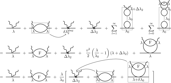
Figure 2: Diagrammatic renormalization of the $v^{2}$-dependent part of the self-energy. See the text for details. The symmetry factors are not indicated and we used the shorthand $\lambda_{0}=\lambda+\delta\lambda_{0}.$ The boxes denote the divergence of the encircled part of the graph, the plain line denotes the propagator $G^{\,\textrm{(v)}}(P)\equiv G_{0}(P),$ while “F” denotes the finite part of the bubble integral. The index $l$ in the sums goes over the possible number of bubbles (for the two classes of diagrams the lowest number of bubbles is zero or one, as indicated).

We close this subsection with a diagrammatic illustration of the renormalization of the part proportional to $v^{2}$ in Eq. (10b) for $\Sigma^{(0)},$ see Fig. 2. This is interesting because it shows the role the coupling counterterms play in the removal of both subdivergences and overall divergences. The first line in the figure shows the $v^{2}$-dependent diagrams generated upon iterating Eq. (10b) after the Bogoliubov-Parasiuk-Hepp-Zimmermann (BPHZ) subtraction procedure was implemented (see Berges:2005hc for details.) The counterterm $\delta\lambda_{2}$ displayed in Fig. 1 is decomposed in the sum of two terms $\delta\lambda_{2}^{\rm BPHZ}$ and $\Delta\lambda_{2},$ and $\delta\lambda_{2}^{\rm BPHZ}$ is used to absorb the divergence of the bubble integral present in $\Lambda_{2}^{(\rm v)}(0,P).$ The remaining finite part of the bubble integral is denoted by ’F’. In order to obtain the second line of the figure we localized all the subdivergences. Then, we used the renormalization condition (24). To obtain the third line of the figure, a cancellation occuring between the third and fourth term of the second line was exploited and the consequence of the renormalization condition (24), that is $\lambda-\lambda_{0}=(\lambda_{0}\lambda/2)\int_{K}G^{\,\textrm{(v)}}(K),$ where $\lambda_{0}=\lambda+\delta\lambda_{0},$ was rewritten in a diagrammatic form. The remaining overall divergences of the diagrams in the third line are removed by $\Delta\lambda_{2}.$ Since the divergent integrals associated with these diagrams are $T_{d}^{(0)}$ and $T_{d}^{(I)},$ keeping in mind that one has to add also $\delta\lambda_{2}^{\rm BPHZ},$ from the condition of vanishing of the square bracket in the last line of Fig. 2 one obtains the expression of $\delta\lambda_{2}$ determined previously.

III.2 Renormalization of the field equation in the broken symmetry phase

We use in the field equation (4) the splitting of the propagator introduced in the previous subsection in (8) and obtain

$$0 = m^{2}+\delta m_{0}^{2}+\frac{\lambda+\delta\lambda_{2}}{2}\int_{P}G^{\,\textrm{(v)}}(P)-i\frac{\lambda^{2}}{6}\int_{P}\int_{K}G^{\,\textrm{(v)}}(P+K)G^{\,\textrm{(v)}}(P)G^{\,\textrm{(v)}}(K)$$ (31)

$$+\frac{\lambda+\delta\lambda_{4}}{6}v^{2}+\frac{1}{2}\int_{K}\Lambda_{2}^{\textrm{(v)}}(0,K)G^{\,\textrm{(m)}}(K)-i\frac{\lambda^{2}}{6}\int_{P}\int_{K}\Big{(}3G^{\,\textrm{(v)}}(P)+G^{\,\textrm{(m)}}(P)\Big{)}G^{\,\textrm{(m)}}(P+K)G^{\,\textrm{(m)}}(K).$$

Using (13) and (17) in the second line, we obtain

$$0 = m^{2}+\delta m_{0}^{2}+\frac{\lambda+\delta\lambda_{2}}{2}\int_{P}G^{\,\textrm{(v)}}(P)-i\frac{\lambda^{2}}{6}\int_{P}\int_{K}G^{\,\textrm{(v)}}(P)G^{\,\textrm{(v)}}(P+K)G^{\,\textrm{(v)}}(K)$$ (32)

$$-\frac{i}{2}\Gamma_{m}^{\textrm{(v)}}\int_{K}\Lambda_{2}^{\textrm{(v)}}(0,K)\Big{(}G^{\,\textrm{(v)}}(K)\Big{)}^{2}+\frac{v^{2}}{6}\Gamma_{4}^{\textrm{(v)}}+\frac{1}{2}\int_{K}\Gamma_{2}^{\textrm{(v)}}(0,K)G^{\,\textrm{(r)}}(K)$$

$$-i\frac{\lambda^{2}}{6}\int_{P}\int_{K}\Big{(}3G^{\,\textrm{(v)}}(P)+G^{\,\textrm{(m)}}(P)\Big{)}G^{\,\textrm{(m)}}(P+K)G^{\,\textrm{(m)}}(K),$$

where we used the expression of $\Gamma_{2}^{\textrm{(v)}}$ given in (29) and defined

$$\Gamma_{4}^{\textrm{(v)}}=\lambda+\delta\lambda_{4}-\frac{3}{2}i\int_{K}\Lambda_{2}(0,K)\Big{(}G^{\,\textrm{(v)}}(K)\Big{)}^{2}\Gamma_{2}^{\textrm{(v)}}(0,K).$$ (33)

The integral in the expression above is divergent, and one imposes the following renormalization condition on $\Gamma_{4}^{\textrm{(v)}}:$

$$\Gamma_{4}^{\textrm{(v)}}=\lambda.$$ (34)

This leads to the equation for $\delta\lambda_{4}$ given in (66e).

Since the last but one term of (32) is already finite in view of (26) and (27), and the last term is a finite integral, we are left with the divergences of the first line and the first term of the second line. In order to complete the renormalization one only has to find the quantity on which the renormalization condition determining $\delta m_{0}^{2}$ can be imposed. It is straightforward to check that

$$\frac{\delta^{2}V[v,G_{v}]}{\delta v\delta v}\bigg{|}_{v=0}=m^{2}+\delta m_{0}^{2}+\frac{\lambda+\delta\lambda_{2}}{2}\int_{P}G_{v=0}(P)-i\frac{\lambda^{2}}{6}\int_{P}\int_{K}G_{v=0}(P+K)G_{v=0}(P)G_{v=0}(K),$$ (35)

where $G_{v}$ on the left-hand side is the solution of the stationarity condition $\delta V[v,G_{v}]/\delta G_{v}=0$ and the subscript indicates explicitly that it depends on the vacuum expectation value $v,$ so that the chain rule has to be applied when taking the derivatives with respect to $v.$ With the splitting of the propagator $G_{v=0}$ into vacuum, matter, and “regular” parts, one can proceed exactly as at the beginning of this subsection, only that one has to omit everywhere the $v$-dependent terms. Then, one has

$$\frac{\delta^{2}V[v,G_{v}]}{\delta v\delta v}\bigg{|}_{v=0} = m^{2}+\delta m_{0}^{2}+\frac{\lambda+\delta\lambda_{2}}{2}\int_{P}G^{\,\textrm{(v)}}(P)-i\frac{\lambda^{2}}{6}\int_{P}\int_{K}G^{\,\textrm{(v)}}(P)G^{\,\textrm{(v)}}(P+K)G^{\,\textrm{(v)}}(K)$$ (36)

$$-\frac{i}{2}\Gamma_{m}^{\textrm{(v)}}\int_{K}\Lambda_{2}^{\textrm{(v)}}(0,K)\Big{(}G^{\,\textrm{(v)}}(K)\Big{)}^{2}+\frac{1}{2}\int_{K}\Gamma_{2}^{\textrm{(v)}}(0,K)G^{\,\textrm{(r)}}_{v=0}(K)$$

$$-i\frac{\lambda^{2}}{6}\int_{P}\int_{K}\Big{(}3G^{\,\textrm{(v)}}_{v=0}(P)+G^{\,\textrm{(m)}}_{v=0}(P)\Big{)}G^{\,\textrm{(m)}}_{v=0}(P+K)G^{\,\textrm{(m)}}_{v=0}(K).$$

The last term above is finite and since $\Gamma_{2}^{\textrm{(v)}}(0,K)$ was already made finite by imposing the condition (26), the last but one term above is also finite. Therefore, one could in principle formulate our last renormalization condition as $\frac{\delta^{2}V[v,G_{v}]}{\delta v\delta v}\big{|}_{\textrm{v=0}}=m^{2},$ but then $\delta m_{0}^{2}$ determined through this condition would differ by a finite term from $\delta m_{0}^{2}$ given in (66d). In order to obtain the desired expression for $\delta m_{0}^{2}$ one choose the following condition

$$\frac{\delta^{2}V[v,G_{v}]}{\delta v\delta v}\bigg{|}_{\textrm{v=0, overall}}=m^{2},$$ (37)

where the concrete expression on the left-hand side is given by the right-hand side of (36) without the last two terms, and the overall notation indicates that the divergence of this term is the usual overall divergence, that is the divergence which remains after all subdivergences are removed. Then, it is easy to check that (37) gives indeed for $\delta m_{0}^{2}$ the expression in (66d).

The two renormalization conditions (33) and (66d) together with the expression of $\Gamma_{2}^{\textrm{(v)}}(0,K)$ given in (27) leads to the explicitly finite version of the field equation

$$0 = m^{2}+\frac{\lambda}{6}v^{2}+\frac{\lambda}{2}\int_{P}\Big{(}1+\lambda I_{F}^{\textrm{(v)}}(P)\Big{)}G^{\,\textrm{(r)}}(P)$$ (38)

$$-i\frac{\lambda^{2}}{2}\int_{P}\int_{K}G^{\,\textrm{(v)}}(P+K)G^{\,\textrm{(m)}}(P)G^{\,\textrm{(m)}}(K)-i\frac{\lambda^{2}}{6}\int_{P}\int_{K}G^{\,\textrm{(m)}}(P+K)G^{\,\textrm{(m)}}(P)G^{\,\textrm{(m)}}(K).$$

The renormalization conditions imposed above give exactly the same expressions for these counterterms introduced in the functional (2) as those appearing in patkos08 (see also [66)]. This demonstrates the equivalence between the two renormalization procedures. We note that even though we formulated our set of renormalization conditions on the quantities $\Gamma^{\textrm{(v)}},\Gamma_{2}^{\textrm{(v)}}(0,P),$ $\Gamma_{4}^{\textrm{(v)}}$, corresponding to the three four-point functions $\bar{V},$ $V(0,P)=\delta^{2}\Sigma(P)/\delta v^{2},$ $\hat{V}=\delta^{4}V[v,G_{v}]/\delta v^{4},$ introduced in Berges:2005hc , and also using the curvature $\delta^{2}V[v,G_{v}]/\delta v\delta v$, they do not look as natural as those imposed in Berges:2005hc ; arrizabalaga06 at $T=T^{*}$ and in the symmetric phase of the model ($v=0$). In our case $G^{\,\textrm{(v)}}$ is not the full propagator at $v=0$ and in order to obtain a given expression of the counterterms which contains $G^{\,\textrm{(v)}}$ in place of the full propagator we need a specific way to formulate the renormalization condition in (22) and (37). One may even say that some of our conditions used for renormalization are not genuine renormalization conditions because they are not formulated on quantities accessible from the effective potential through functional derivatives and resemble more the way divergences are removed in a minimal subtraction scheme. As we have already formulated, we imposed these conditions in order to facilitate the comparison, to be done in the next section, between the solution of the finite equations and those using counterterms. On the other hand, as discussed in Ref. Reinosa:2011ut , finding a set of natural renormalization condition, prescribing e.g. the mass defined from the variational propagator and the curvature at the minimum of the effective potential together with the value of the independent four-point functions is problematic when renormalizing the model at $T=0,$ that is in the broken symmetry phase, even at the Hartree level approximation of the 2PI effective potential.

IV Numerical implementation and results

Before discussing the algorithms and presenting the results we make some general statements about the numerical method used.

Since we solve iteratively the set of coupled integral equations consisting of the self-consistent propagator equation and the field equation, one has to store and upgrade in each iteration step the value of some functions on a grid and to approximate using interpolation the value of these functions at the points required by the integration routine. For this purpose we use an equidistant grid for the modulus of the four-momentum, the one-dimensional Akima spline interpolation method and the numerical integration routines of the GNU Scientific Library gsl . When we solve the set of finite equations, one stores the regular and the matter part of the propagator [see (13)], while when solving the set of equations with the counterterms it is the full self-energy which is stored on the grid [see (9 and (10)]. In the first case the integrals are convergent in the UV, but nevertheless, for the functions which are stored on the grid we have to take into account the fact that there is a maximal value of the modulus of the four-momentum. The convolution of these functions should be calculated accordingly, using $\theta$ functions to restrict the momenta of the propagators, see (60). For functions of the momentum with a known analytical expression there is no need to store them on the grid, and in consequence a simplification is encountered in the convolution involving such functions, see e.g. (62). In contradistinction to this, when counterterms are used, all momentum-dependent functions are cut at the maximal value of the modulus of the four-momenta, that is at the physical cutoff $\Lambda,$ irrespective of the fact that they are stored or not stored on the grid, in the latter case their expression is known analytically. We mention here that cutting the sum of momenta in the case of the bubble integral and as a consequence in all the double integrals encountered seems to be the cleanest way to proceed. In fact, in the case of solving the set of finite equations we could afford to simplify the calculation, by cutting only the loop momenta in the integrals involving the propagator $G^{\,\textrm{(v)}}(P)\equiv G_{0}(P)$ which is not stored on the grid, because the integrals are all convergent in the UV, and in consequence the corrections are suppressed. We will see indeed that the solution of the finite equations nicely agrees with that obtained by solving the equations with counterterms. Moreover, cutting only the loop-momenta, when solving the set of equation containing the counterterms, produces some small differences compared to the case when the sum of momenta is also cut, at least up to the largest cutoff we investigated, and in consequence is not a viable method for obtaining accurate numerical results.

IV.1 Algorithm for solving the finite propagator and field equations

We will solve in Euclidean space the explicitly finite field and propagator equations obtained in the previous section. A Wick rotation is performed in every integral appearing in our equations: for example with the continuation $k_{0}\to ik^{4}$ the tadpole integral reads $\int_{K}G(k_{0},{\bf k})\to i\int_{k_{E}}G(ik^{4},{\bf k})=\int_{k_{E}}\Delta(k_{E})$ where the Euclidean four-momenta is $k_{E}=({\bf k},k^{4})$, such that $k_{E}^{2}={\bf k}^{2}+k_{4}^{2}$ and the Euclidean propagator is defined as $\Delta(k_{E})=1/(k_{E}^{2}+\Sigma(k_{E})).$

Using the expansion (12) of the propagator around the vacuum propagator $\Delta^{\textrm{(v)}}(k_{E})=1/(k_{E}^{2}+M_{0}^{2})$ and the definition (13), the matter and regular parts of the Euclidean propagator reads

$$\Delta^{\textrm{(m)}}(k_{E}) = \frac{1}{k_{E}^{2}+M_{0}^{2}+\Sigma^{\textrm{(0)}}(k_{E})+\Sigma^{\textrm{(r)}}(k_{E})}-\frac{1}{k_{E}^{2}+M_{0}^{2}},$$ (39)

$$\Delta^{\textrm{(r)}}(k_{E}) = \Delta^{\textrm{(m)}}(k_{E})+\frac{\Sigma^{\textrm{(0)}}(k_{E})}{(k_{E}^{2}+M_{0}^{2})^{2}}.$$ (40)

The two pieces of the self-energy which appear above are given by

$$\Sigma^{\textrm{(0)}}(k_{E}) = m^{2}-M_{0}^{2}+\lambda\Big{(}1+\lambda I_{F}^{\textrm{(v)}}(k_{E})\Big{)}\frac{v^{2}}{2}+\frac{\lambda}{2}\int_{k_{E}}\Delta^{\textrm{(r)}}(k_{E}),$$ (41)

$$\Sigma^{\textrm{(r)}}(k_{E}) = \lambda^{2}v^{2}I^{\textrm{(mv)}}(k_{E})+\frac{\lambda^{2}v^{2}}{2}I^{\textrm{(mm)}}(k_{E}),$$ (42)

where the “matter-vacuum” and “matter-matter” bubble integrals are defined as

$$I^{\textrm{(mv)}}(k_{E}) = -\int_{p_{E}}\Delta^{\textrm{(m)}}(p_{E})\Delta^{\textrm{(v)}}(p_{E}+k_{E}),$$ (43a)

$$I^{\textrm{(mm)}}(k_{E}) = -\int_{p_{E}}\Delta^{\textrm{(m)}}(p_{E})\Delta^{\textrm{(m)}}(p_{E}+k_{E}).$$ (43b)

The finite part of the vacuum bubble integral, $I_{F}^{\textrm{(v)}}$, appearing in (41), is defined in (68). After analytical continuation to Euclidean space it has the following expression (recall that $G_{0}\equiv G^{\,\textrm{(v)}}$):

$$I_{F}^{\textrm{(v)}}(k_{E})=\frac{1}{16\pi^{2}}\Bigg{[}\sqrt{1+\frac{4M_{0}^{2}}{k_{E}^{2}}}\ln\frac{\sqrt{1+\frac{4M_{0}^{2}}{k_{E}^{2}}}+1}{\sqrt{1+\frac{4M_{0}^{2}}{k_{E}^{2}}}-1}-2\Bigg{]}.$$ (44)

Note that a self-consistent equation for the regular part $\Delta^{\textrm{(r)}}$ can be obtained in principle if one substitutes the expression of $\Delta^{\textrm{(m)}}$ from (39) into (40) because $\Sigma^{\textrm{(0)}}$ contains the integral of $\Delta^{\textrm{(r)}}$ and $\Delta^{\textrm{(m)}}$ appearing in the integrals of $\Sigma^{\textrm{(r)}}$ can be expressed in terms of $\Delta^{\textrm{(r)}}$ and $\Sigma^{\textrm{(0)}}.$ Nevertheless, we store on the grid two quantities, $\Delta^{\textrm{(m)}}$ and $\Delta^{\textrm{(r)}},$ which have to be solved simultaneously with the field equation (38), which in Euclidean space reads

$$0=m^{2}+\frac{\lambda}{6}v^{2}+\frac{\lambda}{2}\int_{k_{E}}\Big{(}1+\lambda I_{F}^{\textrm{(v)}}(k_{E})\Big{)}\Delta^{\textrm{(r)}}(k_{E})+\frac{\lambda^{2}}{6}\big{(}3S^{\textrm{(mmv)}}+S^{\textrm{(mmm)}}\big{)},\\$$ (45)

where the corresponding pieces of the setting-sun integral are defined as

$$S^{\textrm{(mmv)}} = -\int_{p_{E}}\int_{k_{E}}\Delta^{\textrm{(m)}}(p_{E})\Delta^{\textrm{(m)}}(k_{E})\Delta^{\textrm{(v)}}(p_{E}+k_{E}),$$ (46a)

$$S^{\textrm{(mmm)}} = -\int_{p_{E}}\int_{k_{E}}\Delta^{\textrm{(m)}}(p_{E})\Delta^{\textrm{(m)}}(k_{E})\Delta^{\textrm{(m)}}(p_{E}+k_{E}).$$ (46b)

Our iterative algorithm for solving the coupled set of equations for $\Delta^{\textrm{(r)}},$ $\Delta^{\textrm{(m)}},$ and $v$ goes as follows. One starts at zeroth order by neglecting all the integrals in the self-energy and the field equation, including the finite part of the bubble $I_{F}^{\textrm{(v)}}.$ By doing so, from (45), (39), and (40) one obtains:

$$v_{0}=\sqrt{-\frac{6m^{2}}{\lambda}},\ \ \quad\Delta^{\textrm{(m)}}_{0}(k_{E})=-\frac{m^{2}+\frac{\lambda}{2}v^{2}-M_{0}^{2}}{(k_{E}^{2}+M_{0}^{2})(k_{E}^{2}+m^{2}+\frac{\lambda}{2}v^{2})},\ \ \quad\Delta^{\textrm{(r)}}_{0}(k_{E})=\frac{\left(m^{2}+\frac{\lambda}{2}v^{2}-M_{0}^{2}\right)^{2}}{(k_{E}^{2}+M_{0}^{2})^{2}(k_{E}^{2}+m^{2}+\frac{\lambda}{2}v^{2})}.$$

Then, starting from the first order, the iteration is done in two steps. At a generic order $n\geq 1$ one first upgrades on the grid $\Delta^{\textrm{(m)}}_{n}$ and $\Delta^{\textrm{(r)}}_{n}$ using (39) and (40), respectively, where the self-energy, which includes now $I_{F}^{\textrm{(v)}},$ is calculated with the lower order quantities: $v_{n-1},$ $\Delta^{\textrm{(m)}}_{n-1},$ $\Delta^{\textrm{(r)}}_{n-1}.$ As a second step of the nth iteration, one upgrades the vacuum expectation value by calculating $v_{n}$ from (45) with the integrals done with the already upgraded $\Delta^{\textrm{(m)}}_{n}$ and $\Delta^{\textrm{(r)}}_{n}.$ This procedure is repeated until the iteration converges. The angular integration in the integrals appearing in (42) and (45) are performed in Appendix A as outlined at the beginning of this section.

IV.2 Algorithm for solving the propagator and field equations using counterterms

If one decides to solve the propagator and field equations using counterterms, whose role in this equations is to cancel the divergent part of the integrals, then one needs a method to determine them. Such a method was developed in patkos08 , and we review it here because it will be slightly modified for numerical reasons. In terms of the remaining finite part of the tadpole $T_{\rm F}[G]$ and bubble integral $I_{\rm F}(P,G)$ the propagator equation (3) reads

$$iG^{-1}(P)=P^{2}-M^{2}-\frac{1}{2}\lambda^{2}v^{2}I_{\rm F}(P,G),\qquad M^{2}=m^{2}+\frac{\lambda}{2}v^{2}+\frac{\lambda}{2}T_{\rm F}[G].$$ (47)

Using the expansion of $G$ around $G_{0}$

$$G(P)=G_{0}(P)-iG_{0}^{2}(P)\left(M^{2}-M_{0}^{2}+\frac{1}{2}\lambda^{2}v^{2}I_{\rm F}(P,G)\right)+\dots\,,$$ (48)

the tadpole, bubble, and setting-sun integrals can be explicitly decomposed into divergent and finite parts (see Ref. patkos08 for details):

$$I(P,G) = T_{d}^{(0)}+I_{\rm F}(P,G),$$ (49a)

$$T[G] = T_{d}^{(2)}+(M^{2}-M_{0}^{2})T_{d}^{(0)}+\frac{1}{2}\lambda^{2}v^{2}T_{d}^{(I)}+T_{\rm F}[G],$$ (49b)

$$S(0,G) = S_{0}(0)+3T_{d}^{(0)}T_{\rm F}[G]+3(M^{2}-M_{0}^{2})\left(\big{(}T_{d}^{(0)}\big{)}^{2}+T_{d}^{(I)}\right)+\frac{3}{2}\lambda^{2}v^{2}\left(T_{d}^{(I)}T_{d}^{(0)}+T_{d}^{(I,2)}\right)+S_{\rm F}(0,G),$$ (49c)

where the divergent integrals $T_{d}^{(2)},T_{d}^{(0)},T_{d}^{(I)},T_{d}^{(I,2)}$ and $S_{0}(0)$ are defined and calculated in Appendix B. Plugging the decomposed expressions of the integrals (49) into the propagator and field equations and subtracting from them the corresponding explicitly finite equations, written in terms of the renormalized parameters $m^{2},\lambda$ and the finite part of the integrals, one obtains relations between the counterterms and the divergent integrals. Requiring that the coefficient of the $v^{2},$ $v^{0},$ and $T_{F}[G]$ vanish independently, one obtains the counterterms determined in patkos08 . These were also obtained from appropriate renormalization conditions in Sec. III and are summarized in Appendix B.

In Euclidean space these counterterms are functions of the four-dimensional rotational invariant cutoff $\Lambda$ appearing through the integrals explicitly calculated in (70). They can be used to solve iteratively the set of Euclidean equations

$$\Sigma(p) = m^{2}+\delta m_{2}^{2}+\frac{1}{2}(\lambda+\delta\lambda_{2})v^{2}+\frac{1}{2}(\lambda+\delta\lambda_{0})T(\Sigma)+\frac{1}{2}\lambda^{2}v^{2}I(p,\Sigma),$$ (50a)

$$0 = m^{2}+\delta m_{0}^{2}+\frac{1}{6}(\lambda+\delta\lambda_{4})v^{2}+\frac{1}{2}(\lambda+\delta\lambda_{2})T(\Sigma)+\frac{\lambda^{2}}{6}S(0,\Sigma).$$ (50b)

However, since the counterterms determined from (66) are designed to cancel in these equations the divergences of integrals produced by the full (i.e. iteratively converged) propagator, they cancel the complete cutoff dependence of $T[\Sigma],$ $I(P,\Sigma)$ and $S(0,\Sigma)$ only when the solution of this set of equations has converged. This is not a problem in itself, since, as it will be demonstrated, the iterative procedure converges, but the convergence of the solution of the set of equations is rather slow. It is possible to improve the iterative procedure if, instead of using the counterterms given in (66), we rederive them at each order of the iteration using the procedure outlined above. These counterterms, which come from the requirement to have finite equations at each order of the iteration, will evolve during the process of iteration toward the value of the counterterms obtained from (66) which will be reached when the iteration converged. Since, as we will see, the new counterterms are now environment dependent, that is depend on $v$ and $T_{F}[\Sigma]$, this convergence can only happen if $v$ and $\Sigma$ also converge to their appropriate values, and has to be checked numerically.

In what follows we present the improved iterative procedure which uses evolving counterterms. At each order the iteration starts by the upgrade of the self-energy, followed by the upgrade of the vacuum expectation value determined from the field equation.

At zeroth order of the iteration the field and the self-energy are the tree-level ones:

$$v_{0}^{2}=-\frac{6m^{2}}{\lambda},\qquad\Sigma_{0}(p)=m^{2}+\frac{\lambda}{2}v_{0}^{2}.$$ (51)

At this order, since there are no quantum fluctuations at all, there are no divergences to cancel and in consequence all the counterterms are zero, that is $\delta m_{0,0}^{2}=\delta m_{2,0}^{2}=\delta\lambda_{0,0}=\delta\lambda_{2,0}=\delta\lambda_{4,0}=0,$ where the counterterms also carry the index of the iteration number because all of them will change during the iteration process.

The general formulas for the nth order counterterms to be given below encompass all orders with the following prescription: at $n=0$ one starts from the tree-level values, and formally $T(\Sigma_{n})=I(\Sigma_{n})=0$ for $n\in\{-1,-2\}$ and $v_{-1}=v_{0}.$ Suppose that the (n-1)th order of the iteration is done, i.e. $v_{n-1}^{2}$ and $\Sigma_{n-1}(p)$ together with the corresponding counterterms are already known, then at nth order we start by upgrading the self-energy using [c.f. (50a)]:

$$\Sigma_{n}(p)=m^{2}+\delta m_{2,n}^{2}+\frac{\lambda}{2}v_{n-1}^{2}+\frac{\delta\lambda_{2,n}}{2}v_{n-2}^{2}+\frac{\lambda+\delta\lambda_{0,n}}{2}T(\Sigma_{n-1})+\frac{\lambda^{2}}{2}v_{n-1}^{2}I(p,\Sigma_{n-1}).$$ (52)

The finite part of the tadpole and bubble are defined through

$$T(\Sigma_{n-1}) = T_{d}^{(2)}+\Big{(}m^{2}+\frac{\lambda}{2}v_{n-2}^{2}+\frac{\lambda}{2}T_{F}(\Sigma_{n-2})-M_{0}^{2}\Big{)}T_{d}^{(0)}+\frac{\lambda^{2}v_{n-2}^{2}}{2}T_{d}^{(I)}+T_{F}(\Sigma_{n-1}),$$ (53)

$$I(p,\Sigma_{n-1}) = T_{d}^{(0)}+I_{F}(p,\Sigma_{n-1}).$$ (54)

The renormalization procedure requires the independent vanishing of the overall divergence, field-dependent subdivergence and $T_{F}$-dependent subdivergence:

$$0 = \delta m_{2,n}^{2}+\frac{\lambda+\delta\lambda_{0,n}}{2}\Big{(}T_{d}^{(2)}+(m^{2}-M_{0}^{2})T_{d}^{(0)}\Big{)},$$ (55a)

$$0 = \delta\lambda_{2,n}+\frac{\lambda}{2}T_{d}^{(0)}(\lambda+\delta\lambda_{0,n})+\frac{\lambda^{2}}{2}T_{d}^{(I)}(\lambda+\delta\lambda_{0,n})(1-\delta_{n,1})+\lambda^{2}T_{d}^{(0)}\frac{v_{n-1}^{2}}{v_{n-2}^{2}},$$ (55b)

$$0 = (\lambda+\delta\lambda_{0,n})\frac{\lambda}{2}T_{d}^{(0)}T_{F}(\Sigma_{n-2})+\delta\lambda_{0,n}T_{F}(\Sigma_{n-1}).$$ (55c)

The counterterms $\delta m_{2,n}^{2}$, $\delta\lambda_{2,n}$ and $\delta\lambda_{0,n}$ are obtained from (55), so that $\Sigma_{n}(p)$ is finite and can be calculated. Note that for $n=1$ the second term in the equation for $\delta\lambda_{2,n}$ vanishes as it should because in this case there is no divergence due to the bubble, that is there is no $T_{d}^{(I)}$ in $T(\Sigma_{0})$, whose expression is

$$T(\Sigma_{0})=T_{d}^{(2)}+\Big{(}m^{2}+\frac{\lambda}{2}v_{0}^{2}-M_{0}^{2}\Big{)}T_{d}^{(0)}+T_{F}(\Sigma_{0}).$$ (56)

Note also that for $n=1$ one has $\delta\lambda_{0,1}=0$, since $T_{F}(\Sigma_{-1})=0$ by convention.

We continue with the determination of $v_{n}^{2}$ from the field equation, which at nth order of the iteration reads

$$0 = m^{2}+\delta m_{0,n}^{2}+\frac{\lambda}{6}v_{n}^{2}+\frac{\delta\lambda_{4,n}}{6}v_{n-1}^{2}+\frac{\lambda+\delta\tilde{\lambda}_{2,n}}{6}T(\Sigma_{n})+\frac{\lambda^{2}}{6}S(0,\Sigma_{n}),$$ (57)

where $T(\Sigma_{n})$ is given by (53) with $n-1\to n$ and the setting sun is

$$S(0,\Sigma_{n}) = S_{0}(0)+3T_{d}^{(0)}T_{\rm F}[\Sigma_{n}]+3\Big{(}m^{2}+\frac{\lambda}{2}v_{n-1}^{2}+\frac{\lambda}{2}T_{F}(\Sigma_{n-1})-M_{0}^{2}\Big{)}\left(\big{(}T_{d}^{(0)}\big{)}^{2}+T_{d}^{(I)}\right)$$ (58)

$$+\frac{3}{2}\lambda^{2}v^{2}_{n-1}\left(T_{d}^{(I)}T_{d}^{(0)}+T_{d}^{(I,2)}\right)+S_{\rm F}(0,\Sigma_{n}).$$

Applying the same requirements as for the self-energy, one obtains:

$$0 = \delta m_{0,n}^{2}+\frac{\lambda+\delta\tilde{\lambda}_{2,n}}{2}\Big{(}T_{d}^{(2)}+(m^{2}-M_{0}^{2})T_{d}^{(0)}\Big{)}+\frac{\lambda^{2}}{2}(m^{2}-M_{0}^{2})\Big{(}(T_{d}^{(0)})^{2}+T_{d}^{(I)}\Big{)}+\frac{\lambda^{2}}{6}S_{0}(0),\quad$$ (59a)

$$0 = \delta\lambda_{4,n}+\frac{3\lambda}{2}(\lambda+\delta\tilde{\lambda}_{2,n}+\lambda^{2}T_{d}^{(0)})\Big{(}T_{d}^{(0)}+\lambda T_{d}^{(I)}\Big{)}+\frac{3\lambda^{3}}{2}\Big{(}T_{d}^{(I)}+\lambda T_{d}^{(I,2)}\Big{)},$$ (59b)

$$0 = \delta\tilde{\lambda}_{2,n}+\lambda^{2}T_{d}^{(0)}+\frac{T_{F}(\Sigma_{n-1})}{T_{F}(\Sigma_{n})}\Big{[}\frac{\lambda}{2}(\lambda+\delta\tilde{\lambda}_{2,n})T_{d}^{(0)}+\frac{\lambda^{3}}{2}\Big{(}(T_{d}^{(0)})^{2}+T_{d}^{(I)}\Big{)}\Big{]}.$$ (59c)

Note that a new counterterm $\delta\tilde{\lambda}_{2}$ has been introduced instead of $\delta\lambda_{2}$, since in the $n$th iteration $\delta\lambda_{2,n}$ does not eliminate properly the appropriate subdivergences of the field equation. Extracting $\delta m_{0,n}^{2}$, $\delta\lambda_{4,n}$ and $\delta\tilde{\lambda}_{2,n}$, from (59) one can obtain $v_{n}^{2}$ from (57). The counterterm $\delta\tilde{\lambda}_{2,n}$ will be equal to $\delta\lambda_{2,n}$ determined from the propagator equation only when the iteration converged, so that $T_{F}(\Sigma_{n-1})/T_{F}(\Sigma_{n})\to 1.$ In this limit and when $v_{n}/v_{n-1}\to 1$ the counterterms will converge to the values obtained from (66). This happens only asymptotically and in practice the iteration stops when the relative change in the values of the field and the self-energy are smaller than some given value dictated by our requirement of accuracy. The same iterative procedure is used when the counterterms are not evolved during the iteration, but used as determined from (66): one first upgrades the self-energy and then the field equation and checks for their convergence.

IV.3 Numerical results

In what follows we present the results on the numerical solution of the propagator and field equations in Euclidean space. When solving the explicitly finite set of equations the maximal value of the modulus of the four-momentum stored on the grid is $L/\sqrt{2|m^{2}|}=500,$ while in the case of solving equations with counterterms the highest value of the modulus stored, that is the four-dimensional physical cutoff, is $\Lambda/\sqrt{2|m^{2}|}=200.$ The value of the mass scale is chosen to be $M_{0}/\sqrt{2|m^{2}|}=2.1$ and the value of the renormalized mass parameter squared is $m^{2}=-0.5,$ in some arbitrary physical units. Actually, to have an idea on the physical scale, one can require to have $v/\Sigma^{\frac{1}{2}}(p=0)\simeq 0.66,$ which is the value of the ratio $f_{\pi}/m_{\pi}$ of the pion decay constant to the pion mass for $f_{\pi}=93$ MeV and $m_{\pi}=140$ MeV, and $\Sigma^{\frac{1}{2}}(p=0)=m_{\pi}.$ Then, from the left panel of Fig. 3 one sees that the first condition can be meet by choosing $\lambda\simeq 8,$ for which value the second condition means $\sqrt{2|m^{2}|}\simeq 158$ MeV. In units for which $m^{2}=-0.5$ the step size on the grid in general was $0.01.$ We have checked that by halving the step size the change in the results is comparable with or smaller than the precision required by our convergence criterion. The iteration was stopped when the change in the vacuum expectation value was smaller than $10^{-6}.$ The precision of the numerical integration routines used was higher than that, since we required relative error bounds between $10^{-6}$ and $10^{-8}$.

Figure 3: The solution of the explicitly finite propagator and field equations. Left panel: $v/M$ and $M=\Sigma^{\frac{1}{2}}(p=0)$ as function of the coupling obtained for $L/\sqrt{2|m^{2}|}=500$. Right panel: The converged value of $v$ as function of the maximal value of the modulus of the momentum stored on the grid for different values of the coupling constant $\lambda$. An appropriate constant was subtracted from the values of $v$ obtained for $\lambda=3,$ $10,$ and $20$ such that the resulting values coincide at $L/\sqrt{2|m^{2}|}=500$ with the value of $v$ obtained for $\lambda=30.$

The solution of the explicitly finite equations can be seen in Fig. 3. In the right panel one can see the converged solution of the field equation obtained for various values of the coupling as function of $L,$ the maximal value of the modulus stored on the grid. As explained in the figure caption, $v$ was shifted appropriately in order to make all four curves meet at $L/\sqrt{2|m^{2}|}=500.$ In all cases a plateau can be observed for increasing values of $L.$ However, with increasing value of the coupling $\lambda$ the plateau starts at a higher $L.$ With the same convergence criterion the number of iterations increases with increasing $\lambda$ and for $\lambda=30$ one needs twice as many iterations until convergence occurs compared to the $\lambda=3$ case. Interestingly, at a given $\lambda,$ the number of iterations does not depend on $L.$

Figure 4: A comparison between the convergence of the iterative algorithms using fixed and evolving counterterms for a fix value of the physical cutoff: $\Lambda/\sqrt{2|m^{2}|}=200.$ The value of $v/\sqrt{2|m^{2}|}$ is shown as function of the number of iterations for different values of the coupling.

Next, we would like to quantify the extent of achievable improvement given by the use of the iteratively evolved coupling and mass counterterms, as compared to the solution of the equations which use the counterterms originally derived in patkos08 . In these two cases we compare in Fig. 4 the number of iterations needed for the convergence of $v$ at four different coupling constants. We use a reasonably large cutoff $\Lambda/\sqrt{2|m^{2}|}=200$, around which the convergent results are expected to show cutoff independence within some desired accuracy. One observes the advantage of evolving the counterterms even for lower values of the renormalized coupling. For larger values ($\lambda\gtrsim 10$) the improvement is significant, as one can see from the large iteration number needed by the algorithm using fixed counterterms. Therefore, it is expected in general that solving self-consistent equations iteratively in a fully nonperturbative regime with fixed counterterms is not efficient from a numerical point of view. For large couplings, $\lambda\gtrsim 10,$ the number of iterations needed in case of using fixed counterterms are at least a factor of 2 larger than the number of iterations needed for the explicitly finite equations to converge.

Figure 5: A comparison between the convergence rate of the iterative algorithms using fixed (left panel) and evolving counterterms (right panel) as reflected in the change of the vacuum expectation value at different values of the physical cutoff $\Lambda$. The horizontal line represents the solution of the explicitly finite system of equations obtained with $L/\sqrt{2|m^{2}|}=500,$ where $L$ is the maximal value of the modulus of the momentum stored on the grid. The insets show the convergence at large iteration numbers.

In Fig. 5 we compare for $\lambda=5$ the ways how a cutoff independent solution is reached using fixed and evolving counterterms. The left panel shows that with increasing values of $\Lambda$ a plateau in the $v(\Lambda)$ functions is approached rather slowly when the fixed counterterms of patkos08 are used, despite the fact that the coupling is not large. Looking at the plot with values of $\Lambda$ spanning a large range it seams that after several iterations a plateau is finally reached. However, the structure in $v(\Lambda),$ better seen in the inset which uses a smaller $\Lambda$ range, shows that the convergence is not uniform: more iterations are needed for larger cutoffs to get close to the true solution, that is the solution of the explicitly finite equations (horizontal line). This nonuniformity of the convergence in $\Lambda$ is more pronounced for larger values of the coupling constant. Contrary to this, the right panel of Fig. 5 shows a uniform convergence in $\Lambda$ when the iterative algorithm uses evolving counterterms. Since by the very construction of the evolving counterterms a plateau is observed already for moderate values of the cutoff at every order of the iteration, one sees again that with this improved approach the final, convergent result is obtained in a more efficient way.

The convergence of the self-energy can be seen in Fig. 6. The function converges smoothly, i.e. for all momentum values the self-energy reaches its converged value almost simultaneously. Note however that the convergence for $p_{E}\simeq 0$ is slightly slower as compared to larger values of the momenta.

Figure 6: The convergence of the full self-energy obtained for $\lambda=5$ with evolving counterterms for $\Lambda/\sqrt{2|m^{2}|}=200.$ The inset shows the behavior of the self-energy at large momenta.

V Conclusions

We presented an approach which can be used to obtain a very accurate numerical solution of the self-consistent propagator equation coupled to the field equation, both derived from the two-loop level approximation of the 2PI effective action in the $\phi^{4}$ model. We showed that the renormalization method developed in patkos08 which removes the divergences using minimal subtraction is equivalent to imposing nontrivial renormalization conditions on the self-energy, the curvature of the effective potential and on kernels of Bethe-Salpeter equations related to these quantities. The use of renormalization conditions also allowed us to construct explicitly finite propagator and field equations.

We compared the convergence of the iterative method applied to solve, on the one hand, the explicitly finite equations and, on the other hand, the equations which contains the explicitly calculated counterterms of patkos08 . The very same results were obtained numerically which indicates the correctness of our analytic study on renormalization. It turned out that, especially for larger coupling constants ($\lambda\gtrsim 10$), the convergence rate of the algorithm which uses the counterterms is quite poor. This should not come as a surprise given that the counterterms were determined based on the asymptotic behavior of the propagator. Within an iterative procedure the asymptotics develops progressively and is reached only when the solution converged. Only then the divergences present in the equations match the counterterms constructed to cancel them, at intermediate steps of the iteration process the use of fixed counterterms results in an oversubtraction. In order to cure this, we managed to develop a different algorithm which rederives the counterterms at every step of the iterative procedure from the condition that the counterterms cancel the divergent part of the integrals at every order of the iteration. This method which uses evolving counterterms turned out to be very effective in obtaining the converged solution within a few iterative steps also for larger couplings.

The presented approach and some of the methods applied in our present work may be directly extended, first to a zero temperature numerical solution of the model in Minkowski space, and then to a finite temperature solution of the model, where it would be interesting to investigate the order of the phase transition. We expect that the solution which can be obtained with the method described here could serve as a good benchmark for other, even more effective methods used in finite temperature studies (see e.g. Berges:2004hn ; arrizabalaga06 ). Some of these investigations will be presented in forthcoming publications. We expect that our methods presented here will represent a good basis for obtaining highly accurate and/or numerically controlled solutions of the 2PI approximation in more complicated theories as well. We plan to carry out the study of the phase transition in the $O(N)$ symmetric model using large-$N$ expansion. This is motivated by the fact that properly renormalized complete solutions of the equations derived in the $O(N)$ model at next-to-leading order of the 2PI-$1/N$ expansion are missing from the literature. The renormalization and the thermodynamics of the $O(N)$ model was investigated recently at the next-to leading order of the 1PI-$1/N$ expansion in Andersen:2008qk .

Appendix A Integrals appearing in the finite Euclidean equations

Since the functions appearing in the quantum correction integrals depend only on the modulus of the four-momentum, certain parts of the angular integral and in some cases the entire angular integral can be performed analytically. The angular integration for the integrals involving $\Delta^{\textrm{(r)}}$ is trivial, while the integral over the modulus of the four-momentum can be performed only numerically. As explained at the beginning of Sec. IV for the convolution of two functions stored on a grid one uses

$$C_{L}[f,g](k_{E}) = \int\frac{d^{4}p_{E}}{(2\pi)^{4}}f(|p_{E}|)g(|p_{E}+k_{E}|)\theta(L-|k_{E}|)\theta(L-|k_{E}+p_{E}|)$$ (60)

$$= \frac{1}{8\pi^{3}k_{E}^{2}}\int_{0}^{L}dp\,p\,f(p)\int_{|p-|k_{E}||}^{\textrm{min}(p+|k_{E}|,L)}dq\,q\,g(q)\sqrt{4p^{2}q^{2}-\big{(}p^{2}+q^{2}-k_{E}^{2}\big{)}^{2}},$$

where $\theta$ is the step function, and for the modulus we introduced $p=|p_{E}|,$ $q=|k_{E}+p_{E}|,$ $L$ is the maximal value of the modulus stored on the grid. The $q$ integral is a remnant of the angular integration in a four-dimensional spherical coordinate system and is obtained with the change of variable $\cos\theta_{1}=(q^{2}-k^{2}-p^{2})/(2kp).$ When the function $g$ is $\Delta^{\textrm{(v)}},$ which is not stored on the grid, that is there is no need for the second $\theta$ function, the entire angular integration can be done analytically, and with the change of variable $t=\tan(\theta_{1}/2)$ one has

$$\int_{0}^{\pi}d\theta_{1}\frac{\sin^{2}\theta_{1}}{p_{E}^{2}+k_{E}^{2}+2|p_{E}|\,|k_{E}|\cos\theta_{1}+M_{0}^{2}}=\frac{\pi}{4k_{E}^{2}p_{E}^{2}}\left(k_{E}^{2}+p_{E}^{2}+M_{0}^{2}-\sqrt{\big{(}k_{E}^{2}+p_{E}^{2}+M_{0}^{2}\big{)}^{2}-4k_{E}^{2}p_{E}^{2}}\right).$$ (61)

Using (61) in the first term of (42) and for the setting-sun contribution to the field equation (45) which contains one vacuum propagator one obtains

$$I^{\textrm{(mv)}}(k_{E}) = -\frac{1}{16\pi^{2}k_{E}^{2}}\int_{0}^{L}dp\,p\left(k_{E}^{2}+p^{2}+M_{0}^{2}-\sqrt{\big{(}k_{E}^{2}+p^{2}+M_{0}^{2}\big{)}^{2}-4k_{E}^{2}p^{2}}\right)\Delta^{\textrm{(m)}}(p),$$ (62)

$$S^{\textrm{(mmv)}} = -\frac{1}{128\pi^{4}}\int_{0}^{L}dk\,k\,\Delta^{\textrm{(m)}}(k)\int_{0}^{L}dp\,p\left(k^{2}+p^{2}+M_{0}^{2}-\sqrt{\big{(}k^{2}+p^{2}+M_{0}^{2}\big{)}^{2}-4k^{2}p^{2}}\right)\Delta^{\textrm{(m)}}(p).\ \$$ (63)

For the second term of (42) and the setting-sun contribution to (45) which contains only matter propagators one uses (60) and the results of the angular integrations are

$$I^{\textrm{(mm)}}(k_{E}) = -\frac{1}{8\pi^{3}k_{E}^{2}}\int_{0}^{L}dp\,p\,\Delta^{\textrm{(m)}}(p)\int_{|p-|k_{E}||}^{\textrm{min}(p+|k_{E}|,L)}dq\,q\,\sqrt{4p^{2}q^{2}-\big{(}p^{2}+q^{2}-k_{E}^{2}\big{)}^{2}}\Delta^{\textrm{(m)}}(q),$$ (64)

$$S^{\textrm{(mmm)}} = -\frac{1}{64\pi^{5}}\int_{0}^{L}dk\,k\,\Delta^{\textrm{(m)}}(k)\int_{0}^{L}dp\,p\,\Delta^{\textrm{(m)}}(p)\int_{|p-k|}^{\textrm{min}(p+k,L)}dq\,q\sqrt{4p^{2}q^{2}-(p^{2}+q^{2}-k^{2})^{2}}\Delta^{\textrm{(m)}}(q).\ \ \$$ (65)

Appendix B Cutoff dependence of divergent integrals

For reader’s convenience we summarize below the equations for the counterterms obtained in patkos08 and rederived in Sec. III by imposing appropriate renormalization conditions:

$$0= \delta m_{2}^{2}+\frac{1}{2}(\lambda+\delta\lambda_{0})\left[T_{d}^{(2)}+(m^{2}-M_{0}^{2})T_{d}^{(0)}\right],$$ (66a)

$$0= \delta\lambda_{0}+\frac{1}{2}\lambda(\lambda+\delta\lambda_{0})T_{d}^{(0)},$$ (66b)

$$0= \delta\lambda_{2}+\frac{1}{2}\lambda(\lambda+\delta\lambda_{0})\left(T_{d}^{(0)}+\lambda T_{d}^{(I)}\right)+\lambda^{2}T_{d}^{(0)},$$ (66c)

$$0= \delta m^{2}_{0}+\frac{1}{2}(\lambda+\delta\lambda_{2})\left[T_{d}^{(2)}+(m^{2}-M_{0}^{2})T_{d}^{(0)}\right]+\frac{1}{2}\lambda^{2}(m^{2}-M_{0}^{2})\left((T_{d}^{(0)})^{2}+T_{d}^{(I)}\right)+\frac{1}{6}\lambda^{2}S_{0}(0),$$ (66d)

$$0= \delta\lambda_{4}+\frac{3}{2}\lambda(\lambda+\delta\lambda_{2}+\lambda^{2}T_{d}^{(0)})\left(T_{d}^{(0)}+\lambda T_{d}^{(I)}\right)+\frac{3}{2}\lambda^{3}\left(T_{d}^{(I)}+\lambda T_{d}^{(I,2)}\right).$$ (66e)

The first three and the last two expressions come from the renormalization of the propagator equation and field equation, respectively. The divergent quantities $T_{d}^{(2)},$ $T_{d}^{(0)},$ and $S_{0}(0)$ are the vacuum parts of the tadpole integral (6a), the bubble integral (6b) at vanishing external momentum and the setting-sun integral (6c), all calculated with the propagator $G_{0}$ given in (7):

$$T_{d}^{(2)} = \int_{P}G_{0}(P),$$ (67a)

$$T_{d}^{(0)} = \frac{dT_{d}^{(2)}}{dM_{0}^{2}}=-i\int_{P}G_{0}^{2}(P),$$ (67b)

$$S_{0}(0) = -i\int_{K}\int_{Q}G_{0}(K)G_{0}(Q)G_{0}(K+Q).$$ (67c)

The remaining two divergent integrals $T_{d}^{(I)}$ and $T_{d}^{(I,2)}$ are defined in terms of the finite part of the bubble integral (6b) calculated with the propagator $G_{0},$ that is

$$I_{0,F}(K)=-i\int_{P}\Big{(}G_{0}(P)G_{0}(P+K)-G_{0}^{2}(P)\Big{)}.$$ (68)

and read

$$T_{d}^{(I)} = -i\int_{K}G_{0}^{2}(K)I_{0,F}(K)=-i\int_{K}G_{0}^{2}(K)I_{0}(K)-\big{(}T_{d}^{(0)}\big{)}^{2},$$ (69a)

$$T_{d}^{(I,2)} = -i\int_{K}G_{0}^{2}(K)I_{0,F}^{2}(K)=-i\int_{K}G^{2}_{0}(K)I^{2}_{0}(K)-2T_{d}^{(I)}T_{d}^{(0)}-\big{(}T_{d}^{(0)}\big{)}^{3}.$$ (69b)

With a four-dimensional rotational invariant cutoff regularization in Euclidean space, the divergent integrals are computed as follows

$$T_{d}^{(2)} = \frac{\Lambda^{2}}{16\pi^{2}}\left[1-\frac{M_{0}^{2}}{\Lambda^{2}}\log\left(1+\frac{\Lambda^{2}}{M_{0}^{2}}\right)\right],\quad T_{d}^{(0)}=\frac{1}{16\pi^{2}}\left[\frac{\Lambda^{2}}{\Lambda^{2}+M_{0}^{2}}-\log\left(1+\frac{\Lambda^{2}}{M_{0}^{2}}\right)\right],$$ (70a)

$$S_{0}(0) = -\frac{1}{8\pi^{2}}\int_{0}^{\Lambda}dk\frac{k^{3}}{(k^{2}+M_{0}^{2})}C_{\Lambda}[\Delta^{\textrm{(v)}},\Delta^{\textrm{(v)}}](k),$$ (70b)

$$T_{d}^{(I)} = \frac{1}{8\pi^{2}}\int_{0}^{\Lambda}dk\frac{k^{3}}{(k^{2}+M^{2}_{0})^{2}}C_{\Lambda}[\Delta^{\textrm{(v)}},\Delta^{\textrm{(v)}}](k)-\big{(}T_{d}^{(0)}\big{)}^{2},$$ (70c)

$$T_{d}^{(I,2)} = -\frac{1}{8\pi^{2}}\int_{0}^{\Lambda}dk\frac{k^{3}}{(k^{2}+M^{2}_{0})^{2}}\Big{(}C_{\Lambda}[\Delta^{\textrm{(v)}},\Delta^{\textrm{(v)}}](k)\Big{)}^{2}-2T_{d}^{(I)}T_{d}^{(0)}-\big{(}T_{d}^{(0)}\big{)}^{3},$$ (70d)

where for $C_{\Lambda}[\Delta^{\textrm{(v)}},\Delta^{\textrm{(v)}}](k)$ one uses (60) with $\Delta^{\textrm{(v)}}(k)=1/(k^{2}+M_{0}^{2})$ and with $L$ replaced by the physical cutoff $\Lambda.$ The counterterms determined from (66) using the expressions in (70) cancel the divergences of tadpole, bubble and setting-sun integrals, which in Euclidean space read as

$$T[\Delta]=\frac{1}{8\pi^{2}}\int_{0}^{\Lambda}dk\,k^{3}\Delta(k),\quad I(k,\Delta)=-C_{\Lambda}[\Delta,\Delta](k),\quad S(0)=-\frac{1}{8\pi^{2}}\int_{0}^{\Lambda}dk\,k^{3}\Delta(k)C_{\Lambda}[\Delta,\Delta](k).$$ (71)

References

- (1) J. M. Luttinger, J. C. Ward, Phys. Rev. 118, 1417 (1960).
- (2) J. M. Cornwall, R. Jackiw, E. Tomboulis, Phys. Rev. D10, 2428 (1974).
- (3) F. Cooper, B. Mihaila, J. F. Dawson, Phys. Rev. D70, 105008 (2004).
- (4) J. Berges, J. Cox, Phys. Lett. B517, 369-374 (2001).
- (5) G. Aarts, J. Berges, Phys. Rev. D64, 105010 (2001).
- (6) A. Arrizabalaga, J. Smit, A. Tranberg, Phys. Rev. D72, 025014 (2005).
- (7) Sz. Borsányi, U. Reinosa, Phys. Rev. D80, 125029 (2009).
- (8) J. Berges, Sz. Borsányi, J. Serreau, Nucl. Phys. B660, 51-80 (2003).
- (9) L. Dolan, R. Jackiw, Phys. Rev. D9, 3320 (1974).
- (10) J. Berges, Nucl. Phys. A699, 847-886 (2002).
- (11) G. Aarts, D. Ahrensmeier, R. Baier, J. Berges, J. Serreau, Phys. Rev. D66, 045008 (2002).
- (12) H. van Hees, J. Knoll, Phys. Rev. D65, 025010 (2001).
- (13) H. van Hees, J. Knoll, Phys. Rev. D65, 105005 (2002).
- (14) J. -P. Blaizot, E. Iancu, U. Reinosa, Phys. Lett. B568, 160-166 (2003).
- (15) J. -P. Blaizot, E. Iancu, U. Reinosa, Nucl. Phys. A736, 149-200 (2004).
- (16) H. Van Hees, J. Knoll, Phys. Rev. D66, 025028 (2002).
- (17) J. Berges, Sz. Borsányi, U. Reinosa, J. Serreau, Annals Phys. 320, 344-398 (2005).
- (18) U. Reinosa, J. Serreau, Annals Phys. 325, 969-1017 (2010).
- (19) U. Reinosa, Nucl. Phys. A772, 138-166 (2006).
- (20) U. Reinosa, J. Serreau, JHEP 0607, 028 (2006).
- (21) A. Patkós, Zs. Szép, Nucl. Phys. A811, 329-352 (2008).
- (22) G. Fejős, A. Patkós, Zs. Szép, Nucl. Phys. A803, 115-135 (2008).
- (23) G. Fejős, A. Patkós, Zs. Szép, Phys. Rev. D80, 025015 (2009).
- (24) A. Jakovác, Phys. Rev. D74, 085026 (2006).
- (25) A. Jakovác, Phys. Rev. D76, 125004 (2007).
- (26) D. Röder, J. Ruppert, D. H. Rischke, Nucl. Phys. A775, 127-151 (2006).
- (27) D. Röder, [hep-ph/0509232].
- (28) J. Berges, Sz. Borsányi, U. Reinosa, J. Serreau, Phys. Rev. D71, 105004 (2005).
- (29) A. Arrizabalaga, U. Reinosa, Nucl. Phys. A785, 234-237 (2007).
- (30) U. Reinosa, Zs. Szép, Phys. Rev. D83, 125026 (2011).
- (31) M. E. Peskin, D. V. Schroeder, An Introduction to Quantum Field Theory, Westview Press: New York (1995).
- (32) Gnu Scientific Library, http://www.gnu.org/software/gsl/.
- (33) U. Reinosa, Zs. Szép, arXiv:1109.1232.
- (34) J. O. Andersen, T. Brauner, Phys. Rev. D78, 014030 (2008).