KP solitons, total positivity, and cluster algebras

Abstract

Soliton solutions of the KP equation have been studied since 1970, when Kadomtsev and Petviashvili proposed a two-dimensional nonlinear dispersive wave equation now known as the KP equation. It is well-known that the Wronskian approach to the KP equation provides a method to construct soliton solutions. The regular soliton solutions that one obtains in this way come from points of the totally non-negative part of the Grassmannian. In this paper we explain how the theory of total positivity and cluster algebras provides a framework for understanding these soliton solutions to the KP equation. We then use this framework to give an explicit construction of certain soliton contour graphs, and solve the inverse problem for soliton solutions coming from the totally positive part of the Grassmannian.

1 Introduction

The KP equation, introduced in 1970 [1], is considered to be a prototype of an integrable nonlinear dispersive wave equation with two spatial dimensions. Concretely, solutions to this equation provide a close approximation to the behavior of shallow water waves, such as beach waves. Given a point $A$ in the real Grassmannian, one can construct a solution to the KP equation [2]; this solution $u_{A}(x,y,t)$ is written in terms of a $\tau$-function, which is a sum of exponentials. More recently, several authors [3, 4, 5, 6] have focused on understanding the regular soliton solutions that one obtains in this way: these come from points of the totally non-negative part of the Grassmannian.

The classical theory of total positivity concerns square matrices in which all minors are positive. This theory was pioneered in the 1930’s by Gantmacher, Krein, and Schoenberg, and subsequently generalized in the 1990’s by Lusztig [7, 8], who in particular introduced the totally positive and non-negative parts of real partial flag varieties.

One of the most important partial flag varieties is the Grassmannian. Postnikov [9] investigated the totally non-negative part of the Grassmannian $(Gr_{kn})_{\geq 0}$, which can be defined as the subset of the real Grassmannian where all Plücker coordinates are non-negative. Specifying which minors are strictly positive and which are zero gives a decomposition into positroid cells. Postnikov introduced a variety of combinatorial objects, including decorated permutations, Γ -diagrams, plabic graphs, and Grassmann necklaces, in order to index the cells and describe their properties.

In this paper we develop a tight connection between the theory of total positivity for the Grassmannian and the behavior of the corresponding soliton solutions to the KP equation. To understand a soliton solution $u_{A}(x,y,t)$, one fixes the time $t$, and plots the points where $u_{A}(x,y,t)$ has a local maximum. This gives rise to a tropical curve in the $xy$-plane; concretely, this shows the positions in the plane where the corresponding wave has a peak. The decorated permutation indexing the cell containing $A$ determines the asymptotic behavior of the soliton solution at $y\to\pm\infty$. When $t$ is sufficiently small, we can predict the combinatorial structure of this tropical curve using the Γ -diagram indexing the cell containing $A$. When $A$ comes from a totally positive Schubert cell, we show that generically this tropical curve is a realization of one of Postnikov’s reduced plabic graphs. Furthermore, if we label each region of the complement of the tropical curve with the dominant exponential in the $\tau$-function, then the labels of the unbounded regions form the Grassmann necklace indexing the cell containing $A$. Finally, when $A$ belongs to the totally positive Grassmannian, we show that the dominant exponentials labeling regions of the tropical curve form a cluster for the cluster algebra of the Grassmannian. Letting $t$ vary, one may observe cluster transformations.

These previously undescribed connections between KP solitons, cluster algebras, and total positivity promise to be very powerful. For example, using some machinery from total positivity and cluster algebras, we solve the inverse problem for soliton solutions from the totally positive Grassmannian.

2 Total positivity for the Grassmannian

The real Grassmannian $Gr_{kn}$ is the space of all $k$-dimensional subspaces of $\mathbb{R}^{n}$. An element of $Gr_{kn}$ can be represented by a full-rank $k\times n$ matrix modulo left multiplication by nonsingular $k\times k$ matrices.

Let $\binom{[n]}{k}$ be the set of $k$-element subsets of $[n]:=\{1,\dots,n\}$. For $I\in\binom{[n]}{k}$, let $\Delta_{I}(A)$ denote the maximal minor of a $k\times n$ matrix $A$ located in the column set $I$. The map $A\mapsto(\Delta_{I}(A))$, where $I$ ranges over $\binom{[n]}{k}$, induces the Plücker embedding $Gr_{kn}\hookrightarrow\mathbb{RP}^{\binom{n}{k}-1}$, and the $\Delta_{I}(A)$ are called Plücker coordinates.

Definition 2.1.

The totally non-negative Grassmannian $(Gr_{kn})_{\geq 0}$ (respectively, totally positive Grassmannian $(Gr_{kn})_{>0}$) is the subset of $Gr_{kn}$ that can be represented by $k\times n$ matrices $A$ with all $\Delta_{I}(A)$ non-negative (respectively, positive).

Postnikov [9] gave a decomposition of $(Gr_{kn})_{\geq 0}$ into positroid cells. For $\operatorname{\mathcal{M}}\subseteq\binom{[n]}{k}$, the positroid cell $S_{\mathcal{M}}^{tnn}$ is the set of elements of $(Gr_{kn})_{\geq 0}$ represented by all $k\times n$ matrices $A$ with the $\Delta_{I}(A)>0$ for $I\in\mathcal{M}$ and $\Delta_{J}(A)=0$, for $J\not\in\mathcal{M}$.

Clearly $(Gr_{kn})_{\geq 0}$ is a disjoint union of the positroid cells $S_{\mathcal{M}}^{tnn}$ – in fact it is a CW complex [10]. Note that $(Gr_{kn})_{>0}$ is a positroid cell; it is the unique positroid cell in $(Gr_{kn})_{\geq 0}$ of top dimension $k(n-k)$. Postnikov showed that the cells of $(Gr_{kn})_{\geq 0}$ are naturally labeled by (and in bijection with) the following combinatorial objects [9]:

• Grassmann necklaces $\mathcal{I}$ of type $(k,n)$

• decorated permutations $\pi$ on $n$ letters with $k$ weak excedances

• equivalence classes of reduced plabic graphs of type $(k,n)$

• Γ -diagrams of type $(k,n)$.

For the purpose of studying solitons, we are interested only in the subset of positroid cells which are irreducible.

Definition 2.2.

We say that a positroid cell $S_{\mathcal{M}}$ is irreducible if the reduced-row echelon matrix $A$ of any point in the cell has the following properties:

1. Each column of $A$ contains at least one nonzero element.

2. Each row of $A$ contains at least one nonzero element in addition to the pivot.

The irreducible positroid cells are indexed by:

• irreducible Grassmann necklaces $\mathcal{I}$ of type $(k,n)$

• derangements $\pi$ on $n$ letters with $k$ excedances

• equivalence classes of irreducible reduced plabic graphs of type $(k,n)$

• irreducible Γ -diagrams of type $(k,n)$.

We now review the definitions of these objects and some of the bijections among them.

Definition 2.3.

An irreducible Grassmann necklace of type $(k,n)$ is a sequence $\mathcal{I}=(I_{1},\dots,I_{n})$ of subsets $I_{r}$ of $[n]$ of size $k$ such that, for $i\in[n]$, $I_{i+1}=(I_{i}\setminus\{i\})\cup\{j\}$ for some $j\neq i$. (Here indices $i$ are taken modulo $n$.)

Example 2.4.

An example of a Grassmann necklace of type $(4,9)$ is $(1257,2357,3457,4567,5678,6789,1789,1289,1259)$.

Definition 2.5.

A derangement $\pi=(\pi_{1},\dots,\pi_{n})$ is a permutation $\pi\in S_{n}$ which has no fixed points. An excedance of $\pi$ is a pair $(i,\pi_{i})$ such that $\pi_{i}>i$. We call $i$ the excedance position and $\pi_{i}$ the excedance value. Similarly, a nonexcedance is a pair $(i,\pi_{i})$ such that $\pi_{i}<i$.

Definition 2.6.

A plabic graph is a planar undirected graph $G$ drawn inside a disk with $n$ boundary vertices $1,\dots,n$ placed in counterclockwise order around the boundary of the disk, such that each boundary vertex $i$ is incident to a single edge. Each internal vertex is colored black or white.

Definition 2.7.

Let $Y_{\lambda}$ denote the Young diagram of the partition $\lambda$. A Γ -diagram (or Le-diagram) $L=(\lambda,D)_{k,n}$ of type $(k,n)$ is a Young diagram $Y_{\lambda}$ contained in a $k\times(n-k)$ rectangle together with a filling $D:Y_{\lambda}\to\{0,+\}$ which has the Γ -property: there is no $0$ which has a $+$ above it in the same column and a $+$ to its left in the same row. A Γ -diagram is irreducible if each row and each column contains at least one $+$.

See Figure 1 for an example of an irreducible Γ -diagram.

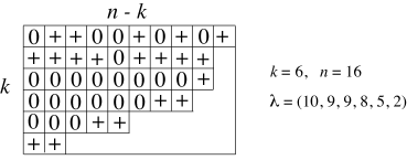
Figure 1: A Le-diagram $(\lambda,D)_{k,n}$.

Theorem 2.8.

[9, Theorem 17.2] Let $S_{\mathcal{M}}^{tnn}$ be a positroid cell in $(Gr_{kn})_{\geq 0}$. For $1\leq r\leq n$, let $I_{r}$ be the index set of the minor in $\mathcal{M}$ which is lexicographically minimal with respect to the order $r<r+1<\dots<n<1<2<\dots r-1$. Then $\mathcal{I}(\mathcal{M}):=(I_{1},\dots,I_{n})$ is a Grassmann necklace of type $(k,n)$.

Lemma 2.9.

[9, Lemma 16.2] Given an irreducible Grassmann necklace $\mathcal{I}$, define a derangement $\pi=\pi(\mathcal{I})$ by requiring that: if $I_{i+1}=(I_{i}\setminus\{i\})\cup\{j\}$ for $j\neq i$, then $\pi(j)=i$. Indices are taken modulo $n$. Then $\mathcal{I}\to\pi(\mathcal{I})$ is a bijection from irreducible Grassmann necklaces $\mathcal{I}=(I_{1},\dots,I_{n})$ of type $(k,n)$ to derangements $\pi(\mathcal{I})\in S_{n}$ with $k$ excedances. The excedances of $\pi(\mathcal{I})$ are in positions $I_{1}$.

Remark 2.10.

If the positroid cell $S_{\mathcal{M}}^{tnn}$ is indexed by the Grassmann necklace $\mathcal{I}$, the derangement $\pi$, and the Γ -diagram $L$, then we also refer to this cell as $S_{\mathcal{I}}^{tnn},S_{\pi}^{tnn}$ and $S_{L}^{tnn}$. The bijections above preserve the indexing of cells, that is, $S_{\mathcal{M}}^{tnn}=S_{{\mathcal{I}}({\mathcal{M}})}^{tnn}=S_{\pi({\mathcal{I}}({\mathcal{M}}))}^{tnn}$.

3 Soliton solutions to the KP equation

Here we explain how to obtain a soliton solution to the KP equation from a point of $(Gr_{kn})_{\geq 0}$.

3.1 From the Grassmannian to the $\tau$-function

We start by fixing real parameters $\kappa_{j}$ such that $\kappa_{1}~{}<~{}\kappa_{2}~{}\cdots~{}<\kappa_{n},$ which are generic, in the sense that the sums $\mathop{\textstyle\sum}\limits_{m=1}^{d}\kappa_{j_{m}}$ are all distinct for $2\leq d\leq k$.

Let $\{E_{j};j=1,\ldots,n\}$ be a set of exponential functions in $(x,y,t)\in\mathbb{R}^{3}$ defined by

$$E_{j}(x,y,t):=\exp\left(\kappa_{j}x+\kappa_{j}^{2}y+\kappa_{j}^{3}t\right).$$

If $E_{i}^{(j)}$ denotes $\partial^{j}E_{i}/\partial x^{j}=\kappa_{i}^{j}E_{i}$, then the Wronskian determinant with respect to $x$ of $E_{1},\dots,E_{n}$ is defined by

$${\rm Wr}(E_{1},\ldots,E_{n})=\det[(E_{i}^{(j-1)})_{1\leq i,j\leq n}]=\prod_{i<j}(\kappa_{j}-\kappa_{i})\,E_{1}\cdots E_{n}.$$

Let $A$ be a full rank $k\times n$ matrix. We define a set of functions $\{f_{1},\ldots,f_{k}\}$ by

$$(f_{1},f_{2},\ldots,f_{k})^{T}=A\cdot(E_{1},E_{2},\ldots,E_{n})^{T},$$

where $(\ldots)^{T}$ denotes the transpose of the vector $(\ldots)$. The $\tau$-function of $A$ is defined by

$$\tau_{A}(x,y,t):={\rm Wr}(f_{1},f_{2},\ldots,f_{k}).$$ (1)

It’s easy to verify that $\tau_{A}$ only depends on which point of $(Gr_{kn})_{\geq 0}$ the matrix $A$ represents.

Applying the Binet-Cauchy identity to the fact that $f_{i}=\mathop{\textstyle\sum}\limits_{j=1}^{n}a_{ij}E_{j}$ for $i=1,\ldots,k$, we get

$$\tau_{A}(x,y,t)=\mathop{\textstyle\sum}\limits_{I\in\binom{[n]}{k}}\Delta_{I}(A)\,E_{I}(x,y,t),$$ (2)

where $E_{I}(x,y,t)$ with $I=\{\kappa_{j_{1}},\ldots,\kappa_{j_{k}}\}$ is defined by

$$E_{I}:={\rm Wr}(E_{j_{1}},E_{j_{2}},\ldots,E_{j_{k}})=\prod_{l<m}(\kappa_{j_{m}}-\kappa_{j_{l}})\,E_{j_{1}}\cdots E_{j_{k}}\,>0.$$

Therefore if $A\in(Gr_{kn})_{\geq 0}$, then $\tau_{A}>0$ for all $(x,y,t)\in\mathbb{R}^{3}$.

Thinking of $\tau_{A}$ as a function of $A$, we note from (2) that the $\tau$ function encodes the information of the Plücker embedding. More specifically, if we identify each function $E_{I}$ with $I=\{j_{1},\ldots,j_{k}\}$ with the wedge product $E_{j_{1}}\wedge\cdots\wedge E_{j_{k}}$, then the map $\tau:Gr_{kn}\hookrightarrow\mathbb{RP}^{\binom{n}{k}-1}$, $A\mapsto\tau_{A}$ has the Plücker coordinates as coefficients.

3.2 From the $\tau$-function to solutions of the KP equation

The KP equation

$$\frac{\partial}{\partial x}\left(-4\frac{\partial u}{\partial t}+6u\frac{\partial u}{\partial x}+\frac{\partial^{3}u}{\partial x^{3}}\right)+3\frac{\partial^{2}u}{\partial y^{2}}=0$$

was proposed by Kadomtsev and Petviashvili in 1970 [1], in order to study the stability of the one-soliton solution of the Korteweg-de Vries (KdV) equation under the influence of weak transverse perturbations. The KP equation also gives an excellent model to describe shallow water waves [11].

It is well known (see e.g. [12]) that the $\tau$-function defined in (1) provides a soliton solution of the KP equation,

$$u_{A}(x,y,t)=2\frac{\partial^{2}}{\partial x^{2}}\ln\tau_{A}(x,y,t).$$ (3)

Note that if $A\in(Gr_{kn})_{\geq 0}$, then $u_{A}(x,y,t)$ is regular.

4 From soliton solutions to soliton graphs

One can visualize such a solution $u_{A}(x,y,t)$ in the $xy$-plane by drawing level sets of the solution for each time $t$. For each $r\in\mathbb{R}$, we denote the corresponding level set by

$$C_{r}(t):=\{(x,y)\in\mathbb{R}^{2}:u_{A}(x,y,t)=r\}.$$

Figure 2 depicts both a three-dimensional image of a solution $u_{A}(x,y,t)$, as well as multiple level sets $C_{r}(0)$. Note that these levels sets are lines parallel to the line of the wave peak.

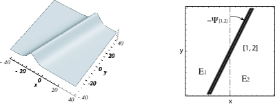
Figure 2: A line-soliton solution from $A=(1,1)\in(Gr_{1,2})_{\geq 0}$. The left figure shows the 3-dimensional profile of $u_{A}(x,y,0)$; the right one shows level sets of $u_{A}(x,y,0)$. $E_{i}$ represents the dominant exponential in the region.

To study the behavior of $u_{A}(x,y,t)$ for $A\in S_{\mathcal{M}}^{tnn}$, we set

$$\hat{f}_{A}(x,y,t) =\underset{J\in\mathcal{M}}{\max}\{\Delta_{J}(A)E_{J}(x,y,t)\}$$

$$=\underset{J\in\mathcal{M}}{\max}\biggl{\{}e^{\ln\bigl{(}\Delta_{J}(A)K_{J}\bigr{)}+\mathop{\textstyle\sum}\limits_{i=1}^{k}(\kappa_{j_{i}}x+\kappa^{2}_{j_{i}}y+\kappa^{3}_{j_{i}}t)}\biggr{\}},$$

where $K_{J}:=\prod_{\ell<m}(\kappa_{j_{m}}-\kappa_{j_{\ell}})>0$. From (2), we see that generically, $\tau_{A}$ can be approximated by $\hat{f}_{A}$.

Let $f_{A}(x,y,t)$ be the closely related function

$${f}_{A}(x,y,t)=\underset{J\in\mathcal{M}}{\max}\left\{\ln\bigl{(}\Delta_{J}(A)K_{J}\bigr{)}+\mathop{\textstyle\sum}\limits_{i=1}^{k}(\kappa_{j_{i}}x+\kappa^{2}_{j_{i}}y+\kappa^{3}_{j_{i}}t)\right\}.$$ (4)

Clearly a given term dominates $f_{A}(x,y,t)$ if and only if its exponentiated version dominates $\hat{f}_{A}(x,y,t)$.

Definition 4.1.

Given a solution $u_{A}(x,y,t)$ of the KP equation as in (3), we define its contour plot $\operatorname{\mathcal{C}}_{t_{0}}(u_{A})$ for each $t=t_{0}$ to be the locus in $\mathbb{R}^{2}$ where $f_{A}(x,y,t=t_{0})$ is not linear.

Remark 4.2.

$\operatorname{\mathcal{C}}_{t_{0}}(u_{A})$ provides an approximation of the location of the wave crests.

It follows from Definition 4.1 that $\operatorname{\mathcal{C}}_{t_{0}}(u_{A})$ is a one-dimensional piecewise linear subset of the $xy$-plane.

Proposition 4.3.

If each $\kappa_{i}$ is an integer, then $\operatorname{\mathcal{C}}_{t_{0}}(u_{A})$ is a tropical curve in $\mathbb{R}^{2}$.

Note that each region of the complement of $\operatorname{\mathcal{C}}_{t_{0}}(u_{A})$ in $\mathbb{R}^{2}$ is a domain of linearity for $f_{A}(x,y,t_{0})$, and hence each region is naturally associated to a dominant exponential $\Delta_{J}(A)E_{J}(x,y,t_{0})$ from the $\tau$-function (2). We call the line segments comprising $\operatorname{\mathcal{C}}_{t_{0}}(u_{A})$ line-solitons. Some of these line-solitons have finite length, while others are unbounded and extend in the $y$ direction to $\pm\infty$. We call these unbounded line-solitons. Note that each line-soliton represents a balance between two dominant exponentials in the $\tau$-function.

Lemma 4.4.

[6, Proposition 5] The dominant exponentials of the $\tau$-function in adjacent regions of the contour plot in the $xy$-plane are of the form $E(i,m_{2},\dots,m_{k})$ and $E(j,m_{2},\dots,m_{k})$.

According to Lemma 4.4, those two exponential terms have $k-1$ common phases, so we call the soliton separating them a line-soliton of type $[i,j]$. Locally we have

$$\tau_{A} \approx\Delta_{I}(A)E_{I}+\Delta_{J}(A)E_{J}$$

$$=\left(\Delta_{I}(A)K_{I}E_{i}+\Delta_{J}(A)K_{J}E_{j}\right)\prod_{l=2}^{k}E_{m_{l}}$$

with $K_{I}=\prod_{j=2}^{k}|\kappa_{i}-\kappa_{m_{j}}|\prod_{l<j}|\kappa_{m_{j}}-\kappa_{m_{l}}|$, so the equation for this line-soliton is

$$x+(\kappa_{i}+\kappa_{j})y+(\kappa_{i}^{2}+\kappa_{i}\kappa_{j}+\kappa_{j}^{2})t=\frac{1}{\kappa_{j}-\kappa_{i}}\ln\frac{\Delta_{I}(A)K_{I}}{\Delta_{J}(A)K_{J}}.$$ (5)

Note that the ratio of the Plücker coordinates labeling the regions separated by the line-soliton determines the location of the line-soliton.

Remark 4.5.

Consider a line-soliton given by (5). Compute the angle $\Psi_{[i,j]}$ between the line-soliton and the positive $y$-axis, measured in the counterclockwise direction, so that the negative $x$-axis has an angle of $\frac{\pi}{2}$ and the positive $x$-axis has an angle of $-\frac{\pi}{2}$. Then $\tan\Psi_{[i,j]}=\kappa_{i}+\kappa_{j}$. Therefore we refer to $\kappa_{i}+\kappa_{j}$ as the slope of the $[i,j]$ line-soliton (see Figure 2).

We will be interested in the combinatorial structure of a contour plot, that is, the pattern of how line-solitons interact with each other. To this end, in Definition 4.7 we will associate a soliton graph to each contour plot.

Generically we expect a point of a contour plot at which several line-solitons meet to have degree $3$; we regard such a point as a trivalent vertex. Three line-solitons meeting at a trivalent vertex exhibit a resonant interaction (this corresponds to the balancing condition for a tropical curve). One may also have two line-solitons which cross over each other, forming an $X$-shape: we call this an $X$-crossing, but do not regard it as a vertex. In general, there exists a phase-shift at each $X$-crossing. However we ignore them in this paper as explained in the footnote 3. Vertices of degree greater than $4$ are also possible.

Definition 4.6.

A contour plot is called generic if all interactions of line-solitons are at trivalent vertices or are $X$-crossings.

The following definition of soliton graph forgets the metric data of the contour plot, but preserves the data of how line-solitons interact and which exponentials are dominant.

Definition 4.7.

Let $\operatorname{\mathcal{C}}_{t_{0}}(u_{A})$ be a generic contour plot with $n$ unbounded line-solitons. Color a trivalent vertex black (respectively, white) if it has a unique edge extending downwards (respectively, upwards) from it. Label each region with the dominant exponential $E_{I}$ and each edge (line-soliton) by the type $[i,j]$ of that line-soliton. Preserve the topology of the metric graph, but forget the metric structure. Embed the resulting graph with bicolored vertices and $X$-crossings into a disk with $n$ boundary vertices, replacing each unbounded line-soliton with an edge that ends at a boundary vertex. We call this labeled graph a soliton graph.

See Figure 3 for an example of a soliton graph. Although we have not labeled all regions or all edges, the remaining labels can be determined using Lemma 4.4.

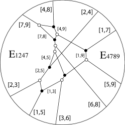
Figure 3: Example of a soliton graph associated to ${\mathcal{S}}_{\pi}^{tnn}$ with $\pi=(7,4,2,8,1,3,9,6,5)$. Each $E_{ijkl}$ represents the dominant exponential in the $\tau$-function. This soliton graph was obtained from a contour plot by embedding it in a disk and coloring vertices appropriately.

5 Permutations and soliton asymptotics

Given a contour plot $\operatorname{\mathcal{C}}_{t_{0}}(u_{A})$ where $A$ belongs to an irreducible positroid cell and $t_{0}$ is arbitrary, we show that the labels of the unbounded solitons allow us to determine which positroid cell $A$ belongs to. Conversely, given $A$ in the irreducible positroid cell $S_{\pi}^{tnn}$, we can predict the asymptotic behavior of the unbounded solitons in $\operatorname{\mathcal{C}}_{t_{0}}(u_{A})$.

Theorem 5.1.

Suppose $A$ is an element of an irreducible positroid cell in $(Gr_{kn})_{\geq 0}$. Consider the contour plot $\operatorname{\mathcal{C}}_{t_{0}}(u_{A})$ for any time $t_{0}$. Then there are $k$ unbounded line-solitons at $y\gg 0$ which are labeled by pairs $[e_{r},j_{r}]$ with $e_{r}<j_{r}$, and there are $n-k$ unbounded line-solitons at $y\ll 0$ which are labeled by pairs $[i_{r},g_{r}]$ with $i_{r}<g_{r}$. We obtain a derangement in $S_{n}$ with $k$ excedances by setting $\pi(e_{r})=j_{r}$ and $\pi(g_{r})=i_{r}$. Moreover, $A$ must be an element of the cell $S_{\pi}^{tnn}$.

The first part of this theorem follows from work of Chakravarty and Kodama [5, Prop. 2.6 and 2.9], [6, Theorem 5]. Our contribution is that the derangement $\pi$ is precisely the derangement labeling the cell $S_{\pi}^{tnn}$ that $A$ belongs to. This fact is the first step towards establishing that various other combinatorial objects in bijection with positroid cells (Grassmann necklaces, plabic graphs) carry useful information about the corresponding soliton solutions.

We now give a concrete algorithm for writing down the asymptotics of the soliton solutions of the KP equation.

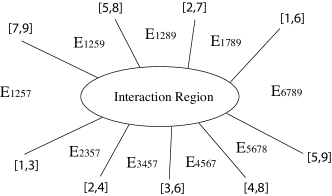
Figure 4: Unbounded line-solitons for $\pi=(6,7,1,2,8,3,9,4,5)$. Each $E_{ijkl}$ shows the dominant exponential in this region.

Theorem 5.2.

Fix generic parameters $\kappa_{1}<\dots<\kappa_{n}$. Let $A$ be an element from an irreducible positroid cell $\operatorname{\mathcal{S}}_{\pi}^{tnn}$ in $(Gr_{kn})_{\geq 0}$. (So $\pi$ must have $k$ excedances.) For any $t_{0}$, the asymptotic behavior of the contour plot $\mathcal{C}_{t_{0}}(u_{A})$ – i.e. its unbounded line-solitons, and the dominant exponentials in its unbounded regions – can be read off from $\pi$ as follows.

• For $y\gg 0$, there is an unbounded line-soliton of type $[i,\pi(i)]$ for each excedance $\pi(i)>i$. From left to right, list these solitons in decreasing order of the quantity $\kappa_{i}+\kappa_{\pi(i)}$.

• For $y\ll 0$, there is an unbounded line-solitons of type $[\pi(j),j]$ for each nonexcedance $\pi(j)<j$. From left to right, list these solitons in increasing order of $\kappa_{j}+\kappa_{\pi(j)}$.

• Label the unbounded region for $x\ll 0$ with the exponential $E_{i_{1},\dots,i_{k}}$, where $i_{1},\dots,i_{k}$ are the excedance positions of $\pi$.

• Use Lemma 4.4 to label the remaining unbounded regions of the contour plot.

Example 5.3.

Consider the positroid cell corresponding to $\pi=(6,7,1,2,8,3,9,4,5)\in S_{9}$. The algorithm of Theorem 5.2 gives rise to the picture in Figure 4. If one reads the dominant exponentials in counterclockwise order, starting from the region at the left, then one recovers the Grassmann necklace $\mathcal{I}$ from Example 2.4. Also note that $\pi(\mathcal{I})=\pi$. See Theorem 6.1.

6 Grassmann necklaces and soliton asymptotics

One particularly nice class of positroid cells is the TP or totally positive Schubert cells. These are the positroid cells indexed by Γ -diagrams which are filled with all $+$’s, or equivalently, the positroid cells indexed by derangements $\pi$ such that $\pi^{-1}$ has at most one descent. When $S_{\pi}^{tnn}$ is a TP Schubert cell, we can make a link between the corresponding soliton solutions of the KP equation and Grassmann necklaces.

Theorem 6.1.

Let $A$ be an element of a TP Schubert cell $\mathcal{S}_{\pi}^{tnn}$, and consider the contour plot $\operatorname{\mathcal{C}}_{t_{0}}(u_{A})$ for an arbitrary time $t_{0}$. Let the index sets of the dominant exponentials of the unbounded regions of $\operatorname{\mathcal{C}}_{t_{0}}(u_{A})$ be denoted $R_{1},\dots,R_{n}$, where $R_{1}$ labels the region at $x\ll 0$, and $R_{2},\dots,R_{n}$ label the regions in the counterclockwise direction from $R_{1}$. Then $(R_{1},\dots,R_{n})$ is a Grassmann necklace $\mathcal{I}$ and $\pi(\mathcal{I})=\pi$.

Theorem 6.1 is illustrated in Example 5.3.

Remark 6.2.

Theorem 6.1 does not hold if we replace “TP Schubert cell” by “positroid cell.”

7 From soliton graphs to generalized plabic graphs

In this section we associate a generalized plabic graph $Pl(C)$ to each soliton graph $C$. We then show that from $Pl(C)$ – whose only labels are on the boundary vertices – we can recover the labels of the line-solitons and dominant exponentials of $C$.

Definition 7.1.

A generalized plabic graph is a connected graph embedded in a disk with $n$ boundary vertices labeled $1,\dots,n$ placed in any order around the boundary of the disk, such that each boundary vertex $i$ is incident to a single edge. Each internal vertex must have degree at least two, and is colored black or white. Edges are allowed to form $X$-crossings (this is not considered to be a vertex).

We now generalize the notion of trip from [9, Section 13].

Definition 7.2.

Given a generalized plabic graph $G$, the trip $T_{i}$ is the directed path which starts at the boundary vertex $i$, and follows the “rules of the road”: it turns right at a black vertex, left at a white vertex, and goes straight through an $X$-crossing. Note that $T_{i}$ will also end at a boundary vertex. The trip permutation $\pi_{G}$ is the permutation such that $\pi_{G}(i)=j$ whenever the trip starting at $i$ ends at $j$.

We use these trips to associate a canonical labeling of edges and regions to each generalized plabic graph.

Definition 7.3.

Given a generalized plabic graph $G$ with $n$ boundary vertices, start at each boundary vertex $i$ and label every edge along trip $T_{i}$ with $i$. Such a trip divides the disk containing $G$ into two parts: the part to the left of $T_{i}$, and the part to the right. Place an $i$ in every region which is to the left of $T_{i}$. After repeating this procedure for each boundary vertex, each edge will be labeled by up to two numbers (between $1$ and $n$), and each region will be labeled by a collection of numbers. Two regions separated by an edge labeled $ij$ will have region labels $S$ and $(S\setminus\{i\})\cup\{j\}$. When an edge is assigned two numbers $i<j$, we write $[i,j]$ on that edge, or $\{i,j\}$ or $\{j,i\}$ if we do not wish to specify the order of $i$ and $j$.

Definition 7.4.

Fix an irreducible cell ${\mathcal{S}}_{\pi}^{tnn}$ of $(Gr_{kn})_{\geq 0}$. To each soliton graph $C$ coming from a point of that cell we associate a generalized plabic graph $Pl(C)$ by:

• labeling the boundary vertex incident to the edge $\{i,\pi_{i}\}$ by $\pi_{i}=\pi(i)$,

• forgetting the labels of all edges and regions.

See Figure 5 for the generalized plabic graph $Pl(C)$ corresponding to the soliton graph $C$ from Figure 3.

Theorem 7.5.

Fix an irreducible cell ${\mathcal{S}}_{\pi}^{tnn}$ of $(Gr_{kn})_{\geq 0}$, and consider a soliton graph $C$ coming from a point of that cell. Then the trip permutation associated to the plabic graph $Pl(C)$ is $\pi$, and by labeling edges and regions of $Pl(C)$ according to Definition 7.3, we will recover the original labels in $C$.

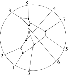
Figure 5: Example of a generalized plabic graph $G(C)$.

We invite the reader to apply Definition 7.3 to Figure 5, and then compare the result to Figure 3.

Remark 7.6.

By Theorem 7.5, we can identify each soliton graph $C$ with its generalized plabic graph $Pl(C)$.

8 Soliton graphs for positroid cells when $t\ll 0$

In this section we give an algorithm for producing a generalized plabic graph $G_{-}(L)$ from the Γ -diagram $L$ of a positroid cell $S_{L}^{tnn}$. It turns out that this generalized plabic graph gives rise to the soliton graph for a generic point of the cell ${\mathcal{S}}_{\begin{sideways}\begin{sideways}$\Gamma$\end{sideways}\end{sideways}}^{tnn}$, at time $t\ll 0$ sufficiently small.

Algorithm 8.1

Given a Γ -diagram $L$, construct $G_{-}(L)$ as follows:

1. Start with a Γ -diagram $L$ contained in a $k\times(n-k)$ rectangle. Label its southeast border by the numbers $1$ to $n$, starting from the northeast corner. Replace $0$’s and $+$’s by “crosses” and “elbows”. From each label $i$ on the southeast border, follow the associated “pipe” northwest, and label its destination by $i$ as well.

2. Add an edge, and one white and one black vertex to each elbow, as shown in the upper right of Figure 6. Forget the labels of the southeast border. If there is an endpoint of a pipe on the east or south border whose pipe starts by going straight, then erase the straight portion preceding the first elbow.

3. Forget any degree $2$ vertices, and forget any edges of the graph which end at the southeast border of the diagram. Denote the resulting graph $G_{-}(L)$.

4. After embedding the graph in a disk with $n$ boundary vertices, we obtain a generalized plabic graph, which we also denote $G_{-}(L)$. If desired, stretch and rotate $G_{-}(L)$ so that the boundary vertices at the west side of the diagram are at the north instead.

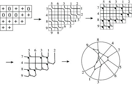
Figure 6: Algorithm 8.1 for ${\mathcal{S}}_{L}^{tnn}$ with $L$ the Le-diagram from the upper left.

Figure 6 illustrates the steps of Algorithm 8.1. Note that this produces the graph from Figure 5.

Theorem 8.2.

Let $L$ be a Γ -diagram and $\pi=\pi(L)$. Then $G_{-}(L)$ has trip permutation $\pi$. Label its edges and regions according to the rules of the road. When $S_{L}^{tnn}$ is a TP Schubert cell, then $G_{-}(L)$ coincides with the soliton graph $G_{t}(u_{A})$, provided that $A\in S_{L}^{tnn}$ is generic and $t\ll 0$ sufficiently small. When $S_{L}^{tnn}$ is an arbitrary positroid cell, we can realize $G_{-}(L)$ as “most” of a soliton graph $G_{t}(u_{A})$ for $A\in S_{L}^{tnn}$ and $t\ll 0$. Moreover, we can construct $G_{t}(u_{A})$ from $G_{-}(L)$ by extending the unbounded edges of $G_{-}(L)$ and introducing $X$-crossings as necessary so as to satisfy the conditions of Theorem 5.2.

9 Reduced plabic graphs and cluster algebras

The most important plabic graphs are those which are reduced [9, Section 12]. Although it is not easy to characterize reduced plabic graphs (they are defined to be plabic graphs whose move-equivalence class contains no graph to which one can apply a reduction), they are important because of their application to cluster algebras and parameterizations of cells.

Theorem 9.1.

Let $A$ be a point of a TP Schubert cell, let $t_{0}$ be an arbitrary time, and suppose that the contour plot $\operatorname{\mathcal{C}}_{t_{0}}(u_{A})$ is generic and has no X-crossings. Then the soliton graph associated to $\operatorname{\mathcal{C}}_{t_{0}}(u_{A})$ is a reduced plabic graph.

Cluster algebras are a class of commutative rings with a remarkable combinatorial structure, which were defined by Fomin and Zelevinsky [13]. Scott [14] proved that Grassmannians have a cluster algebra structure.

Theorem 9.2.

[14] The coordinate ring of the (affine cone over the) Grassmannian has the structure of a cluster algebra. Moreover, the set of labels of the regions of any reduced plabic graph for the TP (totally positive) Grassmannian comprises a cluster for this cluster algebra.

Remark 9.3.

Scott’s strategy in [14] was to show that certain labelings of alternating strand diagrams for the TP Grassmannian gave rise to clusters. However, alternating strand diagrams are in bijection with reduced plabic graphs [9], and under this bijection, Scott’s labelings of alternating strand diagrams correspond to the labelings of regions of plabic graphs induced by the various trips in the plabic graph.

Corollary 9.4.

The Plücker coordinates labeling regions of a generic soliton graph with no X-crossings for $(Gr_{k,n})_{>0}$ form a cluster for the cluster algebra of $Gr_{k,n}$.

Conjecturally, every positroid cell ${\mathcal{S}}_{\pi}^{tnn}$ of the totally non-negative Grassmannian also carries a cluster algebra structure, and the Plücker coordinates labeling the regions of any reduced plabic graph for ${\mathcal{S}}_{\pi}^{tnn}$ should be a cluster for that cluster algebra. In particular, the TP Schubert cells should carry cluster algebra structures. Therefore we conjecture that Corollary 9.4 holds with “TP Schubert cell” replacing “TP Grassmannian.” Finally, there should be a suitable generalization of Corollary 9.4 for arbitrary positroid cells.

10 The inverse problem

The inverse problem for soliton solutions of the KP equation is the following: given a time $t$ together with the contour plot of a soliton solution, can one reconstruct the point of $(Gr_{k,n})_{\geq 0}$ which gave rise to the solution?

Theorem 10.1.

Fix $\kappa_{1}<\dots<\kappa_{n}$ as usual. Consider a generic contour plot of a soliton solution coming from a point $A$ of a positroid cell $S_{\pi}^{tnn}$, for $t\ll 0$. Then from the contour plot together with $t$ we can uniquely reconstruct the point $A$.

The strategy of the proof is as follows. From the contour plot together with $t$, we can reconstruct the value of each of the dominant exponentials (Plücker coordinates) labeling regions of the graph. We have shown how to use the Γ -diagram to construct the soliton graph for a positroid cell when $t\ll 0$ is sufficiently small, which allows us to identify what is the set of Plücker coordinates which label regions of the graph. We then show that this collection of Plücker coordinates contains a subset of Plücker coordinates, which Talaska [15] showed were sufficient for reconstructing the original point of ${\mathcal{S}}_{\pi}^{tnn}$.

Using Theorem 10.1, Corollary 9.4, and the cluster algebra structure for Grassmannians, we can solve the inverse problem for the TP Grassmannian for any time $t$.

Theorem 10.2.

Consider a generic contour plot of a soliton solution coming from a point $A$ of the TP Grassmannian, at an arbitrary time $t$. If the contour plot has no X-crossings, then from the contour plot together with $t$ we can uniquely reconstruct the point $A$.

11 Triangulations of a polygon and soliton graphs

We now explain how to use triangulations of an $n$-gon to produce all soliton graphs for the TP Grassmannian $(Gr_{2,n})_{>0}$.

Algorithm 11.1

Let $T$ be a triangulation of an $n$-gon $P$, whose $n$ vertices are labeled by the numbers $1,2,\dots,n$, in counterclockwise order. Therefore each edge of $P$ and each diagonal of $T$ is specified by a pair of distinct integers between $1$ and $n$. The following procedure yields a labeled graph $\Psi(T)$.

1. Put a black vertex in the interior of each triangle in $T$.

2. Put a white vertex at each of the $n$ vertices of $P$ which is incident to a diagonal of $T$; put a black vertex at the remaining vertices of $P$.

3. Connect each vertex which is inside a triangle of $T$ to the three vertices of that triangle.

4. Erase the edges of $T$, and contract every pair of adjacent vertices which have the same color. This produces a new graph $G$ with $n$ boundary vertices, in bijection with the vertices of the original $n$-gon $P$.

5. Add one unbounded ray to each of the boundary vertices of $G$, so as to produce a new (planar) graph $\Psi(T)$. Note that $\Psi(T)$ divides the plane into regions; the bounded regions correspond to the diagonals of $T$, and the unbounded regions correspond to the edges of $P$.

6. Resolve any non-trivalent vertices into trivalent vertices.

Theorem 11.2.

The graphs $\Psi(T)$ constructed above are soliton graphs for $(Gr_{2,n})_{>0}$. Conversely, any generic soliton graph with no X-crossings for $(Gr_{2,n})_{>0}$ comes from Algorithm 11.1.

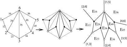
Figure 7: Algorithm 11.1, starting from a triangulation of a hexagon.

Flipping a diagonal in a triangulation corresponds to a mutation in the cluster algebra. In our setting, each mutation may be considered as an evolution along a flow of the KP hierarchy defined by the symmetries of the KP equation.