The First Detection of Blue Straggler Stars in the Milky Way Bulge

Abstract

We report the first detection of Blue Straggler Stars (BSS) in the bulge of the Milky Way galaxy. Proper motions from extensive space-based observations along a single sight-line allow us to separate a sufficiently clean and well-characterized bulge sample that we are able to detect a small population of bulge objects in the region of the color-magnitude diagram commonly occupied young objects and blue strgglers. However, variability measurements of these objects clearly establish that a fraction of them are blue stragglers. Out of the 42 objects found in this region of the color-magnitude diagram, we estimate that at least 18 are genuine BSS. We normalize the BSS population by our estimate of the number of horizontal branch stars in the bulge in order to compare the bulge to other stellar systems. The BSS fraction is clearly discrepant from that found in stellar clusters. The blue straggler population of dwarf spheroidals remains a subject of debate; some authors claim an anticorrelation between the normalised blue straggler fraction and integrated light. If this trend is real, then the bulge may extend it by three orders of magnitude in mass. Conversely, we find that the genuinely young ($<$ 5Gy) population in the bulge, must be at most 3.4% under the most conservative scenario for the BSS population.

1 Introduction

Blue Straggler Stars (hereafter BSS) are thought to be old, hydrogen-burning stars, made hotter and more luminous by accretion and now residing in a region of the color-magnitude diagram (CMD) normally occupied by much younger stars (e.g. Bond & MacConnell, 1971; Livio, 1993; Stryker, 1993). They have been detected in examples of nearly every stellar system - open clusters (e.g. Ahumada & Lapasset, 2007), globular clusters (e.g. Piotto et al., 2004; Lanzoni et al., 2007), dwarf spheroidal (dSph) galaxies (Momany et al., 2007; Mapelli et al., 2007) and the Milky Way stellar halo (Preston & Sneden, 2000; Carney et al., 2001). However, while BSS in the bulge have long been suspected (e.g. Morrison & Harding, 1993), their existence in the bulge as a population has never been proven due to strong contamination from disk stars that fill the same region in the CMD.

By the standards of modern space-baced astrometry, disk and bulge stars have large relative motions ($\sim 5$ mas yr^-1) and thus a reasonably pure sample of bulge stars can be isolated kinematically. Prior use of the Hubble Space Telescope (hereafter HST) to perform this separation indicated that the population of bulge blue stragglers must be small ($\leq$ few percent), but uncertainty in the kinematic contamination (and thus foreground disk objects mimicking BSS), combined with the absence of corroborating evidence like variability, prevented constraint on the BSS population size (Kuijken & Rich, 2002). As a result, BSS have never unambiguously been detected in the Milky Way bulge.

Beyond the intrinsic interest of BSS populations in a predominantly old stellar population, detection of BSS in the Milky Way bulge would be important for galactic structure formation. Most spiral galaxies show flattened “Boxy/Peanut” bulges (see Athanassoula 2005 and Bureau & Athanassoula 2005 for a clear discussion) or a small “Disky bulge” accompanied by ongoing star formation (Kormendy & Kennicutt, 2004). Such a bar-driven arrangement of the stars evolves over a timescale of several Gy, and can be transient with multiple generations of bar (e.g. Combes, 2009). However, chemical evidence suggests the stars themselves mostly formed early and rapidly (e.g. Ballero et al., 2007; McWilliam et al., 2010). While the majority view now is that most stars in the Boxy/Peanut bulge of the Milky Way (which we call here “the bulge”) formed $\sim$10 Gy ago (e.g. Zoccali et al., 2003; Freeman, 2008), the degree to which this star formation was extended over time, is presently only somewhat weakly constrained (Kuijken & Rich, 2002; Zoccali et al., 2008). Thus, better estimates of the young stellar population of the bulge, and thus its evolution, are a natural dividend of constraints on the BSS fraction.

We report our use of a combination of proper motion and variability information to set this constraint. The observations are detailed in Section 2. Section 3 explains the selection of candidate BSS and the analysis used to estimate the size of the true BSS population. Finally in Sections 4 & 5 we discuss the BSS population in the context of stellar populations in general and the formation of the bulge of the Milky Way in particular.

2 Observations

All motions on which we report here were obtained from two-epoch imaging of the SWEEPS (Sagittarius Window Eclipsing Extrasolar Planet Search) field (Sahu et al. 2006) towards the bulge (at $l,b=2.65\arcdeg,-1.25\arcdeg$) using the Wide Field Channel of the Advanced Camera for Surveys on HST, which has pixel scale 49.7 mas pix^-1 (van der Marel et al., 2007). The sight-line passes through the bulge just beneath the galactic mid-plane, passing within $\sim$350pc of the galactic center (but always exterior to the nuclear cluster, which shows ongoing star formation; Launhardt et al. 2002). Full details on the analysis of these extensive HST datasets can be found in Clarkson et al. (2008, hereafter Paper I), Sahu et al. (2006) and Gilliland (2008); we report here the aspects relevant to BSS detection and characterization.

2.1 Astrometry and Photometry

The measurements used are: (i) proper motions down to $F814W=24$ in the SWEEPS field as measured from astrometry in the two epochs; (ii) absolute photometry in $F606W$ & $F814W$, and (iii) time-series photometry of the stars from the continuous seven-day SWEEPS campaign, with gaps only due to Earth occultation.

The techniques used to measure proper motions from the long (339 sec) and short (20 sec) exposures were detailed in Paper I. For objects saturated in the long exposures, motions and errors using the short exposures are substituted. The stellar time-series and absolute photometry were taken from the work of Sahu et al. (2006), in which full details can be found. Difference image analysis techniques (Gilliland, 2008, and references therein) were used to produce the time-series; the noise in the result is very close to Poisson for the majority of objects, and perhaps 30% higher than Poisson for saturated objects. Absolute magnitudes were produced from psf fitting to the image model against which variability was measured (Sahu et al. 2006).

3 Sample selection

The bulge population was extracted using cuts on motion and measurement quality, and the BSS candidates evaluated from this sample (Section 3.1), along with contamination by disk and halo stars that fall into the sample (Section 3.2). Variability information was used to set limits on the size of the young ($\lesssim 5$ Gy) population among bulge BSS candidates (Section 3.3), corrected for periodicity detection incompleteness (Section 3.4). This allowed the size of the true BSS population in the bulge to be bounded (Section 3.5).

3.1 Separation of bulge from field

The streaming of disk stars in front of the bulge in galactic longitude was used to isolate the bulge population. Proper motions were measurable for 188,367 of the 246,793 stars with photometry in the field of view. Stars were selected for further study with proper motion error $\sigma_{l}\leq 0.3$ mas yr^-1 and $\sigma_{b}\leq 0.45$ mas yr^-1, and with crowding parameter $q<0.1$ (see Paper I for definition of the crowding parameter). This latter limit is slightly more restrictive than used in Paper I, and results in a well-measured astrometric sample of 57,384 objects down to $F814W\simeq 23$. Discarding objects saturated in the short exposures then leaves 57,265 well-measured, unsaturated objects. To set the proper motion cut for bulge stars, the distribution of latitudinal proper motion $\mu_{l}$ was measured for stars above the main sequence turn-off (hereafter MSTO), where the disk+BSS and bulge populations trace separate loci in the CMD. Using a proper motion cut $\mu_{l}<-2.0$ mas yr^-1, rejects all but 0.19% of disk stars, while admitting 26% of bulge objects. With error cut at 0.3 mas yr^-1 and $\mu_{l}<-2.0$ mas yr^-1, galactic-longitudinal motions must be detected to at least 6$\sigma$ for inclusion in the cleaned bulge catalogue. Applied to the full error-cleaned sample with astrometry, the motion cut produced a population of 12,762 likely-bulge objects.

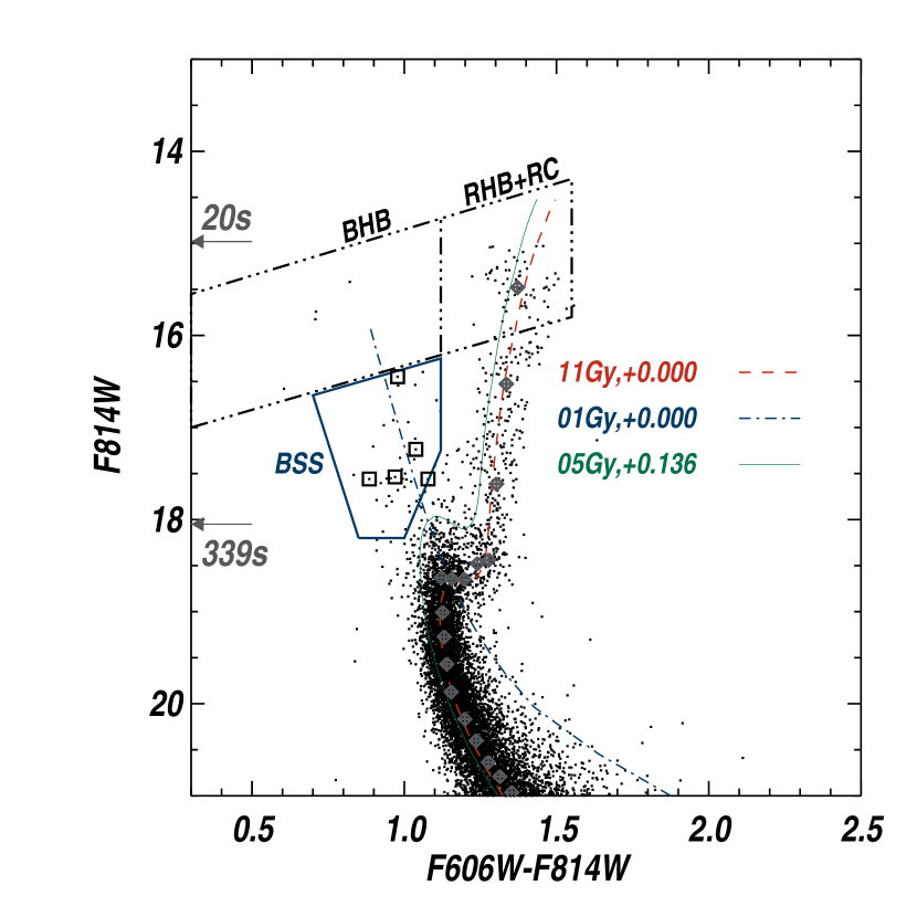
Figure 1: Color-Magnitude Diagram (CMD) of the kinematically selected extreme-bulge population. Isochrones are shown for a young foreground population (blue dash-dot), old bulge population (dashed) and an intermediate-age, slightly metal-poor bulge population (solid). Diamonds show the median bulge population. Ages are indicated, as are the adopted $[Fe/H]$ values. Selection regions for BSS and horizontal branch objects are indicated. Saturation limits in the short and long exposures are marked, and the five BSS candidates exhibiting close binary variable (W UMa) lightcurves are indicated. See Section 3.1.

The BSS selection region was set with the constraints that (i). the bright end should not impinge on the region in which blue horizontal branch objects are expected, and (ii). the faint and red ends should not greatly overlap with the main population of the bulge near the MSTO (see Figure 1 for the selection region adopted in the $F814W$, $F606W-F814W$ CMD). Within this selection-region, 42 objects were found in the kinematically-selected bulge sample.

3.2 Kinematic and photometric contaminants

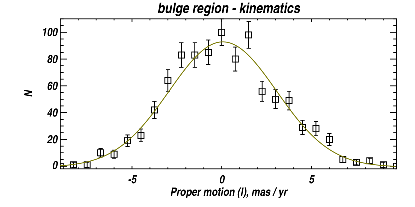
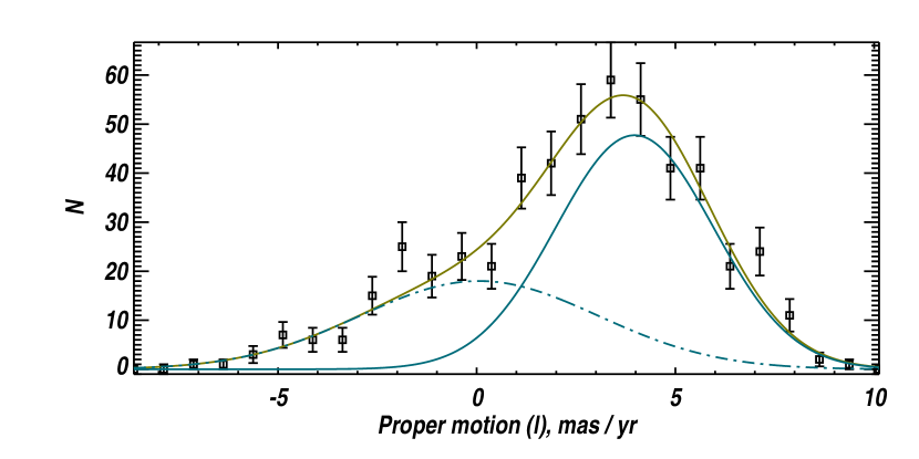
Figure 2: Estimation of the kinematic contamination in the BSS CMD-selection region (Figure 1), due to disk objects. Top: single-component gaussian fit to the distribution of longitudinal proper motion for post-MSTO bulge objects ($\mu_{l,bulge}$), which we use to calibrate the bulge component in the BSS region. Middle: two-component gaussian model fit to the longitudinal proper motion distribution within the BSS region of the CMD ($\mu_{l,BSS}$). Bottom-Left: distribution of recovered number of disk objects in the BSS region under 5,000 Monte Carlo trials. Bottom Right: Distribution of recovered number of disk objects that would pass the kinematic cut $\mu_{l}<-2.0$ mas yr^-1. See Section 3.2.

The number of disk objects amongst our BSS candidate sample was estimated directly from the distribution of longitudinal proper motion $\mu_{l}$. Beginning with the 57,265 objects that are astrometrically well-measured, the longitudinal proper motion distribution is assessed within the post-MSTO bulge sample as shown in Figure 2 (top panel). The CMD selection-region for this post-MSTO bulge sample was constructed by inverting the BSS selection box in color about its reddest point, while keeping the same magnitude range as the BSS sample. We denote the set of longitudinal proper motions of these post-MSTO bulge objects as $\mu_{l,bulge}$. It is clear from Figure 2 that the contribution of any disk objects to this population is very small. This population was fit with a single gaussian component.

The longitudinal proper motion distribution within the BSS selection region we denote by $\mu_{l,BSS}$, and was fit with a model consisting of two gaussian components, one ($\mu_{l,1}$) representing disk objects, one ($\mu_{l,2}$) representing bulge objects (Figure 2, middle panel). The centroid and width of $\mu_{l,2}$ were frozen to the values fit from $\mu_{l,bulge}$; because the BSS and post-MSTO bulge samples cover an identical magnitude range, to first order they should suffer similar instrumental and incompleteness effects. The expected number of disk objects within the BSS selection-box (denoted $N_{d}$) was evaluated from the parameters of the best fit to $\mu_{l,BSS}$ with these constraints (the best-fit to $\mu_{l,BSS}$ shows $\chi^{2}_{\nu}=24.2/26$).

We performed a Monte-Carlo simulation where a large number of proper motion datasets drawn from the best-fit model were generated, and the distribution assessed of recovered values of both the number of disk objects in the BSS region $N_{d}$ and the number that would pass our kinematic cut for bulge objects ($N_{d,<-2.0}$). The results are shown on the bottom panel of Figure 2. The recovered $N_{d,<-2.0}$ is $0.7\pm 0.73$ objects, but the distribution is rather asymmetric - while the most common recovered $N_{d,<-2.0}$ suggests fewer than one contaminant, in some cases up to four contaminants are measured. We therefore adopt 0-4 as the ranges on the contribution from disk objects to our kinematically cleaned bulge sample.

Of the $\sim 6$ estimated halo contaminants (Paper I), of order 0-2 objects would fall into the BSS selection region. So, of 42 objects, we expect $0-6$ objects to have passed our kinematic cuts that do not belong to the bulge.

We investigated by simulation the contamination in our BSS region due to the main bulge population near the MSTO, which might be expected to put outliers in the BSS region. Synthetic bulge populations were constructed with age range $7$-$13$ Gy (Zoccali et al., 2003) and metallicity distribution approximating the bulge (Santiago et al., 2006; Zoccali et al., 2008). Age and metallicity samples were converted to predicted instrumental magnitudes using the isochrones described in Brown et al. (2005). The resulting population was then perturbed by the bulge distance distribution and with a binary population estimated using a variety of binary mass-ratio distributions and binary fractions (Söderhjelm, 2007) to produce simulated bulge-selected populations in the CMD. The resulting number of objects from the main bulge population that happen to fall in the BSS region in the CMD, is $5\pm 2$, over $10^{5}$ trials.

We therefore estimated the total contaminant population at (5-13)/42 objects, leaving (29-37)/42 possible bulge BSS.

3.3 Photometric Variability

BSS may form by a variety of mechanisms (e.g. Abt, 1985; Livio, 1993), including mass transfer in a binary system (McCrea, 1964). This can yield BSS that are presently in binaries (e.g. Andronov et al., 2006; Chen & Han, 2009) with observable radial-velocity periodicities (e.g. Carney et al., 2001; Mathieu & Geller, 2009). For periods $\lesssim$10 days, photometric variations caused by tidal deformation of one or both members may be observed, in the extreme producing a W UMa-type contact binary (Mateo, 1993, 1996).

The variability information from the 2004 epoch (Section 2) allows the tendency for W UMa variability among the BSS candidates to be examined. In a manner similar to Section 3.1, a population composed of mostly disk objects was isolated, this time using longitudinal proper motion $\mu_{l}\geq+3.0$ mas yr^-1 and again requiring 6$\sigma$ motion detection. This test sample indicates the fraction of W UMa-like variables among a young population observed at the same signal to noise range as the bulge objects we wish to probe. Comparison of the W UMa occurrence rate between the mostly-disk and mostly-bulge samples then provides an estimate of the fraction of genuine BSS among the BSS candidates.

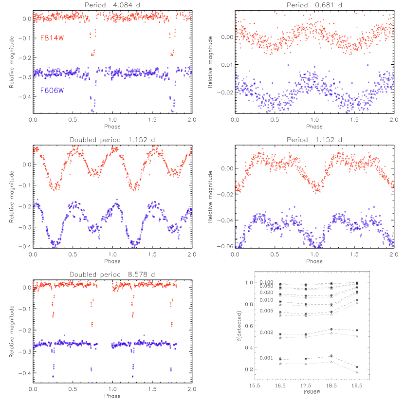
Figure 3: Folded lightcurves for the five objects showing sinusoidal or eclipse-type variability with a period longer than 0.5 days. The object at the top-right is probably a long-period pulsator. The objects at middle-left and bottom-left were detected at half the likely true period, as suggested by differing eclipse depths half a period apart. Bottom Right: Completeness to W UMa variability from the HST dataset. Left: fraction of injected W UMa lightcurves recovered as a function of magnitude and amplitude. Injected variation amplitudes $\Delta V/V$ are labeled next to each set of curves. For each set of curves, from top to bottom, symbols represent periods 0.4, 0.8, 1.7, 3.4 and 7.0d respectively; in practice, all the limits for a given amplitude overlap except for the 7d set.

To avoid confusion with pulsators, systems were not counted among the W UMa if the dominant period detected $P$ was shorter than $0.5$d, or if significant phase or frequency variation was present along the observation interval (Gilliland, 2008). Note that we do not eliminate possible pulsators from our BSS candidate table, as BSS can also show photometric pulsations (Mateo, 1993). Each variable lightcurve was visually examined to determine if its morphology resembles that of W Uma objects or close eclipsing binaries found in other systems (e.g. Mateo, 1993; Albrow et al., 2001). W UMa’s were much more populous amongst the bulge-selected population: of the 42 bulge-selected objects, four show W UMa-type variability (one additional object is apparently a long-period pulsator; Figure 3). Of this four, one object only has a single eclipse event recorded and awaits confirmation. Conversely, none of the 81 disk-selected objects show W UMa photometric variability.

3.4 Periodicity completeness correction

The completeness of the Lomb-Scargle (hereafter LS) variability search to W UMa variables was estimated through simulation. Real lightcurves with no significant periodicity detection (peak LS power $<$5) were injected with W UMa-type lightcurves (following the description of Rucinski, 1993) under a log-uniform period distribution. Synthetic W UMa systems were denoted “detected” if the peak in the Lomb-Scargle periodogram was within 10% of the input period, the signal was present in the lightcurves in both filters, and showed LS peak power greater than 13 (the 99% significance level, defined as the peak LS power exceeding that returned by 99% of trials with no periodicity injected). The process was repeated for input variation amplitudes $\Delta$mag/mag = 0.1, 0.05, 0.02, 0.01, 0.005, 0.002, 0.001 and period bins 0.4, 0.8, 1.7, 3.4 and 7.0d (Figure 3). The dependence of the detection completeness on injected period is rather weak but the dependence on amplitude is clear; at least $88\%$ of systems with 2% fractional amplitude variation were detected, and 70% at the 0.5% amplitude level.

To map signal amplitude to system inclinations, synthetic W UMa lightcurves were simulated using the Wilson & Devinney (1971) code as implemented in the Nightfall package indicating that at most $\sim$70% of W UMa type systems would be detectable down to binary inclination $\sim$45$\arcdeg$, so we are sensitive to perhaps 35% of the true W UMa population. This implies that the 3-4 detected W UMa trace an underlying population of 9-11 systems with W UMa-like system parameters, so at least $9$-$11$ of the 42 BSS candidate objects have W UMa system parameters, and are therefore not young.

If, as our measurements suggest, 9-11 of the 42 BSS candidates are present-day W UMa objects, we can ask what fraction of the BSS candidates are in binaries of any orbital period. The period distribution for bulge BSS presently in binaries is unknown; we use observations of the solar neighbourhood and open clusters as proxies for the bulge population.

Carney et al. (2001) report spectroscopic periods for 6/10 high-proper motion blue metal-poor (hereafter BMP) stars in the solar neighborhood, isolating BSS candidates by virtue of de-reddened colors bluer than the MSTO of globular clusters of comparable metallicity (Carney et al., 1994). That study also reports a re-analysis of the radial velocities of the BMP sample of Preston & Sneden (2000), finding ten spectroscopic BMP orbits for a grand total of sixteen spectroscopic orbits among 6 BSS candidates and 10 further BMP that may be BSS. This yields 2/16 objects with $\log_{10}(P_{orb})<1$ and 14/16 with $1.0\leq\log_{10}(P)<3.2$ (with one possible very long-period binary not included in this sample). Thus, in the solar neighborhood perhaps 1/8 of the total binary BSS population resides in short-period binaries, with $\log_{10}(P_{orb})<1.0$.

Turning to the open clusters, Mathieu & Geller (2009) find a high binary fraction and broadly similar period distribution amongst BSS candidates in the $\sim 7$ Gy-old open cluster NGC 188. There, 16/21 BSS candidates are in binaries. Of these sixteen objects, two show $\log_{10}(P)<1.0$ while the remaining 14 all show $1.0\leq\log_{10}(P)<3.5$. For the $\sim 5$ Gy-old open cluster NGC 2682 (M67), Latham (2007) reports two BSS in binaries with $\log_{10}(P_{orb}<1)$ and five with $1.0\leq\log_{10}(P_{orb})<3.1$ (Figure 3 of Perets & Fabrycky, 2009). Thus, in open clusters the short-period binaries may make up between about 1/8 and 2/7 of the total population of BSS in binaries.

The period distribution for main-sequence binaries of several types is collated in Kroupa (1995). For $P_{orb}\lesssim 3.5$ the number of binaries increases with $P_{orb}$ at least as steeply as a log-uniform distribution (Kroupa, 1995). If BSS in binaries in the bulge follow a similar distribution, then binary BSS with $\log_{10}(P)<1$ would make up at most about 1/3 of the total population with $\log_{10}(P)<3.0$.

Taken together, these estimates suggest that, if all the W UMa are indeed BSS presently in binaries, then BSS in binaries could by themselves account for all the 29-37 non-contaminant objects among our candidate BSS.

3.5 Bounds on the true BSS population in the bulge

As none of the kinematically-selected disk objects show W UMa characteristics, the W UMa stars in the BSS region are unlikely to be disk stars. Furthermore, W UMa variability is expected to be a natural evolutionary state of some of the blue stragglers. Thus, the detection of W UMa variability in the BSS region of the bulge CMD certifies these stars as true bulge blue stragglers. Hence, we conclude that the $9-11$ W UMa objects are in fact bulge BSS, from a possible bulge BSS population of $29$-$37$ (Section 3.2). This leaves $18$-$28$ bulge objects whose nature remains undetermined. It is unlikely that W UMa variables make up the entire BSS population in the bulge. Based on arguments in Section 3.4, we consider the BSS population with binary periods $\log_{10}(P)<1$ to comprise at most half of the population of BSS with any orbital period. We therefore consider two extreme scenarios: 1. Optimistic: all of the remainder are bulge BSS – thus there are no genuinely young bulge objects in our sample, leaving $29-37$ BSS, and 2. Conservative: our W UMa objects make up half of the BSS among our sample, suggesting 18-22 genuine BSS and $7-19$ possibly young bulge objects.

In addition, a significant fraction of the bulge BSS population may exist with no binary companion or in very wide binaries, as indicated by population studies (e.g. Andronov et al., 2006; Chen & Han, 2009) and observations of clusters and the solar neighbourhood (e.g. Ferraro et al., 2006; Carney et al., 2001). Therefore the true BSS population in the bulge probably lies between the “conservative” and “optimistic” scenarios outlined above.

4 Discussion

4.1 Normalization of $N_{BSS}$

As probes of binary evolution, BSS indirectly probe the star formation history of stellar populations in their own right. To compare the bulge BSS population with that of other stellar systems, we normalize by the number of horizontal branch objects in the system; $S_{BSS}=N_{BSS}/N_{HB}$. We adopt $N_{HB}=N_{BHB}+N_{RHB}+N_{RC}$, where the three terms denote the Blue and Red horizontal branch stars, and the Red Clump stars respectively, and thus cover the full metallicity range of post-MS core He-burning objects. This is the convention used for the dwarf spheroidals (e.g. Carrera et al., 2002; Mapelli et al., 2007; Momany et al., 2007, although some authors choose not to include $N_{RC}$ explicitly if none are found in their sample); open clusters (de Marchi et al., 2006) and the globular clusters (Piotto et al., 2004, though here the definition of $N_{HB}$ is not explicitly stated). The exception is the stellar halo, where $N_{HB}=N_{BHB}$ is adopted because only BHB can be distinguished kinematically and photometrically from the local disk population (Preston et al., 1991).

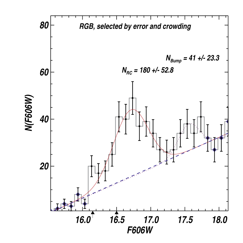
Figure 4: Estimation of the red clump population $N_{RC}$ for the bulge. We use the sample selected for astrometric error and crowding, and use the population within the bulge RGB rather than cutting by proper motion to afford sufficient statistics to constrain $N_{RC}$ accurately. Diamonds show bins selected for the fit to the underlying RGB population (dashed line), subtracted before estimating $N_{RC}$. The fits to the RC population (solid line) and RGB bump (dotted line) are indicated, as are the population sizes in the RC and RGB bump (the latter is marginally detected). Triangles indicate astrometric saturation limits for the $RC$ at the blue and red ends of the selection box (Figure 1). See Section 4.1

The kinematic cuts leave too sparse a population to accurately disentangle the RC from the underlying Red Giant Branch (RGB). We therefore estimate $N_{RC}$ from the $F606W$ histogram along the RGB only after selection by astrometric error and crowding parameter, and scale the result to the bulge population passing the full set of cuts (Section 3.1). Figure 4 shows the selection; the marginally-detected RGB Bump (hereafter RGBB) is masked out as well as the RC before fitting the continuum due to the RGB; Gaussian components fit to the RC and RGBB then yield the number of objects in each population over the RGB continuum. Bootstrap monte carlo sampling before producing the histogram is used to estimate the fitting uncertainty for a given binning scheme. We find $N_{RC}=180\pm 53$ while the RGBB is detected at more marginal significance; $N_{RGBB}=41\pm 23$. Our estimate of $N_{RC}=180\pm 53$ scales to the 26% of bulge objects surviving the full kinematic cuts, as $47\pm 14$ objects. Even in the short exposures, roughly 15% of this population would saturate and thus not enter the bulge sample (Figure 4), so that we would expect $40\pm 12$ RC objects to fall within the bulge sample. This figure includes the RHB objects.

The contribution from BHB is difficult to estimate for the bulge, but is clearly rather small - it vanishes against the much larger foreground disk population without kinematic selection. Unlike the RC+RHB selection region, saturation of the astrometric exposures is not an issue for the BHB selection region we adopt (Figure 1). Altogether, four objects are found in the BHB + RHB selection region; of order one object may be a kinematic contaminant. We therefore consider $(3-4\pm 1\sigma_{\rm Poisson})=2-6$ as the limits on $N_{BHB}$.

Thus we estimate the total $N_{HB}=$30-58 objects among the same sample from which the BSS were estimated. Our estimate of $18\leq N_{BSS}\leq 37$, then leads to $0.31\leq(S_{BSS}=N_{BSS}/N_{HB})\leq 1.23$.

4.2 Comparison to other systems

For the halo, Preston & Sneden (2000) estimate $N_{BSS}/N_{BHB}=5$, though their selection criteria appear to admit a population that is a factor 2 lower; we adopt $2.5\leq S_{BSS}\leq 5$ for the halo. The upper limit $N_{BHB}=6$ for the bulge indicates the lower limit $N_{BSS}/N_{BHB}\geq 3.0$. Thus our BSS fraction is marginally consistent with that of the halo, but as yet the statistics are too poor to support further interpretation.

In principle it would be of interest to compare the normalised blue straggler population in the bulge with those from the dSph and the clusters. In particular, the collection of $S_{BSS}$ vs integrated light $M_{V}$ (a proxy for the mass) for clusters and dSph of Momany et al. (2007) suggests differing trends for clusters and spheroidals, against which the bulge would make an interesting comparison.

In practice, however, the true variation of blue straggler population with mass, is still far from settled observationally; we use the case of the dSph objects Draco and Ursa Minor as a case study. For these objects, different authors reach strikingly different conclusions using data from the same facility (the Wide Field Camera on the 2.5m Isaac Newton Telescope). In their compilation, Momany et al. (2007) quote $S_{BSS}\approx 1.23,1.35$ for Draco (Carrera et al., 2002) and Ursa Minor (Aparicio et al., 2001) respectively, while Mapelli et al. (2007) obtain instead $S_{BSS}\approx 0.25,0.3$ respectively for the same systems. (Both studies conclude that Draco and Ursa Minor are true fossil systems, with no extensive present-day star formation activity.)

The two studies differ in the choice of selection region for BSS on the CMD; that of Mapelli et al. (2007) is about a factor two smaller than that of Momany et al. (2007, and refs therein), and is separated from the MSTO by a larger distance in the CMD. Thus it is unsurprising that the more conservative BSS region produces a lower number of BSS candidates; our problem is choosing the study most appropriate for comparison to our own work. The BSS selection region we have adopted is most similar to that of Momany et al. (2007, compare our Figure 1 with Figure 1 of that paper), and is consistent with the selection regions used for the cluster studies cited therein. Our belief is therefore that Momany et al. (2007) is the most appropriate for comparison to our own estimate.

In addition to photometric selection effects, the sample of objects under consideration includes systems of differing turn-off mass, which means the BSS populations uncovered in these systems may have quite different formation mechanisms from each other. Furthermore, our sample of BSS candidates is different from those of the external systems since our candidates were found in a pencil-beam survey through a narrow part of the bulge. A better interpretation requires population synthesis modeling, which is beyond the scope of the present investigation. With these caveats in mind, we present the BSS fraction of the bulge compared to the Momany et al. (2007) selection in the hope that it will provoke just such an investigation.

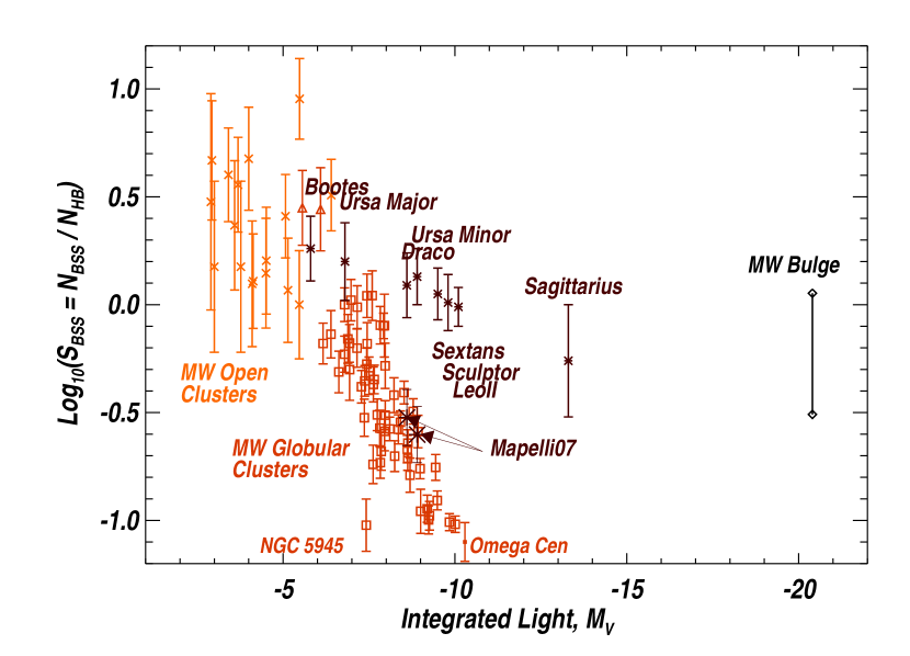
Figure 5: Comparison of the normalized bulge blue straggler fraction $S_{BSS}$ (limits: black diamonds) with other stellar populations, as a function of integrated light $M_{V}$. These are: dwarf spheroidal galaxies without prominent current star formation (asterisks; each is labeled), Milky Way globular clusters (boxes), the Milky Way globular clusters NGC 6717 and NGC 6838, which may have significant field-star contamination (triangles) and the Milky Way open clusters (crosses). Literature points are from the compilation of Momany et al. (2007 and refs therein) except for the bulge (this work), and the redeterminations of the BSS fraction in Draco and Ursa Major by Mapelli et al. (2007; indicated with arrows as they overlap the cluster sequence). See Section 4.2

We use COBE photometry to estimate $M_{V}\sim 20.4$ for the bulge (Dwek et al., 1995). When placed on the $S_{BSS}/M_{V}$ diagram, the bulge appears to be consistent with the trend pointed out by Momany et al. (2007). If the ($M_{v},S_{BSS}$) trend reported in Momany et al. (2007) is indeed borne out by further observation, then the bulge may extend this trend by over seven magnitudes in $M_{V}$ (or, assuming constant M/L ratio, nearly three orders of magnitude in mass; Figure 5). What this suggests about BSS evolution in the bulge as compared to the dwarf spheroidals, is unclear at present, and we defer interpretation until the Momany et al. (2007) trend has been further established or falsified. It should also be borne in mind that our study samples the bulge quite differently (narrow and deep) to the dSph galaxies (wide-area but relatively shallow); however as ours is the first study to provide a measurement of $S_{BSS}$ for the bulge, we show its location on the $S_{BSS}$-$M_{V}$ diagram to stimulate further investigation.

We can say that the bulge is discrepant from the sequence suggested by the globular clusters; for it to lie on the cluster trend we would have to have observed no BSS in our sample at all.

4.3 Young-bulge population

For the purposes of this report we define “young objects” as stars already on the main sequence, with ages $\lesssim 5$ Gy. Our photometry covers main sequence objects up to about two solar masses, so the main sequence lifetime of all objects in our sample is long compared to the time spent on the Hyashi track.

The simplest estimate assumes that the fractional contribution by young objects is the same across all luminosity bins. In this case the young-bulge population is estimated from the number of non-BSS bulge objects in the BSS region of the CMD (0-19; Section 3.5) and the total number of bulge objects in the same magnitude range and with the same kinematic and error selection (346 objects). This yields a young-bulge fraction in this luminosity strip, of 0-5.5%.

A more complete estimate extrapolates the young population within the BSS selection-box to the entire bulge sample for which we have astrometry. This extrapolation is complicated by differing incompleteness to astrometry above and below the MSTO (Section 2), and by our lack of knowledge of the luminosity function of young bulge objects.

To estimate this scaling, we make two assumptions: (i). that the young bulge population and disk population both follow the same Salpeter mass function (i.e. $dN/dm\propto m^{-2.35}$) and the same mass-magnitude relationship, and (ii). that the astrometric selection effects for disk and young bulge objects vary with instrumental magnitude in the same way. The second assumption allows us to account for astrometric incompleteness in the young-bulge objects, while the first allows us to correct the estimate for the fact that the disk and bulge populations are seen at different distance moduli and thus sample different parts of the mass function.

Denoting the number of objects within the BSS selection region as $N_{BSS}$ and the number from the base of the BSS region in the CMD to the faint limit of our kinematically-cleaned sample ($F814W=23$) as $N_{faint}$ we expect

$$\left(\frac{N_{faint}}{N_{BSS}}\right)_{disk} = \left(\frac{c_{faint}}{c_{BSS}}\right)_{disk}\left(\frac{n_{faint}}{n_{BSS}}\right)_{disk}$$

$$\left(\frac{N_{faint}}{N_{BSS}}\right)_{young~{}bulge} = \left(\frac{c_{faint}}{c_{BSS}}\right)_{young~{}bulge}\left(\frac{n_{faint}}{n_{BSS}}\right)_{young~{}bulge}$$ (1)

where the quantities $c_{BSS}$ and $n_{BSS}$ refer to the astrometric completeness and the integral of the mass function respectively within the magnitude limits of the BSS selection box. We do not distinguish between the initial and present-day mass function for the disk and young bulge populations.

Under our assumption (ii) above that $\left(\frac{c_{faint}}{c_{BSS}}\right)_{disk}=\left(\frac{c_{faint}}{c_{BSS}}\right)_{young~{}bulge}$, estimates of $\left(\frac{n_{faint}}{n_{BSS}}\right)_{disk}$, $\left(\frac{n_{faint}}{n_{BSS}}\right)_{young~{}bulge}$ and $\left(\frac{N_{faint}}{N_{BSS}}\right)_{disk}$ allow us to solve for $\left(\frac{N_{faint}}{N_{BSS}}\right)_{young~{}bulge}$. The first two quantities may be estimated from the mass function under assumption (i) above, while the third can be estimated from our kinematic dataset.

We use the zero-age, solar metallicity disk isochrone of Sahu et al. (2006) to convert magnitude limits to mass limits for both the disk and young-bulge populations. Investigation of a wider range of metallicities for young objects is beyond the scope of this report. In reality, the disk stars are distributed over a range of distances along the line of sight, although as the largest contribution of disk stars comes from the Sagittarius spiral arm we restrict ourselves here to a single distance for the disk population. The isochrone allows us to convert magnitude limits in the “BSS” and “faint” samples to mass limits for the disk population in order to estimate $\left(\frac{n_{faint}}{n_{BSS}}\right)_{disk}\equiv f_{MF,disk}$. To estimate this quantity for the young bulge population, the difference in distance moduli for bulge and disk are used to estimate the corresponding mass limits for the young-bulge sample. Table 2 shows the mass limits adopted and the correction factors adopted from this analysis.

All that remains is to estimate $\left(\frac{N_{faint}}{N_{BSS}}\right)_{disk}$ from observation. We follow a similar method to the fitting of the size of the bulge and disk population within the BSS region as described in Section 3.2 above; the longitudinal proper motion distribution $\mu_{l}$ is estimated for a series of magnitude strips beneath the MSTO and the number of disk objects in each magnitude bin is estimated from the component of the fit that corresponds to the disk population. The results are in Figure 6; the number of disk objects in the BSS region is $N_{d,BSS}=354\pm 23$ while the number below the BSS region is $N_{d,faint}=8781\pm 617$ objects, resulting in the scaling $\left(\frac{N_{faint}}{N_{BSS}}\right)_{disk}=24.8\pm 2.4$. This then means $\left(\frac{N_{faint}}{N_{BSS}}\right)_{young~{}bulge}=(24.8\pm 2.4)\times\left(\frac{5.20}{5.84}\right)=22.0\pm 2.1$. We remind the reader that we are concerned in this section entirely with the young bulge objects.

This means that under our “conservative” scenario, the 7-19 young bulge objects suggested by our dataset within the BSS region would scale to approximately 163-437 young bulge objects across the entire magnitude range. As a fraction of the 12,762 kinematically-selected bulge objects, this young population would make up as much as $1.3\%-3.4\%$ of the bulge population, under our “conservative” scenario for the number of true BSS in the bulge.

The small young-bulge population is difficult to reconcile with the recent discovery of a metallicity transition (high to low moving outward from the galactic center) that has been reported at $\sim$0.6-1kpc beneath the mid-plane (Zoccali et al., 2008). If this transition really does indicate a more metal-rich population interior to 0.6kpc, then the lack of young bulge objects along our sight line would suggest that this metal-rich interior population is not a younger population. Corroborating this suggestion, Ortolani et al. (1995) considered the age of the bulge in Baade’s Window and found it similar to that of the globular clusters.

In addition, a growing number of main sequence objects in the bulge are becoming spectroscopically accessible by microlensing; at present fifteen bulge dwarfs have been spectroscopically studied in a box $10\arcdeg\times 8\arcdeg$ about the galactic center (Bensby et al., 2010). Among these objects, three are spectroscopically dated to $\lesssim 5$ Gy, far more than the $<3\%$ we would predict. If we have somehow vastly underestimated our kinematic contamination from the disk, the discrepancy is only sharpened because the true sample of young bulge objects would then be reduced still further. At least part of this discrepancy may be due to the fact that most of the lensed sources are not in the inner bulge region that we probe here. In addition, star formation rates within the bulge probably do vary strongly over the large spatial scales probed by microlensing studies (e.g. Davies et al., 2009). We note that all three young objects in the Bensby et al. (2010) sample (their objects 310, 311 and 099) are degrees away from our field on the plane of the sky, at negative galactic longitudes. We await further results on the spatial distribution of metallicity and age within the bulge, with great interest.

5 Conclusions

HST observations of a low-reddening window through the bulge have yielded the first detection of Blue Straggler Stars (BSS) in the bulge of the Milky Way. By combining kinematic discrimination of bulge/disk objects with variability information afforded by an $HST$ dataset of unprecedented length (from space and for the bulge), we find that:

$\bullet$ Of the 42 BSS candidates identified with the bulge, between 18-37 are true BSS. We estimate for the horizontal branch $N_{HB}=30$-$58$ with the same kinematic selection, suggesting $0.31\leq N_{BSS}/N_{HB}\leq 1.23$.
$\bullet$ If the trend in normalized BSS fraction against integrated light suggested by Momany et al. (2007) is real, the bulge may extend this trend by nearly three orders of magnitude in mass.
$\bullet$ Normalized appropriately, the BSS population in the bulge is marginally consistent with that in the inner halo but the allowed range for the bulge is very broad.
$\bullet$ The truly-young ($\lesssim 5$Gy) stellar population of the bulge is at most 3.4%, but could be as low as 0 along our sight-line.
$\bullet$ If the recently-discovered metallicity transition $\sim 0.6-1$kpc beneath the mid-plane (Zoccali et al., 2008) does indeed indicate a population transition, then the more metal-rich population does not have a significant component of age $\lesssim 5$ Gy.

In the old metal rich Galactic bulge, we may therefore conclude that blue stragglers are a small component of the stellar population (18-37 of 12,762 kinematically selected bulge objects), and would not significantly affect the integrated light of similar unresolved populations.

6 Acknowledgments

Based on data taken with the NASA/ESA Hubble Space Telescope obtained at the Space Telescope Science Institute (STScI). Partial support for this research was provided by NASA through grants GO-9750 and GO-10466 from STScI, which is operated by the Association of Universities for Research in Astronomy (AURA), inc., under NASA contract NAS5-26555. RMR acknowledges financial support from AST-0709479 and also from GO-9750. MZ and DM are supported by the FONDAP Center for Astrophysics 15010003, the BASAL CATA Center for Astrophysics and Associated Technologies PFB-06, the MILENIO Milky Way Millennium Nucleus, P07-021F, and FONDECYT 1110393 and 1090213.

We thank Yazan al-Momany for kindly providing the cluster and dwarf spheroidal blue straggler populations in electronic form. WIC thanks Hans-Walter Rix, George Preston, Con Deliyannis and Christian Howard for useful discussion, and the astronomy department at Indiana University, Bloomington, for hospitality during early portions of this work. We thank Ron Gilliland for his dedication of time and effort to the production of the lightcurves on which this work is partly based. Finally, we thank the anonymous referee, whose comments greatly improved the presentation of this work.

Facilities: HST (ACS).

Figure 6: Estimating the scaling of the number of young objects within the BSS selection region (Figure 1) to the full kinematic sample, in the presence of datasets of differing depth. For each magnitude strip, the marginal $\mu_{l}$ distribution is fit by a two-component gaussian, identified with the disk and bulge. The fractional contribution from the disk is then identified from the fits, and the errors estimated by Monte Carlo (Section 3.2). Top: disk fraction among the magnitude strips below the BSS CMD region; the brightest bin contains the MSTO itself. Bottom: histogram of the number of disk objects detected in the sample, this time with the number of disk objects detected in the BSS region included (brightest bin). See Section 4.3.

Table 1: Table of Bulge Blue Straggler Candidates.

f814W	f606W	RA (J2000.0)	Dec (J2000.0)	P(d)
16.397	17.458	17h 58m 55.441s	-29$\arcdeg$ 11′ 1.110′′	-
16.448	17.426	17h 59m 1.516s	-29$\arcdeg$ 10′ 49.401′′	1.152
16.537	17.573	17h 58m 58.208s	-29$\arcdeg$ 12′ 1.974′′	-
16.544	17.524	17h 59m 7.983s	-29$\arcdeg$ 11′ 8.239′′	-
16.705	17.811	17h 59m 5.742s	-29$\arcdeg$ 12′ 3.695′′	-
16.822	17.941	17h 59m 2.823s	-29$\arcdeg$ 10′ 18.616′′	-
16.921	17.885	17h 59m 6.525s	-29$\arcdeg$ 13′ 25.552′′	-
16.942	17.955	17h 58m 59.127s	-29$\arcdeg$ 12′ 56.727′′	-
16.975	17.908	17h 59m 1.232s	-29$\arcdeg$ 11′ 14.057′′	-
17.121	18.157	17h 59m 1.975s	-29$\arcdeg$ 11′ 44.373′′	-
17.175	18.111	17h 59m 7.283s	-29$\arcdeg$ 12′ 56.907′′	-
17.207	18.105	17h 58m 57.713s	-29$\arcdeg$ 12′ 0.897′′	-
17.237	18.275	17h 59m 4.579s	-29$\arcdeg$ 11′ 1.411′′	8.578
17.330	18.316	17h 59m 6.396s	-29$\arcdeg$ 10′ 23.907′′	-
17.345	18.378	17h 59m 2.214s	-29$\arcdeg$ 10′ 45.657′′	-
17.454	18.446	17h 59m 4.413s	-29$\arcdeg$ 10′ 28.276′′	-
17.500	18.503	17h 58m 55.138s	-29$\arcdeg$ 13′ 4.462′′	-
17.512	18.598	17h 59m 7.624s	-29$\arcdeg$ 10′ 32.762′′	-
17.515	18.349	17h 58m 58.896s	-29$\arcdeg$ 13′ 15.047′′	-
17.537	18.507	17h 59m 1.420s	-29$\arcdeg$ 12′ 21.630′′	1.152
17.552	18.507	17h 58m 53.865s	-29$\arcdeg$ 10′ 32.655′′	-
17.554	18.496	17h 58m 54.981s	-29$\arcdeg$ 11′ 18.907′′	-
17.557	18.552	17h 59m 3.068s	-29$\arcdeg$ 12′ 52.866′′	-
17.559	18.444	17h 59m 5.433s	-29$\arcdeg$ 12′ 10.876′′	0.681
17.559	18.637	17h 58m 56.862s	-29$\arcdeg$ 11′ 8.062′′	4.084
17.564	18.571	17h 58m 53.759s	-29$\arcdeg$ 13′ 7.067′′	-
17.586	18.609	17h 59m 8.024s	-29$\arcdeg$ 11′ 35.341′′	-
17.604	18.527	17h 59m 6.340s	-29$\arcdeg$ 11′ 16.109′′	-
17.646	18.647	17h 59m 4.582s	-29$\arcdeg$ 11′ 46.148′′	-
17.680	18.659	17h 58m 55.199s	-29$\arcdeg$ 11′ 22.063′′	-
17.744	18.694	17h 58m 58.157s	-29$\arcdeg$ 10′ 54.293′′	-
17.783	18.833	17h 58m 59.460s	-29$\arcdeg$ 10′ 37.722′′	-
17.788	18.697	17h 59m 2.043s	-29$\arcdeg$ 10′ 19.798′′	-
17.799	18.839	17h 59m 0.994s	-29$\arcdeg$ 12′ 2.624′′	-
17.805	18.764	17h 59m 7.892s	-29$\arcdeg$ 10′ 50.466′′	-
17.853	18.794	17h 59m 6.990s	-29$\arcdeg$ 10′ 28.606′′	-
17.853	18.868	17h 58m 56.398s	-29$\arcdeg$ 12′ 16.750′′	-
17.865	18.906	17h 59m 3.512s	-29$\arcdeg$ 13′ 22.640′′	-
17.877	18.915	17h 59m 2.502s	-29$\arcdeg$ 13′ 26.309′′	-
17.915	18.933	17h 58m 53.989s	-29$\arcdeg$ 10′ 26.682′′	-
18.106	19.110	17h 59m 6.057s	-29$\arcdeg$ 11′ 18.876′′	-
18.131	19.061	17h 58m 55.690s	-29$\arcdeg$ 12′ 34.222′′	-

	Mass limits - BSS region	Mass limits - “Faint” region	$\left(\frac{n_{faint}}{n_{BSS}}\right)_{disk}\equiv f_{MF}$
	$(16.2\leq F814W<18.2)$	$(18.2\leq F814W<23.0)$
Disk	$1.12\leq\frac{M}{M_{\odot}}<1.68$	$0.43\leq\frac{M}{M_{\odot}}<1.12$	$f_{MF,disk}=5.84$
Bulge	$1.41\leq\frac{M}{M_{\odot}}<2.11$	$0.53\leq\frac{M}{M_{\odot}}<1.41$	$f_{MF,bulge}=5.20$

Table 2: Mass-function correction used when scaling the number of objects within the BSS selection region to the full magnitude range $(16.2\leq F814W<23.0$). See Section 4.3 for details.

References

- Abt (1985) Abt, H. A. 1985, ApJ, 294, L103
- Ahumada & Lapasset (2007) Ahumada, J. A., & Lapasset, E. 2007, A&A, 463, 789
- Albrow et al. (2001) Albrow, M. D., Gilliland, R. L., Brown, T. M., Edmonds, P. D., Guhathakurta, P., & Sarajedini, A. 2001, ApJ, 559, 1060
- Andronov et al. (2006) Andronov, N., Pinsonneault, M. H., & Terndrup, D. M. 2006, ApJ, 646, 1160
- Aparicio et al. (2001) Aparicio, A., Carrera, R., & Martínez-Delgado, D. 2001, AJ, 122, 2524
- Athanassoula (2005) Athanassoula, E. 2005, MNRAS, 358, 1477
- Ballero et al. (2007) Ballero, S. K., Matteucci, F., Origlia, L., & Rich, R. M. 2007, A&A, 467, 123
- Bensby et al. (2010) Bensby, T., et al. 2010, A&A, 512, A41
- Bond & MacConnell (1971) Bond, H. E., & MacConnell, D. J. 1971, ApJ, 165, 51
- Bureau & Athanassoula (2005) Bureau, M., & Athanassoula, E. 2005, ApJ, 626, 159
- Brown et al. (2010) Brown, W. R., Anderson, J., Gnedin, O. Y., Bond, H. E., Geller, M. J., Kenyon, S. J., & Livio, M. 2010, ApJ, 719, L23
- Brown et al. (2005) Brown, T. M., et al. 2005, AJ, 130, 1693
- Carney et al. (1994) Carney, B. W., Latham, D. W., Laird, J. B., & Aguilar, L. A. 1994, AJ, 107, 2240
- Carney et al. (2001) Carney, B. W., Latham, D. W., Laird, J. B., Grant, C. E., & Morse, J. A. 2001, AJ, 122, 3419
- Carrera et al. (2002) Carrera, R., Aparicio, A., Martínez-Delgado, D., & Alonso-García, J. 2002, AJ, 123, 3199
- Chen & Han (2009) Chen, X., & Han, Z. 2009, MNRAS, 395, 1822
- Clarkson et al. (2008) Clarkson, W. I., et al. 2008, ApJ, 684, 1110
- Combes (2009) Combes, F. 2009, Galaxy Evolution: Emerging Insights and Future Challenges, 419, 31
- Davies et al. (2009) Davies, B., Origlia, L., Kudritzki, R.-P., Figer, D. F., Rich, R. M., Najarro, F., Negueruela, I., & Clark, J. S. 2009, ApJ, 696, 2014
- de Marchi et al. (2006) de Marchi, F., de Angeli, F., Piotto, G., Carraro, G., & Davies, M. B. 2006, A&A, 459, 489
- Dwek et al. (1995) Dwek, E., et al. 1995, ApJ, 445, 716
- Ferraro et al. (2006) Ferraro, F. R., et al. 2006, ApJ, 647, L53
- Freeman (2008) Freeman, K. C. 2008, IAU Symposium, 245, 3
- Gilliland (2008) Gilliland, R. L. 2008, AJ, 136, 566
- Kormendy & Kennicutt (2004) Kormendy, J., & Kennicutt, R. C., Jr. 2004, ARA&A, 42, 603
- Kroupa (1995) Kroupa, P. 1995, MNRAS, 277, 1491
- Kuijken & Rich (2002) Kuijken, K., & Rich, R. M. 2002, AJ, 124, 2054
- Lanzoni et al. (2007) Lanzoni, B., Dalessandro, E., Perina, S., Ferraro, F. R., Rood, R. T., & Sollima, A. 2007, ApJ, 670, 1065
- Latham (2007) Latham, D. W. 2007, Highlights of Astronomy, 14, 444
- Launhardt et al. (2002) Launhardt, R., Zylka, R., & Mezger, P. G. 2002, A&A, 384, 112
- Livio (1993) Livio, M. 1993, Blue Stragglers, 53, 3
- Mapelli et al. (2007) Mapelli, M., Ripamonti, E., Tolstoy, E., Sigurdsson, S., Irwin, M. J., & Battaglia, G. 2007, MNRAS, 380, 1127
- Mateo (1996) Mateo, M. 1996, The Origins, Evolution, and Destinies of Binary Stars in Clusters, 90, 346
- Mateo (1993) Mateo, M. 1993, Blue Stragglers, 53, 74
- Mathieu & Geller (2009) Mathieu, R. D., & Geller, A. M. 2009, Nature, 462, 1032
- McCrea (1964) McCrea, W. H. 1964, MNRAS, 128, 147
- McWilliam & Zoccali (2010) McWilliam, A., & Zoccali, M. 2010, ApJ, 724, 149
- McWilliam et al. (2010) McWilliam, A., Fulbright, J., & Rich, R. M. 2010, IAU Symposium, 265, 279
- Momany et al. (2007) Momany, Y., Held, E. V., Saviane, I., Zaggia, S., Rizzi, L., & Gullieuszik, M. 2007, A&A, 468, 973
- Morrison & Harding (1993) Morrison, H. L., & Harding, P. 1993, PASP, 105, 977
- Nataf et al. (2011) Nataf, D. M., Udalski, A., Gould, A., & Pinsonneault, M. H. 2011, ApJ, 730, 118
- Nataf et al. (2010) Nataf, D. M., Udalski, A., Gould, A., Fouqué, P., & Stanek, K. Z. 2010, ApJ, 721, L28
- Ortolani et al. (1995) Ortolani, S., Renzini, A., Gilmozzi, R., Marconi, G., Barbuy, B., Bica, E., & Rich, R. M. 1995, Nature, 377, 701
- Perets & Fabrycky (2009) Perets, H. B., & Fabrycky, D. C. 2009, ApJ, 697, 1048
- Piotto et al. (2004) Piotto, G., et al. 2004, ApJ, 604, L109
- Preston & Sneden (2000) Preston, G. W., & Sneden, C. 2000, AJ, 120, 1014
- Preston et al. (1991) Preston, G. W., Shectman, S. A., & Beers, T. C. 1991, ApJS, 76, 1001
- Rucinski (1993) Rucinski, S. M. 1993, PASP, 105, 1433
- Sahu et al. (2006) Sahu, K. C., et al. 2006, Nature, 443, 534
- Santiago et al. (2006) Santiago, B. X., Javiel, S. C., & Porto de Mello, G. F. 2006, A&A, 458, 113
- Söderhjelm (2007) Söderhjelm, S. 2007, A&A, 463, 683
- Stryker (1993) Stryker, L. L. 1993, PASP, 105, 1081
- van der Marel et al. (2007) van der Marel, R. P., Anderson, J., Cox, C., Kozhurina-Platais, V., Lallo, M., & Nelan, E. 2007, Instrument Science Report ACS 2007-07, 22 pages, 7
- Wilson & Devinney (1971) Wilson, R. E. & Devinney, E. J. 1971 ApJ166, 605
- Zoccali et al. (2008) Zoccali, M., Hill, V., Lecureur, A., Barbuy, B., Renzini, A., Minniti, D., Gómez, A., & Ortolani, S. 2008, A&A, 486, 177
- Zoccali et al. (2003) Zoccali, M., et al. 2003, A&A, 399, 931