New Optical/UV Counterparts and the Spectral Energy Distributions of Nearby, Thermally Emitting, Isolated Neutron Stars

Abstract

We present Hubble Space Telescope optical and ultraviolet photometry for five nearby, thermally emitting neutron stars. With these measurements, all seven such objects have confirmed optical and ultraviolet counterparts. Combining our data with archival space-based photometry, we present spectral energy distributions for all sources and measure the “optical excess”: the factor by which the measured photometry exceeds that extrapolated from X-ray spectra. We find that the majority have optical and ultraviolet fluxes that are inconsistent with that expected from thermal (Rayleigh-Jeans) emission, exhibiting more flux at longer wavelengths. We also find that most objects have optical excesses between 5 and 12, but that one object (RX J2143.0+0654) exceeds the X-ray extrapolation by a factor of more than 50 at 5000 Å, and that this is robust to uncertainties in the X-ray spectra and absorption. We consider explanations for this ranging from atmospheric effects, magnetospheric emission, and resonant scattering, but find that none is satisfactory.

1. Introduction

Among the nearby neutron stars known, seven show emission that appears predominantly thermal, with inferred temperatures of $\sim\!10^{6}\,$K. These so-called isolated neutron stars (INSs) are young, $\lesssim\!1\,$Myr old, and the thermal emission is thought to be due to residual heat as their X-ray luminosities are considerably more than their spin-down luminosities $\dot{E}$. They differ from similarly aged pulsars not only in the absence of non-thermal radio and X-ray emission, but also in their long, 3–10 s spin periods and large, $\sim 10^{13}\,$G magnetic fields (for reviews, Haberl 2007; van Kerkwijk & Kaplan 2007; Kaplan 2008).

The INSs have attracted much attention, in part because of the hope that their properties could be used to constrain the poorly understood behavior of matter in their ultra-dense interiors: since the details of the neutron star’s interior affect its radius (Lattimer & Prakash, 2007) and cooling history (Yakovlev & Pethick, 2004), the wide range of theoretical possibilities can be limited with data. In this respect, the thermal emission from INSs is particularly interesting, since one might derive constraints on mass, radius, and cooling history from spectral properties such as effective temperature, surface gravity, and gravitational redshift.

Progress has been stymied, however, by difficulties in interpreting the observed spectra: at present, both the composition and state of matter in the photosphere remain unknown, with hydrogen, helium, and mid-Z elements (O, N, Ne, etc.) in states ranging from gaseous to condensed all being considered (see, e.g., contributions to Page, Turolla, & Zane 2006). Below, we use the brightest and best studied INS to illustrate those problems and the part played by optical and ultraviolet measurements.

1.1. The Puzzle of RX J1856.5$-$3754

The emission of INSs was known to be roughly thermal, but it came as a major surprise when long Chandra and XMM observations found that the spectrum of the brightest INS, RX J1856.5$-$3754, could be reproduced with a featureless black body (e.g., Burwitz et al., 2001, 2003). The reason for the surprise was that, for a light element (H or He) atmosphere, the spectrum may be featureless but the high-energy tail should be harder than a Wien tail (because opacity decreases towards higher energies and hence one should see deeper, hotter layers), while for heavier elements, the overall shape may be blackbody-like but spectral features should be present.

Table 1Summary of HST optical and UV observations

RX J	Instrument and Filter	Date	Exp.	ST Mag.
		(UT)	(s)
0420.0$-$5022	ACS/WFC F475W	2009-10-24	2424	$27.85\pm 0.25$
	ACS/SBC F140LP	2009-12-16	2856	$22.85\pm 0.08$
0806.4$-$4123	ACS/WFC F475W	2010-05-19	4868	$27.92\pm 0.22$
	ACS/SBC F140LP	2009-12-15	5692	$23.61\pm 0.11$
1308.6+2127	ACS/WFC F475W	2009-08-08	4676	$27.97\pm 0.25$
	ACS/SBC F140LP	2009-08-06	5504	$23.79\pm 0.09$
1605.3+3249	ACS/WFC F606W	2005-02-06	4728	$27.26\pm 0.07$
	ACS/WFC F475W	2009-08-01	2256	$26.61\pm 0.09$
	ACS/SBC F140LP	2009-01-18	2688	$22.62\pm 0.07$
2143.0+0654	ACS/WFC F475W	2010-05-19	7076	$26.31\pm 0.05$
	ACS/SBC F140LP	2010-05-23	8296	$23.38\pm 0.06$

When combined with the parallax determined from HST observations (Walter 2001; Kaplan, van Kerkwijk, & Anderson 2002b; Walter & Lattimer 2002; Walter et al. 2010), the implied blackbody radius was too small for a neutron star, leading to speculation that the object might be a “quark star” (Drake et al., 2002). The suggestion of a quark star, however, ignored that the optical and ultraviolet measurements were inconsistent with a single blackbody, being in excess by a factor $\sim\!8$ over the extrapolation of the X-rays (Walter & Matthews, 1997; van Kerkwijk & Kulkarni, 2001, and see Fig. 1). This excess has been taken as evidence for two regions on the surface: a hotter one primarily responsible for the X-ray emission, and a larger, cooler one responsible for the optical (e.g., Braje & Romani, 2002). In the context of this model, the radius is not small but rather puzzlingly large. Furthermore, the amplitude of the X-ray pulsations is surprisingly tiny (Tiengo & Mereghetti, 2007).

As an alternative, it has been suggested that the surface is condensed, but covered by a thin gaseous layer of hydrogen (see Ho et al. 2007; also Motch, Zavlin, & Haberl 2003; Zane, Turolla, & Drake 2004). Hydrogen can unify the optical and X-ray emission, since compared to a blackbody, a hydrogen atmosphere will appear to show an optical excess by an amount that depends on the magnetic field strength (Ho, Potekhin, & Chabrier, 2008), and the pulsations will be determined by non-uniformities in the temperature (Ho, 2007). For a thick hydrogen atmosphere one expects a high-energy tail, but a suitably thin atmosphere will be transparent at high energies, allowing one to see the blackbody-like emission from the condensed surface below.

By construction, the above model reproduces the spectrum. But it has other advantages: (i) It resolves the problem of the small radius: because of its non-gray opacities, the temperature is smaller and the radius larger than for a pure blackbody model; (ii) For the dipolar magnetic field of $1.5\times 10^{13}\,$G (van Kerkwijk & Kaplan, 2008), a heavy-element surface could indeed be condensed (Medin & Lai, 2007), though we note that the field is stronger than inferred by Ho et al. (2007); (iii) For other INSs, hydrogen might be responsible for the observed spectral features (see Haberl 2007; van Kerkwijk & Kaplan 2007); and (iv) The appearance of a thin layer of hydrogen may be the easiest explanation for the change in spectrum observed for RX J0720.4$-$3125 (van Kerkwijk et al., 2007).

While promising, this model arguably is contrived, and certainly for RX J1856.5$-$3754 it leaves it unclear how to proceed to test it. Fortunately, however, the other INSs provide much more information.

1.2. Expectations for the other Isolated Neutron Stars

For the hydrogen models described above – and generally for atmospheric models – the optical excess depends on the magnetic field strength. For RX J1856.5$-$3754, the field could only be constrained by the absence of X-ray absorption features, but for other sources the situation is better: these have absorption features, which any model will have to reproduce simultaneously with the optical excess, and at field strengths consistent with those derived from timing.

For all INSs, optical counterparts have been searched for in deep optical observations, leading to four secure identifications and two likely identifications. So far, apart from RX J1856.5$-$3754, only for the second-brightest INS, RX J0720.4$-$3125, has the full optical to UV range been probed. The interpretation is difficult, though, partly because the fluxes are somewhat inconsistent with those of a Rayleigh-Jeans spectrum (Kaplan et al., 2003b; Motch et al., 2003), and partly because, uniquely among the INSs, its X-ray spectrum changed (which poses problems and possibilities all of its own; de Vries et al. 2004; Haberl et al. 2006; van Kerkwijk et al. 2007; Hohle et al. 2009).

The possible presence of non-thermal emission in the optical, also suggested for RX J1605.3+3249 (Motch et al., 2005; Zane et al., 2006), makes it difficult to interpret the optical emission. However, for RX J0720.4$-$3125 and RX J1856.5$-$3754 the ultraviolet emission does seem completely thermal. This is similar to what is found for comparably-aged radio pulsars such as PSR B0656+14 (Pavlov, Welty, & Cordova 1997; Shibanov et al. 2005) and Geminga (Kargaltsev et al., 2005). (Note, though, that for those pulsars the ultraviolet emission is generally consistent with the X-ray extrapolation.)

Given the above, we obtained HST optical and UV photometry for those five INSs that had not been studied in detail before. We complemented this with other HST photometry for the INSs (reanalyzing the data where necessary); we restrict our analysis to HST data both for the high signal-to-noise that it often implies as well as the uniform quality of the calibration.

In Section 2 we present our new data, and give details concerning the identification and photometry of the counterparts. In Section 3, we compare our results to previous (usually ground-based) searches, and perform detailed spectral fitting of the optical/UV data for all 7 INSs, with and without reference to the X-ray spectra. We present our discussion and conclusions in Section 4.

2. Observations and Analysis

Of the seven confirmed INSs discovered by ROSAT, three do not have confirmed optical counterparts: for RX J0420.0$-$5022 and RX J1308.6+2127, the associations are based only on positional coincidence, without confirmation based on spectrum or proper motion. Furthermore, RX J1605.3+3249 and RX J2143.0+0654 did not have ultraviolet photometry. We observed all of these with HST in the optical and ultraviolet. A log of the observations and our photometry are given in Table 1.

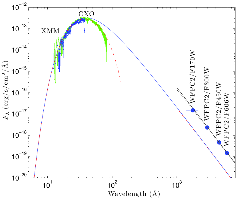
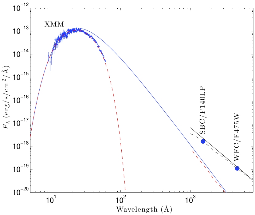
Figure 1.— X-ray to optical SEDs of RX J1856.5$-$3754 (left) and RX J2143.0+0654 (right). We plot archival X-ray data from XMM (blue) and CXO (green) along with the best-fit models (dashed red lines); the model for RX J1856.5$-$3754 is just a blackbody (Burwitz et al., 2003) while that for RX J2143.0+0654 includes a broad absorption line (Kaplan & van Kerkwijk, 2009b). The unabsorbed models are the solid blue lines. In the optical/UV we plot the HST data from van Kerkwijk & Kulkarni (2001) and this paper along with the best-fit power-law: the absorbed power-law is the black dashed line, while the unabsorbed power-law is the solid black line.

2.1. Image Reduction and Combination

The data for each of the five targets consist of multiple exposures covering the SDSS $g^{\prime}$ band (F475W filter, centered near 4700 Å) with the Advanced Camera for Surveys (ACS) Wide Field Channel (WFC) and the near-UV (F140LP filter, centered near 1500 Å) with the ACS Solar Blind Channel (SBC). For both the WFC and SBC data we used four sub-pixel dithered exposures per orbit and 1–3 orbits per object; for the WFC the object was placed at the center of the WFC1 detector so that we did not have to deal with the gap between the detectors. For completeness, we also re-analyzed the ACS/WFC F606W data on RX J1605.3+3249, since no photometry is given in the original publication by Zane et al. (2006).

WFC images obtained after Servicing Mission 4 (SM4) show charge trails along the CCD columns and faint stripes along the rows. The charge trails are due to the CCDs’ degrading charge transfer efficiency (CTE), while the stripes reflect a problem in the new electronics. These artifacts can significantly affect the detection of very faint sources as well as photometry and astrometry. We used the tasks acs_destripe (version 0.2.1) and CteCorr (also version 0.2.1, with the reference file pctefile_101109.fits; see Anderson & Bedin 2010) to correct the images, finding noticeably improvements in appearance. Checking the resulting photometry against that of raw images, we confirmed the conclusions of Anderson & Bedin (2010) that their algorithm restores photometric accuracy. Comparing against the average CTE corrections computed by Chiaberge et al. (2009), we found good agreement, although with some scatter (again, similar to what was found by Anderson & Bedin 2010). For the F606W data on RX J1605.3+3249, taken before SM4, the stripes are not present and we could not use the pixel-based CTE correction since the data were taken before SM4 and would require different calibration parameters, but other methods are possible to correct the reduced CTE losses. The SBC data do not suffer from such artifacts.

For each source in Table 1, ‘destriped’ and CTE-corrected (as necessary) images were drizzled using multidrizzle (Koekemoer et al., 2002) onto a single image. We experimented with the drizzle parameters to balance resolution and uniformity of sampling, settling on a set that gave good image quality: for the WFC data we used a final pixel scale of $0.04\arcsec{\rm pixel}^{-1}$ and a pixel fraction of 0.9, while for SBC we used a pixel scale of $0.03\arcsec{\rm pixel}^{-1}$ and a pixel fraction of 0.9. We verified that our photometry did not depend on the choices that we made.

2.2. Astrometry and Counterpart Identification

For all INSs, the SBC images show an obvious, rather bright counterpart, with at best a few other faint sources present. In contrast, in the WFC images, the counterparts are faint and there are many other, brighter stars. Previous identification of optical counterparts to the INSs has relied on absolute astrometry using the positions measured in X-rays and approximate ties between the X-ray and optical coordinate systems (e.g., Kaplan et al., 2003a). This can lead to uncertainties, as the absolute X-ray positions are typically accurate to only $0\farcs 6$ or so. However, the SBC images allow us to conclusively identify the counterparts with much higher accuracy. To do so we started by registering the SBC and WFC images. In two cases, we estimated offsets from single, bright optical stars that had faint ultraviolet counterparts, while in the others we relied on diffuse emission from galaxies (smoothing the SBC and WFC data as necessary to isolate a single bright component).

In all cases the registration was unambiguous, and led to clear identifications of the optical counterparts to the INSs. The SBC and WFC positions matched to within $<0\farcs 04$ (since they were taken at most 7 months apart, a typical proper motion of $100\,{\rm mas\,yr}^{-1}$ would lead to a comparable intrinsic offset).

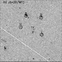
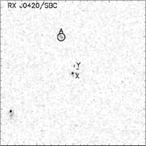
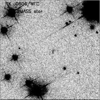
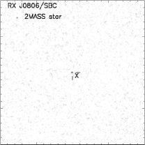
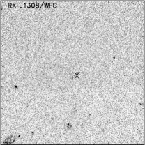
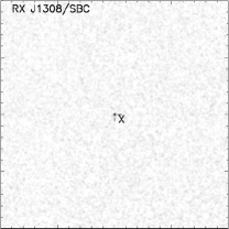
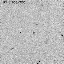
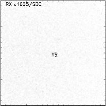
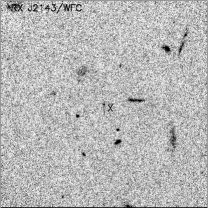
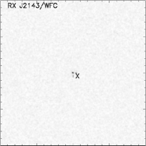
Figure 2.— ACS images of the fields around RX J0420.0$-$5022 (top left), RX J0806.4$-$4123 (top right), RX J1308.6+2127 (center left), RX J1605.3+3249 (center right), and RX J2143.0+0654 (bottom). For each source we plot WFC/F475W and SBC/F140LP images. The optical counterparts are labeled with “X”’s; their positions agree to better than $0\farcs 05$ with bright sources in the SBC/F140LP images. For RX J0420.0$-$5022, selected reference sources from Haberl, Pietsch, & Motch (1999) are labeled. The positions of objects “A” and a galaxy to the south-east match between the optical and UV images. For RX J0806.4$-$4123, the bright star to the north-east (2MASS J08062407$-$412223.1) is present on both images with the same position. North is up, and east is to the left, and the images are $20\arcsec\times 20\arcsec$. The SBC images have been smoothed with a Gaussian kernel with $\sigma=2$ pixels.

For all of the WFC images, we then registered the astrometry to 2MASS (Skrutskie et al., 2006). We fit for a shift only, leaving the plate-scale and rotation as set by the drizzling software. In the case of RX J0806.4$-$4123, we used 49 stars, restricted to being on the same detector (WFC1) as the presumed counterpart. For the other images, many fewer stars were available, and we used between 1 and 4 (all unsaturated and with stellar profiles). From the star-to-star variations, we infer that our absolute astrometry is accurate to $\sim\!0\farcs 2$ only, but this suffices to show that the positions of the identified counterparts agreed with published X-ray positions (and generally with previous identifications; see Sect. 3). We defer more accurate relative and absolute astrometry to a later paper.

Table 2X-ray Blackbodies for the INSs

RX J	$N_{\rm H}$	$kT$	$R/d$	Ref.	Notes
	($\times 10^{20}\,{\rm cm}^{-2}$)	(eV)	(${\rm km\,kpc}^{-1}$)
0420.0$-$5022	$2.02\pm 0.71$	$\phantom{0}45.0\pm 2.6$	$12.2\pm 0.2$	1	Normalization is from a blackbody fit.
0720.0$-$3125	$1.04\pm 0.02$	$\phantom{0}88.4\pm 0.4$	$15.7\pm 0.2$	2	From 2002-Nov, using XMM/EPIC
0806.4$-$4123	0$1.7\pm 0.2$0	$\phantom{0}87.2\pm 1.1$	$\phantom{0}9.6\pm 0.6$	3	Blackbody with 2 Gaussians
1308.6+2127	$\phantom{0}1.8\pm 0.2\phantom{0}$	$\phantom{0}\phantom{.}102\pm 2\phantom{.}\phantom{0}$	$\phantom{0}\phantom{0}\phantom{.}8\pm 2\phantom{.}\phantom{0}$	4	Normalization recomputed from Chandra/LETG
1605.3+3249	$0.98\pm 0.19$	$\phantom{0}92.6\pm 0.8$	$12.0\pm 0.6$	5	Blackbody with 1 Gaussian in wavelength, XMM/EPIC
1856.5$-$3754	$0.95\pm 0.03$	$\phantom{0}63.5\pm 0.2$	$36.7\pm 0.8$	6
2143.0+0654	$2.28\pm 0.09$	$104.0\pm 0.4$	$\phantom{0}6.2\pm 0.1$	7

Note. — The normalization and temperature are as viewed by an observer at infinity. Where multiple spectral fits are given in a paper, we try to be specific about which we have selected. While the best-fit spectra in many cases include absorption components, we only list the relevant blackbody parameters here.

References. — 1: Haberl et al. (2004); 2: Hohle et al. (2009); 3: Kaplan & van Kerkwijk (2009b); 4: Schwope et al. (2007); 5: van Kerkwijk et al. (2004); 6: Burwitz et al. (2003); 7: Kaplan & van Kerkwijk (2009a).

2.3. Photometry

We carried out aperture photometry of the final drizzled images using standard procedures in IRAF. For the WFC data, we used an aperture of $0\farcs 2$, and measured the sky between radii of $0\farcs 4$ and $0\farcs 8$ (for comparison, the effective FWHM in our drizzled images is $0\farcs 1$). Based on Sirianni et al. (2005), the aperture correction from $0\farcs 2$ to infinite radius for the F475W filter is $0.183$ mag. There is a small correction to our aperture correction, since some of the light from the stellar PSF will appear in the sky annulus. This will bias the sky value upward and hence make the source appear fainter than it is. The fraction of the stellar light in the sky annulus is 0.04 mag, based on Sirianni et al. (2005). Given the ratio between the areas of the source aperture and the sky annulus, the implied bias to our photometry is 0.003 mag, considerably less than our photometric uncertainty. For F606W, we proceeded similarly, except since we could not use the CTE correction of Anderson & Bedin (2010) on those data, we applied an empirical correction of 0.034 mag to the photometry, as inferred from the work of Chiaberge et al. (2009).

For the SBC data our procedure was similar. We estimated the sky background by computing a mean of the data between radii of $1\farcs 2$ and $2\farcs 4$; here, we found it necessary to turn off the default clipping of outliers, as this removed valid data: the sky is so dark that pixels contain only one or two counts, leading to a highly non-Gaussian distribution of sky values. Source photometry was done within a radius of $0\farcs 24$, and we used an aperture correction of $0.33$ mag, based on the work of Proffitt et al. (2003). Given the large aperture correction and the possibility of scattered light beyond $1\arcsec$, we include a 5% systematic uncertainty on our SBC photometry based on the scatter between the PSFs of the different objects. The final photometry are given in Table 1. All photometry is in the STMAG system, which is defined so that a source of constant $F_{\lambda}$ has a constant magnitude: ${\rm STMAG}=-2.5\log_{10}F_{\lambda}-21.1$ with $F_{\lambda}$ in ${\rm erg\,cm^{-2}\,s^{-1}\,\AA^{-1}}$.

3. Counterpart Identification and Spectral Fitting

We show the images for all sources in Figure 2. As discussed above, in all cases there are faint optical sources at the positions of the ultraviolet sources, whose positions also agree with the X-ray positions. Thus, our identifications are secure. Below, we first compare our results with previous work, and then discuss the ultraviolet and optical fluxes, both on their own and in relation to X-ray measurements.

RX J0420.0$-$5022

Haberl et al. (2004) identified a possible counterpart, which is roughly consistent in position. However, at $B=26.6\pm 0.3$, it is almost a magnitude brighter than our counterpart (using a correction from STMAG to Vega-based $B$-band of $m_{\rm F475W}-B=-0.26$, computed using synphot for a Rayleigh-Jeans spectrum; this should be accurate to better than 1%). It may be that the object identified by Haberl et al. (2004) was a blend of the true counterpart and another object of similar brightness about $0\farcs 5$ to the North (labeled “Y” in Figure 2, although it is hard to see in that image). Our photometry is much more consistent with the object proposed by Mignani et al. (2009).

RX J1308.6+2127

Kaplan, Kulkarni, & van Kerkwijk (2002a) identified the same counterpart as we did. Using STIS with no filter, which gives a broad band centered near 4200 Å, they measured $m_{\rm 50CCD}=28.56\pm 0.13$. Given $m_{\rm 50CCD}-m_{\rm F475W}=0.36\,$mag (again, using synphot), this is consistent with our photometry.

RX J1605.3+3249

While the counterpart is secure based on both colors and proper motion (Kaplan et al., 2003a; Motch et al., 2005; Zane et al., 2006), there is some question regarding the optical photometry, with Zane et al. (2006) arguing the it cannot be fit with a single power law. We do not confirm this: with our re-analysis of the F606W data, the space-based photometry is consistent with a power law (see below). For the ground-based observations of Motch et al. (2005), only the $R$-band point is consistent with what we measure ($B=27.22\pm 0.10$ and $R=26.9\pm 0.14$, and, using synphot, $m_{\rm F475W}-B=-0.32$ mag and $m_{\rm F606W}-R=0.23$).

RX J2143.0+0654

We identify the same object as that found by Zane et al. (2008) and Schwope et al. (2009). These authors each present $B$-band measurements, of $B=27.4\pm 0.2$ and $26.96\pm 0.20$, respectively. These are only marginally consistent; our measurement is more consistent with the latter. Mignani et al. (2011) set an upper limit of $R\gtrsim 27$, which is a bit fainter than our expected value of $R\approx 26.6$ (from synphot we find $m_{\rm 475W}-R=-0.26$ mag). These discrepancies may be from calibration uncertainties (Mignani et al. 2011 found the two $B$-band measurements to be consistent given uncertainties in atmospheric extinction correction), but at least for this source we cannot yet rule out variability or spectral curvature.

Overall, our identifications our consistent with prior ones, but some of the fluxes are discrepant. We do not undertake here to resolve this, but note that there is no evidence for variability or non-power-law optical-UV SEDs in the HST data we use below. We suspect that the discrepancies reflect mostly the more than usual care required to obtain reliable ground-based measurements for very faint objects (see, e.g., the discussion for RX J0720.4$-$3125 in Motch et al. 2003).

3.1. Power-law Fits

As in van Kerkwijk & Kulkarni (2001) and similar papers, we tried fitting single power-laws to just the optical/UV data for all 7 INSs; we included the space-based photometry for RX J1856.5$-$3754  (van Kerkwijk & Kulkarni, 2001) and for RX J0720.4$-$3125 (Kaplan et al., 2003b). Detailed fitting of HST data for the INSs presents some difficulties, since the zero-point fluxes were determined for a spectrum that is flat in $F_{\lambda}$, while the INSs have much steeper spectra. Given the often very wide bandpasses used, this leads to substantial changes in effective wavelength.

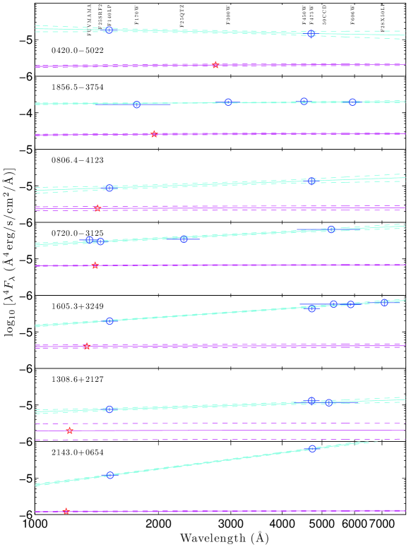
Figure 3.— Optical/UV SEDs for the 7 INSs. For each object (sorted by increasing $kT$ from top to bottom), we plot $\lambda^{4}F_{\lambda}$ versus wavelength; a Rayleigh-Jeans tail would be flat. The best-fit power-laws with $\pm 1\sigma$ uncertainties are shown by the cyan lines. The extrapolations of the X-ray blackbodies with $\pm 1\sigma$ uncertainties are shown by the magenta lines. The fluxes have been corrected for absorption using the nominal values of $N_{\rm H}$ from Table 2.2. The red stars show the wavelength of $10kT$. The different filters are labeled at the bottom.

To circumvent these difficulties, we relied on synphot to compute the expected STMAG as a function of extinction $A_{V}$ and power-law index $\alpha$ (with $F_{\lambda}\propto\lambda^{-\alpha}$, where a Rayleigh-Jeans spectrum would have $\alpha=4$) on a fine grid, with steps 0.005 mag in $A_{V}$ and 0.025 in $\alpha$. Then, for each object, we fitted a power law, optimizing for $\alpha$ and normalization, but keeping the reddening $A_{V}$ fixed to the value implied by the column density $N_{\rm H}$ determined from fits to the X-ray spectrum: $A_{V}=N_{\rm H}/1.79\times 10^{21}\,{\rm cm}^{-2}$ (Predehl & Schmitt 1995; note that this relation varies for different sight lines, but the extinction is small enough that the variations do not influence our results qualitatively, as we show below). We use the extinction curve of Cardelli, Clayton, & Mathis (1989), implemented as gal3 in synphot, and we assume $E(B-V)=A_{V}/3.1$. We note that we cannot fit uniquely for $A_{V}$ based only on our data, as the amount of reddening is highly degenerate with the power-law index. The exact value of $N_{\rm H}$ (and hence $A_{V}$) that we used depends somewhat on the calibration of the X-ray data and on the assumed spectral model, and could change in the future. We discuss this explicitly below.

The results of our power-law fits are shown in with Table 5 and Figure 3. Our uncertainties and $\chi^{2}$ values include a 5% systematic uncertainty for the F140LP data, owing to uncertainties in the aperture correction. For those objects with only two measurements we are left with a fully constrained fit (0 degrees-of-freedom); for the others, $\chi^{2}$ is consistent with a good fit.

The precise results depend slightly on our choice of extinction, but the results do not change qualitatively, since the extinctions inferred from the X-ray column densities are small ($A_{V}\lesssim 0.1\,$mag, and thus $A_{1400}\lesssim 0.3\,$mag). Indeed, given the quoted uncertainties on $N_{\rm H}$, the changes are nearly negligible. Somewhat larger systematic changes are possible from changes in the reddening law, the ratio of $N_{\rm H}$ to $A_{V}$, or the assumed X-ray spectral model. Therefore, in Table 5 we also give $d\alpha/dA_{V}$: the change in the power-law slope with changes in extinction (see also van Kerkwijk & Kulkarni 2001). We note, though, that even a 50% change in $A_{V}$ would generally change $\alpha$ by less than 0.1.

3.2. Comparison with X-ray Spectra

One of the main purposes of our work is to establish reliable estimates of the “optical excess,” the factor by which the optical/UV flux of the INS exceed the extrapolation of the X-ray blackbodies. To do this, we have collected the best-fit X-ray spectra for all 7 INSs in Table 2.2. In most cases the best-fit spectra are not purely blackbodies, but for the purposes of extrapolation the blackbody component is sufficient. We note that the spectrum of RX J0720.4$-$3125 changed during 2003 (de Vries et al., 2004). While there is no evidence that the optical flux of RX J0720.4$-$3125 changed during that time (Kaplan, van Kerkwijk, & Anderson, 2007), the two different X-ray spectra differ by a factor of 1.54 from each other, thus introducing a systematic uncertainty into our inferred optical/UV excess. It does not, however, affect the shape of the excess, as the HST data are well into the Rayleigh-Jeans tail and uncertainties in the extinction are small.

For all of the objects we determine the excess relative to expected fluxes calculated by passing the extrapolated, reddened X-ray spectrum through the HST filter response curves, using synphot. This avoids issues of uncertainties in the effective wavelengths or zero-point flux that come from using spectra that differ significantly in slope from the calibration spectra. We determined formal uncertainties by repeating the above for values that differ by 1-$\sigma$ in all parameters from the best-fit spectrum, taking as 1-$\sigma$ uncertainties on the extrapolated magnitudes the maximum and minimum of these variations.

We list our results in Tables 3 and 4. For completeness, we include expected values for instrument/filter/object combinations beyond those used here, and also give reference photometry for an unabsorbed $10^{6}\,$K blackbody as well as approximate values for the wavelength-dependent extinction $A_{\lambda}/A_{V}$ (see van Kerkwijk & Kulkarni 2001 for an extended discussion). The extinction values actually depend slightly on the value of the overall extinction $A_{V}$, since this changes the shape of the spectrum and hence the integral over the filter response. The effect is largest for the widest filters, like STIS/50CCD. However, for the range of extinction values considered here ($N_{\rm H}=(1-4)\times 10^{20}\,{\rm cm}^{-2}$ corresponds to $A_{V}\approx 0.06-0.22$), the changes are less than 1% in $A_{\lambda}/A_{V}$.

Along with the more easily assessed uncertainties on $kT$ and $(R/d)$, a possibly significant systematic uncertainty in our model is variations in extinction. Similar to the analysis above, we explore this issue by considering a $\pm 50$% range on $A_{V}$ around the nominal value. This results in uncertainties on the extrapolated photometry ranging from 0.09 mag (for the shortest wavelengths) to 0.03 mag (for the longest), based on a fiducial $N_{\rm H}=10^{20}\,{\rm cm}^{-2}$. For other values of $N_{\rm H}$, the uncertainties are proportionate. Generally, these additional uncertainties are smaller than the photometric uncertainties, and will not affect our results. The measured excesses are given in Table 5 and Figure 3.

Table 3Predicted HST UV Photometry from Extrapolated X-ray Blackbodies

RX J	Extrapolated STMAG
	STIS/FUV	STIS/FUV	ACS/SBC	WFPC2	STIS/NUV
		F25SrF2	F140LP	F170W	F25Qtz
0420.0$-$5022	$24.87\pm 0.07$	$25.10\pm 0.07$	$25.30\pm 0.07$	$25.95\pm 0.07$	$27.03\pm 0.07$
0720.0$-$3125	$23.36\pm 0.03$	$23.61\pm 0.03$	$23.82\pm 0.03$	$24.48\pm 0.03$	$25.57\pm 0.03$
0806.4$-$4123	$24.57\pm 0.14$	$24.81\pm 0.14$	$25.01\pm 0.14$	$25.67\pm 0.14$	$26.76\pm 0.14$
1308.6+2127	$24.79\pm 0.55$	$25.03\pm 0.55$	$25.24\pm 0.55$	$25.89\pm 0.55$	$26.99\pm 0.55$
1605.3+3249	$23.88\pm 0.11$	$24.13\pm 0.11$	$24.34\pm 0.11$	$25.00\pm 0.11$	$26.09\pm 0.11$
1856.5$-$3754	$21.88\pm 0.05$	$22.13\pm 0.05$	$22.34\pm 0.05$	$23.00\pm 0.05$	$24.09\pm 0.05$
2143.0+0654	$25.41\pm 0.03$	$25.64\pm 0.03$	$25.84\pm 0.03$	$26.50\pm 0.03$	$27.59\pm 0.03$
$10^{6}$ K	19.81	20.08	20.29	20.96	22.05
$\lambda_{\rm eff}$ (Å)	1355	1442	1517	1769	2283
$A_{\lambda}/A_{V}$	3.11	2.84	2.71	2.65	2.58

Note. — We give the instrument name and filter for all UV observations that we consider; not all objects were observed with all combinations, and see Table 4 for the optical observations. The 1-$\sigma$ uncertainties are based on the uncertainties in the X-ray spectra (Table 2.2) and do not include any other systematic terms.

Table 4Predicted HST Optical Photometry from Extrapolated X-ray Blackbodies

RX J	Extrapolated STMAG
	WFPC2	WFPC2	ACS/WFC	STIS/CCD	ACS/WFC	WFPC2	STIS/CCD
	F300W	F450W	F475W	50CCD	F606W	F606W	F28x50LP
0420.0$-$5022	$28.06\pm 0.07$	$29.81\pm 0.06$	$29.98\pm 0.06$	$30.35\pm 0.07$	$30.88\pm 0.06$	$30.95\pm 0.06$	$31.66\pm 0.06$
0720.0$-$3125	$26.64\pm 0.03$	$28.44\pm 0.03$	$28.62\pm 0.03$	$28.96\pm 0.03$	$29.54\pm 0.03$	$29.60\pm 0.03$	$30.32\pm 0.03$
0806.4$-$4123	$27.81\pm 0.14$	$29.59\pm 0.14$	$29.76\pm 0.14$	$30.11\pm 0.14$	$30.67\pm 0.14$	$30.73\pm 0.14$	$31.45\pm 0.14$
1308.6+2127	$28.03\pm 0.55$	$29.81\pm 0.55$	$29.98\pm 0.55$	$30.33\pm 0.55$	$30.89\pm 0.55$	$30.95\pm 0.55$	$31.67\pm 0.55$
1605.3+3249	$27.17\pm 0.11$	$28.97\pm 0.11$	$29.15\pm 0.11$	$29.49\pm 0.11$	$30.07\pm 0.11$	$30.13\pm 0.11$	$30.85\pm 0.11$
1856.5$-$3754	$25.16\pm 0.05$	$26.96\pm 0.05$	$27.13\pm 0.05$	$27.48\pm 0.05$	$28.05\pm 0.05$	$28.12\pm 0.05$	$28.84\pm 0.05$
2143.0+0654	$28.62\pm 0.03$	$30.37\pm 0.03$	$30.54\pm 0.03$	$30.91\pm 0.03$	$31.44\pm 0.03$	$31.51\pm 0.03$	$32.22\pm 0.03$
$10^{6}$ K	23.16	25.00	25.18	25.50	26.11	26.18	26.91
$\lambda_{\rm eff}$ (Å)	2955	4520	4709	5066	5844	5932	7025
$A_{\lambda}/A_{V}$	1.93	1.30	1.24	1.58	0.97	0.95	0.79

Note. — We give the instrument name and filter for all optical observations that we consider; not all objects were observed with all combinations, and see Table 3 for the optical observations. The 1-$\sigma$ uncertainties are based on the uncertainties in the X-ray spectra (Table 2.2) and do not include any other systematic terms.

4. Discussion & Conclusions

4.1. Comparing the INSs to Each Other

It is clear that there is a wide variation in both the normalization and slope of the optical/UV power-laws for the INSs. Comparing to previous work, we confirm the conclusion of van Kerkwijk & Kulkarni (2001) that RX J1856.5$-$3754 has a nearly thermal spectrum, close to $F_{\lambda}\propto\lambda^{-4}$, while the spectrum of RX J0720.4$-$3125 is somewhat flatter, consistent with what was found by Kaplan et al. (2003b) and Motch et al. (2003). The other objects extend the range, with RX J0420.0$-$5022 also appearing thermal and RX J2143.0+0654, with $\alpha=2.5$, having the flattest, least Rayleigh-Jeans-like spectrum (as well as the highest excess; see below). No source has a slope that is significantly steeper than Rayleigh-Jeans.

Comparing the emission to the X-ray spectrum, there is a similarly wide variation in both the amount and slope of the optical/UV excess: most sources are not consistent with the constant excess of RX J1856.5$-$3754, and the amount of the excess varies significantly, although no source has measurements below its X-ray extrapolation. At 1500 Å the range is from about 3.5 to almost 10, with statistically significant variation ($\chi^{2}=134$ for 6 DOF) even when excluding RX J2143.0+0654 ($\chi^{2}=46$ for 5 DOF). At longer wavelengths the variation is even larger, going from 6 to 50 at 4700 Å. Here, RX J2143.0+0654 is clearly very different from the rest, but again when excluding it there is still significant variation ($\chi^{2}=21$ for 5 DOF). These are beyond deviations possible from the X-ray uncertainties, and while X-ray calibration errors, differences in X-ray fitting methodology, and variability can all contribute to variations in the excess, as noted above the shape of the excess is robust. See Figure 1 for a full optical-to-X-ray comparison of RX J1856.5$-$3754 and RX J2143.0+0654.

If the X-ray and optical came from different regions on the surface (Braje & Romani, 2002), we might expect variations in the excess to correlate with changes in the X-ray pulsed fraction, as both would be dependent on geometry: a small X-ray hotspot would give rise to both a large optical excess and a large pulsed fraction. Some allowances could be made for viewing angles, but with 7 sources this would start to average out. However, we do not see any such correlation. As an example, both RX J1856.5$-$3754 and RX J0420.0$-$5022 have similar optical excesses, but the pulsed fraction for RX J1856.5$-$3754 is about 1% (Tiengo & Mereghetti, 2007) while that of RX J0420.0$-$5022 is 13% (Haberl et al., 2004), and RX J1605.3+3249 has a larger excess but a small pulsed fraction.

Even so, we can still fit the optical/UV SEDs as part of some blackbody, with radius and temperature free (Fig. 4). For RX J1856.5$-$3754 this is largely degenerate (since it looks like a Rayleigh-Jeans), but for other sources the temperature and hence the radius are constrained. Some of these (mostly RX J0420.0$-$5022) are not likely based on extrapolations to the X-ray band, as they would exceed the flux at 100 eV. All fits are generally consistent with reduced $\chi^{2}\approx 1$, although there are not many degrees of freedom. This fit gives a normalization of $R/d\approx 400\,{\rm km\,kpc}^{-1}$ for RX J2143.0+0654. Since we expect a distance to RX J2143.0+0654 of 500–1000 pc based on the X-ray spectrum, this would imply a rather large radius if it is interpreted physically, and may only apply in light of the scattering model discussed below. Most of the objects fall on a single locus with radius increasing as the temperature decreases. Much of this just comes from keeping a similar excess among the sources (we would expect $R^{2}\propto 1/T$), but it is clear that RX J1605.3+3249 and RX J2143.0+0654 are inconsistent with the other objects.

We saw above that the optical excess does not appear to correlate with the X-ray pulsed fraction, suggesting that a model like Braje & Romani (2002) is incomplete. Taking the basic spectral parameters ($kT$ along with energy of the absorption lines) and the basic rotational parameter (pulsed fraction, magnetic field, spin-down luminosity) we see no clear trends with the optical/UV properties that we have measured here. The one possible exception is in relating the spectral index to $kT$: in Figure 5 it appears that the hotter objects have smaller spectral indices. Much of this correlation comes from RX J2143.0+0654, but even without it the correlation appears somewhat significant: Spearman’s rank correlation coefficient (Press et al., 1992, p. 641) for all objects is $-0.75$ with a null-hypothesis probability of 5%, and this drops to $-0.6$ (21% null hypothesis probability) when RX J2143.0+0654 is excluded. For the small number of objects considered here, this is reasonable but not definitive.

Such a correlation may imply that the SEDs of all of the INSs deviate from a Rayleigh-Jeans tail, but that the energy at which they do it depends on their temperatures. For the cool RX J1856.5$-$3754 and RX J0420.0$-$5022, the optical/UV window still seems thermal. But for the hotter RX J1308.6+2127 and RX J2143.0+0654, the thermal portion would be lost shortward of 1000 Å. The shift does not appear linear, as measuring the excess at a wavelength that scales with $1/kT$ does not improve the agreement among objects.

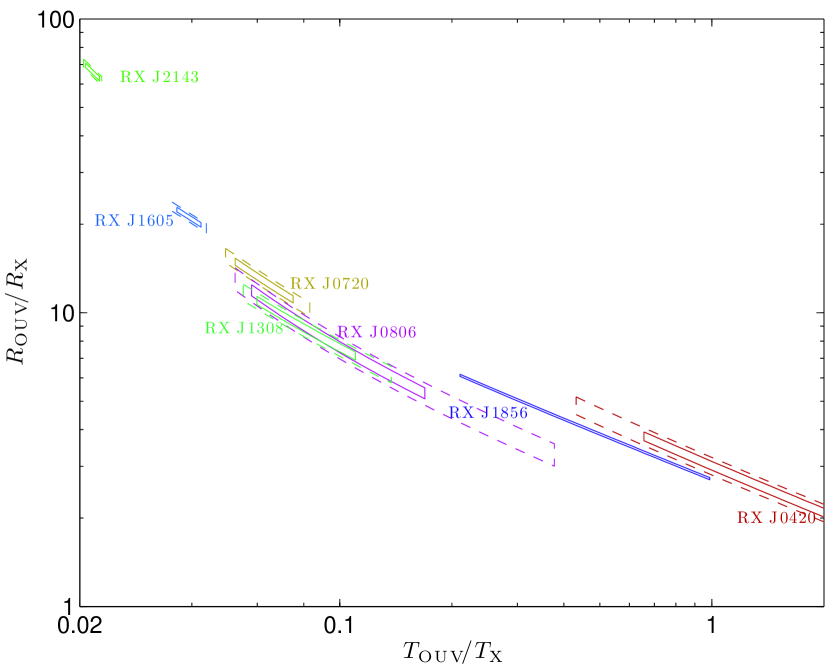
Figure 4.— Results of fitting blackbodies to only the optical/UV data for the INSs. We show $\pm 1\sigma$ (solid) and $\pm 2\sigma$ (dashed) limits on the temperature and normalization $R/d$, where in both cases we scale the fitted values by the values measured in X-rays (causing the distances to cancel). Individual sources are labeled. For RX J1856.5$-$3754 and RX J0420.0$-$5022, the results are consistent with the X-ray temperature at a constant excess, as seen from Table 5. Other objects have flatter spectra so the implied fits are cooler. For the objects with more than two data points and $T_{\rm OUV}<T_{\rm X}$, RX J0720.4$-$3125 has $\chi^{2}=4.3$ (2 DOF) and RX J1605.3+3249 has $\chi^{2}=5.2$ (3 DOF). Extrapolating the optical fits to higher energies for RX J0420.0$-$5022 and to a lesser extent RX J1856.5$-$3754 might not be consistent with the X-ray data.

In contrast to some previous attempts to measure the optical SED using both ground- and space-based measurements, we see that all INSs are well fit by a single power-law. Further, our results using only HST data are similar to those for RX J1856.5$-$3754 and RX J0720.4$-$3125 that include ground-based data. Our conclusions regarding the 5 sources observed here are relatively insensitive to $\sim$month scale variability, as in many (but not all) of the cases the optical and UV observations occurred within weeks of each other, but this is not always the case. For instance, RX J1605.3+3249 now has more HST photometry than RX J1856.5$-$3754 spanning almost 10 years, but still appears smooth. Whether this implies that the optical/UV is constant or just that we are unlucky is not clear, but future high-quality measurements should be able to address this.

4.2. Comparing the INSs to Pulsars and Magnetars

Previous modeling of RX J0720.4$-$3125 (Kaplan et al., 2003b) could not distinguish between a single non-thermal power-law and a combination of power-laws. Unfortunately, with our new data it is still hard to make that distinction, as the wide wavelength gap between the optical and UV even in the best case (RX J1605.3+3249) could easily hide a curved SED. Future observations in the 2000–3000 Å range might help better constrain such spectra and settle this question. We note, though, while the sources with few data-points can accommodate a power-law as flat as that for RX J2143.0+0654 in addition to a steeper, thermal component, objects with denser coverage like RX J0720.4$-$3125 and RX J1605.3+3249 cannot.

We can set rough upper limits on another power-law by requiring that any non-thermal contribution match our reddest optical point as well as be below the X-ray black body at 1.5 keV, where typically there are no more counts (Figure 1). We also require that such a power-law have a slope such that it is falling in photons per unit energy toward higher energies, so that it stays hidden (see Kaplan et al., 2003b). Taken together with the parallax for RX J1856.5$-$3754 (Walter et al., 2010) and assuming all the INSs have similar radii, we find non-thermal luminosities integrated over the 2–10 keV band of typically $10^{28-30}\,{\rm erg\,s}^{-1}$. At the upper end we do not believe that such luminosities could be real, as they would be close to 100% of $\dot{E}$, in contrast to radio pulsars that have non-thermal luminosities of $\sim 10^{-3}\dot{E}$ in X-rays (Becker & Trümper, 1997). Even without such an extrapolation our optical luminosities ($(0.3-1.7)\times 10^{29}\,{\rm erg\,s}^{-1}$) are uncomfortably high for a typical magnetospheric origin, since it would be $>10^{-3}\dot{E}$ compared to typical values of ratios of $10^{-7}$–$10^{-6}$ for radio pulsars (Zavlin & Pavlov, 2004). However, while the X-ray emission cannot be powered by $\dot{E}$ (since X-ray luminosities are $\gg\dot{E}$; Kaplan & van Kerkwijk 2009a) some amount of the optical emission could be related, albeit with a different mechanism than that which usually operates for pulsars.

If the deviations from a thermal SED were from magnetospheric emission as in pulsars (Pavlov et al., 1997; Shibanov et al., 2005; Kargaltsev et al., 2005), we might expect a correlation in the amount of the excess or the optical luminosity with the spin-down luminosity $\dot{E}$, as this is what drives the X-ray power-laws seen in pulsars and may drive the optical too. Again, though, we see no such correlation.

The behavior of the INSs also deviates from what is seen in the cases of other relatively young neutron stars in the optical, namely magnetars (Mereghetti, 2008). Most magnetars have only been seen in the infrared (likely due to high extinctions). The infrared emission is variable, and may or may not be linked to the X-ray emission. The one source with confirmed optical emission is 4U 0142+61 (Hulleman, van Kerkwijk, & Kulkarni, 2000, 2004). The optical emission is known to pulse at the X-ray period (Kern & Martin, 2002; Dhillon et al., 2005), suggesting that it is likely magnetospheric in origin (Zane, Nobili, & Turolla, 2011). Importantly for this comparison, the optical emission is not a single power-law (Hulleman et al., 2004). In contrast, the emission of the INSs is well fit by a single power-law and is (so far) constant in time. The flattening of the SED of RX J2143.0+0654 toward longer wavelengths is somewhat suggestive of the broadband SED of 4U 0142+61, but the other characteristics make it distinct.

It may be that the similarities with magnetars arise from a common origin, which suggests that the optical emission results from resonant scattering in the neutron stars’ magnetospheres Lyutikov & Gavriil (2006). However, qualitative differences between the INSs and magnetars exist: while the ranges overlap, the magnetars typically have higher values of magnetic to thermal energy $\hbar eB/m_{e}ckT$ ($\gtrsim 10^{4}$ for the magnetars vs. $\approx 3000$ for the INSs), and the higher fields of the magnetars mean that scattering and pair-production happen much more quickly. The optical emission of the INSs could instead be from an inverted temperature layer (like a chromosphere) that is driven by a twisted magnetosphere (C. Thompson 2011, pers. comm.). We note that for RX J2143.0+0654, which has the most extreme optical excess, we also see that the X-ray pulsations have odd harmonics likely indicative of a complex field geometry (Kaplan & van Kerkwijk, 2009b).

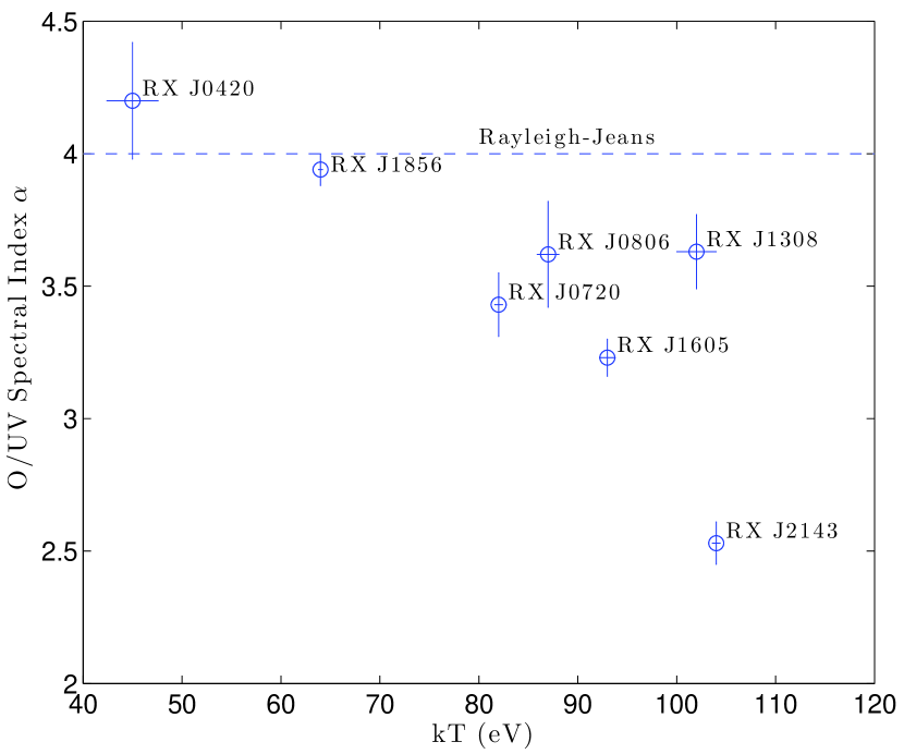
Figure 5.— Optical/UV spectral index ($\alpha$ from Table 5) versus X-ray temperature $kT$ (from Table 2.2) for the INSs. The horizontal line shows a slope of 4, to be expected for a Rayleigh-Jeans tail.

4.3. Atmosphere Models for the INSs

In the context of magnetized atmosphere models for neutron stars, the amount of optical/UV excess can depend on the magnetic field strength. Therefore we examined the UV/optical emission predicted by the NSMAX models of NS X-ray spectra constructed for Xspec (Ho et al., 2008); these models span the range $B=(1-30)\times 10^{12}$ G and $kT\sim 20-400$ eV for a partially ionized hydrogen atmosphere. We find that, although the magnitude of the flux differs from that of a blackbody, the wavelength dependence still exhibits a $\lambda^{-4}$ Rayleigh-Jeans behavior. Deviations from the Rayleigh-Jeans behavior occur as a result of the proton cyclotron line at (redshifted) $\sim 2500/B_{12}$ Å (with $B=10^{12}B_{12}$ G). For $B\lesssim 4\times 10^{12}$ G, the wings of the cyclotron line can reproduce the wavelength-behavior seen in Fig. 3, though not at the magnitude of RX J2143.0+0654; however, it is unclear how strongly this behavior depends on temperature (see Fig. 5). If the deviations from Rayleigh-Jeans are due to absorption in the wings of the proton cyclotron line, these spectrally-inferred magnetic fields are much lower than those inferred from timing (Kaplan & van Kerkwijk, 2009a). A factor of two increase in the former may be the result of a helium (rather than hydrogen) atmosphere. A possible discrepancy between timing and spectral magnetic fields may exist when considering the broad X-ray absorption features (Haberl, 2007; van Kerkwijk & Kaplan, 2007; Kaplan & van Kerkwijk, 2009b) but there it is in the opposite direction (the features are more consistent with strong fields), and hence easier to understand in terms of higher-order magnetic moments leading to locally stronger magnetic fields. We also note that our models indicate an increasing flux with increasing wavelength similar in magnitude to that seen in the INSs (again except for RX J2143.0+0654) for $kT\sim 100$ eV and magnetic fields more similar to what is seen in X-ray timing, $B\approx(2-3)\times 10^{13}$ G; the cause of this is still under investigation.

Table 5Power-law Fits to HST Photometry

RX J	$A_{V,\rm ref}$	$F_{\lambda}(2500\,{\rm\AA})$	Excess			$\alpha$	$d\alpha/dA_{V}$	$\chi^{2}$/DOF
	(mag)	($10^{-18}$ erg cm-2 s-1 Å-1)	1500 Å	2500 Å	4700 Å
0420.0$-$5022	0.11	$0.34\pm 0.03$	$9.6\pm 1.3$	0$8.3\pm 0.8$	0$7.2\pm 0.7$	$4.20\pm 0.22$	1.2	0/0
0720.0$-$3125	0.06	$0.92\pm 0.05$	$4.6\pm 0.3$	0$6.1\pm 0.4$	0$8.6\pm 0.5$	$3.43\pm 0.12$	1.4	1.5/20.
0806.4$-$4123	0.10	$0.22\pm 0.02$	$3.6\pm 0.6$	0$4.3\pm 0.7$	0$5.5\pm 0.9$	$3.62\pm 0.20$	1.2	0/0
1308.6+2127	0.10	$0.19\pm 0.01$	$3.8\pm 2.1$	0$4.5\pm 2.5$	0$5.6\pm 3.2$	$3.63\pm 0.14$	1.2	0.4/10.
1605.3+3249	0.05	$0.68\pm 0.02$	$5.0\pm 0.5$	0$7.2\pm 0.8$	$11.6\pm 1.3$	$3.23\pm 0.07$	1.3	3.5/30.
1856.5$-$3754	0.05	$4.25\pm 0.07$	$7.1\pm 0.4$	0$7.1\pm 0.3$	0$7.3\pm 0.3$	$3.94\pm 0.06$	1.9	2.6/20.
2143.0+0654	0.13	$0.48\pm 0.02$	$9.5\pm 0.4$	$19.9\pm 0.9$	$49.8\pm 2.3$	$2.53\pm 0.08$	1.2	0/0

Note. — We give the nominal extinction $A_{V,\rm ref}$ (computed from $N_{\rm H}$ in Table 2.2), the absorbed flux density at 2500 Å, the power-law index $\alpha$ (defined such that $F_{\lambda}\propto\lambda^{-\alpha}$), and the $\chi^{2}$ and degrees of freedom for the fit. We also list the excesses over the X-ray blackbody at 2500 Å (where the normalization is calculated) and at 1500 Å (appropriate for F140LP) and 4700 Å (appropriate for F475W). Uncertainties on the X-ray fits are included in the given uncertainties on the excess. Extinction at 2500 Å is taken as $A_{2500\,{\rm\AA}}/A_{V}=2.32$. We also give the change in power-law index with changes in extinction, $d\alpha/dA_{V}$, i.e., $\alpha(A_{V})=\alpha(A_{V,{\rm ref}})+d\alpha/dA_{V}(A_{V}-A_{V,{\rm ref}})$.

There exists an uncertainty in the models of strongly-magnetized NS atmospheres at long wavelengths. The plasma frequencies for the model atmospheres constructed in, e.g., Ho et al. (2008), lie near the optical/UV regime. Classically, emission below the plasma frequency should be suppressed, or at least highly modified. The suppression would be stronger at longer wavelengths (opposite to the behavior seen in Fig. 3), since the plasma frequency increases with density. Calculations using an ad-hoc approach to account for this dense plasma suppression (see Ho et al. 2003 for details) indicate that deviations from Rayleigh-Jeans occur at far-UV/soft X-rays (for the likely INS magnetic fields $B\gg 10^{12}$ G), while at optical wavelengths, the flux is suppressed but the wavelength-dependence is not affected. Thus the above considerations may still apply. Improvements on the treatment used here are possible (see, e.g., Brinkmann 1980; Turolla, Zane, & Drake 2004; Pérez-Azorín, Miralles, & Pons 2005; van Adelsberg et al. 2005; Ho et al. 2007) but do not qualitatively alter the results, while a fully self-consistent model of the emission properties of the condensed surface below the atmosphere is beyond the scope of this work.

Regardless of explanation, we have conclusively identified optical counterparts to all 7 INSs and shown that the relatively straightforward behavior shown by RX J1856.5$-$3754 is not necessarily the dominant behavior. Future modeling of these sources will have to account for this diversity. The quality of the HST data has allowed us to measure accurate SEDs and set references for future astrometry.

References

- Anderson & Bedin (2010) Anderson, J. & Bedin, L. R. 2010, PASP, 122, 1035
- Becker & Trümper (1997) Becker, W. & Trümper, J. 1997, A&A, 326, 682
- Braje & Romani (2002) Braje, T. M. & Romani, R. W. 2002, ApJ, 580, 1043
- Brinkmann (1980) Brinkmann, W. 1980, A&A, 82, 352
- Burwitz et al. (2003) Burwitz, V., Haberl, F., Neuhäuser, R., Predehl, P., Trümper, J., & Zavlin, V. E. 2003, A&A, 399, 1109
- Burwitz et al. (2001) Burwitz, V., Zavlin, V. E., Neuhäuser, R., Predehl, P., Trümper, J., & Brinkman, A. C. 2001, A&A, 379, L35
- Cardelli et al. (1989) Cardelli, J. A., Clayton, G. C., & Mathis, J. S. 1989, ApJ, 345, 245
- Chiaberge et al. (2009) Chiaberge, M., Lim, P. L., Kozhurina-Platais, V., Sirianni, M., & Mack, J. 2009, Updated CTE photometric correction for WFC and HRC, HST Instrument Status Report 09-01, Space Telescope Science Institute
- de Vries et al. (2004) de Vries, C. P., Vink, J., Méndez, M., & Verbunt, F. 2004, A&A, 415, L31
- Dhillon et al. (2005) Dhillon, V. S., Marsh, T. R., Hulleman, F., van Kerkwijk, M. H., Shearer, A., Littlefair, S. P., Gavriil, F. P., & Kaspi, V. M. 2005, MNRAS, 363, 609
- Drake et al. (2002) Drake, J. J. et al. 2002, ApJ, 572, 996
- Haberl (2007) Haberl, F. 2007, Ap&SS, 308, 181
- Haberl et al. (2004) Haberl, F., Motch, C., Zavlin, V. E., Reinsch, K., Gänsicke, B. T., Cropper, M., Schwope, A. D., Turolla, R., & Zane, S. 2004, A&A, 424, 635
- Haberl et al. (1999) Haberl, F., Pietsch, W., & Motch, C. 1999, A&A, 351, L53
- Haberl et al. (2006) Haberl, F., Turolla, R., de Vries, C. P., Zane, S., Vink, J., Méndez, M., & Verbunt, F. 2006, A&A, 451, L17
- Ho (2007) Ho, W. C. G. 2007, MNRAS, 380, 71
- Ho et al. (2007) Ho, W. C. G., Kaplan, D. L., Chang, P., van Adelsberg, M., & Potekhin, A. Y. 2007, MNRAS, 375, 821
- Ho et al. (2003) Ho, W. C. G., Lai, D., Potekhin, A. Y., & Chabrier, G. 2003, ApJ, 599, 1293
- Ho et al. (2008) Ho, W. C. G., Potekhin, A. Y., & Chabrier, G. 2008, ApJS, 178, 102
- Hohle et al. (2009) Hohle, M. M., Haberl, F., Vink, J., Turolla, R., Hambaryan, V., Zane, S., de Vries, C. P., & Méndez, M. 2009, A&A, 498, 811
- Hulleman et al. (2000) Hulleman, F., van Kerkwijk, M. H., & Kulkarni, S. R. 2000, Nature, 408, 689
- Hulleman et al. (2004) —. 2004, A&A, 416, 1037
- Kaplan (2008) Kaplan, D. L. 2008, AIPC, 983, 331, arXiv:0801.1143
- Kaplan et al. (2002a) Kaplan, D. L., Kulkarni, S. R., & van Kerkwijk, M. H. 2002a, ApJ, 579, L29
- Kaplan et al. (2003a) —. 2003a, ApJ, 588, L33
- Kaplan & van Kerkwijk (2009a) Kaplan, D. L. & van Kerkwijk, M. H. 2009a, ApJ, 705, 798
- Kaplan & van Kerkwijk (2009b) —. 2009b, ApJ, 692, L62
- Kaplan et al. (2002b) Kaplan, D. L., van Kerkwijk, M. H., & Anderson, J. 2002b, ApJ, 571, 447
- Kaplan et al. (2007) —. 2007, ApJ, 660, 1428
- Kaplan et al. (2003b) Kaplan, D. L., van Kerkwijk, M. H., Marshall, H. L., Jacoby, B. A., Kulkarni, S. R., & Frail, D. A. 2003b, ApJ, 590, 1008
- Kargaltsev et al. (2005) Kargaltsev, O. Y., Pavlov, G. G., Zavlin, V. E., & Romani, R. W. 2005, ApJ, 625, 307
- Kern & Martin (2002) Kern, B. & Martin, C. 2002, Nature, 417, 527
- Koekemoer et al. (2002) Koekemoer, A. M., Fruchter, A. S., Hook, R. N., & Hack, W. 2002, in The 2002 HST Calibration Workshop, ed. S. Arribas, A. Koekemoer, & B. Whitmore (Baltimore: Space Telescope Science Institute), 337
- Lattimer & Prakash (2007) Lattimer, J. M. & Prakash, M. 2007, Phys. Rep., 442, 109
- Lyutikov & Gavriil (2006) Lyutikov, M. & Gavriil, F. P. 2006, MNRAS, 368, 690
- Medin & Lai (2007) Medin, Z. & Lai, D. 2007, MNRAS, 382, 1833
- Mereghetti (2008) Mereghetti, S. 2008, A&A Rev., 15, 225
- Mignani et al. (2009) Mignani, R. P., Motch, C., Haberl, F., Zane, S., Turolla, R., & Schwope, A. 2009, A&A, 505, 707
- Mignani et al. (2011) Mignani, R. P., Zane, S., Turolla, R., Haberl, F., Cropper, M., Motch, C., Treves, A., & Zampieri, L. 2011, A&A, 530, A39+
- Motch et al. (2005) Motch, C., Sekiguchi, K., Haberl, F., Zavlin, V. E., Schwope, A., & Pakull, M. W. 2005, A&A, 429, 257
- Motch et al. (2003) Motch, C., Zavlin, V. E., & Haberl, F. 2003, A&A, 408, 323
- Page et al. (2006) Page, D., Turolla, R., & Zane, S., eds. 2006, Isolated Neutron Stars: from the Interior to the Surface (Springer)
- Pavlov et al. (1997) Pavlov, G. G., Welty, A. D., & Cordova, F. A. 1997, ApJ, 489, L75
- Pérez-Azorín et al. (2005) Pérez-Azorín, J. F., Miralles, J. A., & Pons, J. A. 2005, A&A, 433, 275
- Pires et al. (2009) Pires, A. M., Motch, C., Turolla, R., Treves, A., & Popov, S. B. 2009, A&A, 498, 233
- Predehl & Schmitt (1995) Predehl, P. & Schmitt, J. H. M. M. 1995, A&A, 293, 889
- Press et al. (1992) Press, W. H., Teukolsky, S. A., Vetterling, W. T., & Flannery, B. P. 1992, Numerical recipes in C. The art of scientific computing, 2nd edn. (Cambridge: University Press)
- Proffitt et al. (2003) Proffitt, C. R., Brown, T. M., Mobasher, B., & Davies, J. 2003, Absolute Flux Calibration of STIS MAMA Imaging Modes, HST Instrument Status Report 03-01, Space Telescope Science Institute
- Schwope et al. (2009) Schwope, A. D., Erben, T., Kohnert, J., Lamer, G., Steinmetz, M., Strassmeier, K., Zinnecker, H., Bechtold, J., Diolaiti, E., Fontana, A., Gallozzi, S., Giallongo, E., Ragazzoni, R., de Santis, C., & Testa, V. 2009, A&A, 499, 267
- Schwope et al. (2007) Schwope, A. D., Hambaryan, V., Haberl, F., & Motch, C. 2007, Ap&SS, 308, 619
- Shibanov et al. (2005) Shibanov, Y. A., Sollerman, J., Lundqvist, P., Gull, T., & Lindler, D. 2005, A&A, 440, 693
- Sirianni et al. (2005) Sirianni, M., Jee, M. J., Benítez, N., Blakeslee, J. P., Martel, A. R., Meurer, G., Clampin, M., De Marchi, G., Ford, H. C., Gilliland, R., Hartig, G. F., Illingworth, G. D., Mack, J., & McCann, W. J. 2005, PASP, 117, 1049
- Skrutskie et al. (2006) Skrutskie, M. F., Cutri, R. M., Stiening, R., Weinberg, M. D., Schneider, S., Carpenter, J. M., Beichman, C., Capps, R., Chester, T., Elias, J., Huchra, J., Liebert, J., Lonsdale, C., Monet, D. G., Price, S., Seitzer, P., Jarrett, T., Kirkpatrick, J. D., Gizis, J. E., Howard, E., Evans, T., Fowler, J., Fullmer, L., Hurt, R., Light, R., Kopan, E. L., Marsh, K. A., McCallon, H. L., Tam, R., Van Dyk, S., & Wheelock, S. 2006, AJ, 131, 1163
- Tiengo & Mereghetti (2007) Tiengo, A. & Mereghetti, S. 2007, ApJ, 657, L101
- Turolla et al. (2004) Turolla, R., Zane, S., & Drake, J. J. 2004, ApJ, 603, 265
- van Adelsberg et al. (2005) van Adelsberg, M., Lai, D., Potekhin, A. Y., & Arras, P. 2005, ApJ, 628, 902
- van Kerkwijk & Kaplan (2007) van Kerkwijk, M. H. & Kaplan, D. L. 2007, Ap&SS, 308, 191
- van Kerkwijk & Kaplan (2008) —. 2008, ApJ, 673, L163
- van Kerkwijk et al. (2004) van Kerkwijk, M. H., Kaplan, D. L., Durant, M., Kulkarni, S. R., & Paerels, F. 2004, ApJ, 608, 432
- van Kerkwijk et al. (2007) van Kerkwijk, M. H., Kaplan, D. L., Pavlov, G. G., & Mori, K. 2007, ApJ, 659, L149
- van Kerkwijk & Kulkarni (2001) van Kerkwijk, M. H. & Kulkarni, S. R. 2001, A&A, 378, 986
- Walter (2001) Walter, F. M. 2001, ApJ, 549, 433
- Walter et al. (2010) Walter, F. M., Eisenbeiß, T., Lattimer, J. M., Kim, B., Hambaryan, V., & Neuhäuser, R. 2010, ApJ, 724, 669
- Walter & Lattimer (2002) Walter, F. M. & Lattimer, J. M. 2002, ApJ, 576, L145
- Walter & Matthews (1997) Walter, F. M. & Matthews, L. D. 1997, Nature, 389, 358
- Yakovlev & Pethick (2004) Yakovlev, D. G. & Pethick, C. J. 2004, ARA&A, 42, 169
- Zane et al. (2006) Zane, S., de Luca, A., Mignani, R. P., & Turolla, R. 2006, A&A, 457, 619
- Zane et al. (2008) Zane, S., Mignani, R. P., Turolla, R., Treves, A., Haberl, F., Motch, C., Zampieri, L., & Cropper, M. 2008, ApJ, 682, 487
- Zane et al. (2011) Zane, S., Nobili, L., & Turolla, R. 2011, in High-Energy Emission from Pulsars and their Systems, ed. D. F. Torres & N. Rea (Berlin: Springer-Verlag), 329, arXiv:1008.1725
- Zane et al. (2004) Zane, S., Turolla, R., & Drake, J. J. 2004, Adv. Space Research, 33, 531
- Zavlin & Pavlov (2004) Zavlin, V. E. & Pavlov, G. G. 2004, ApJ, 616, 452