Polydomain growth at isotropic-nematic transitions in liquid crystalline polymers

Abstract

We studied the dynamics of isotropic-nematic transitions in liquid crystalline polymers by integrating time-dependent Ginzburg-Landau equations. In a concentrated solution of rodlike polymers, the rotational diffusion constant $D_{\rm r}$ of the polymer is severely suppressed by the geometrical constraints of the surrounding polymers, so that the rodlike molecules diffuse only along their rod directions. In the early stage of phase transition, the rodlike polymers with nearly parallel orientations assemble to form a nematic polydomain. This polydomain pattern with characteristic length $\ell$, grows with self-similarity in three dimensions (3D) over time with a $\ell\sim t^{1/4}$ scaling law. In the late stage, the rotational diffusion becomes significant, leading a crossover of the growth exponent from $1/4$ to $1/2$. This crossover time is estimated to be of the order $t\sim D_{\rm r}^{-1}$. We also examined time evolution of a pair of disclinations placed in a confined system, by solving the same time-dependent Ginzburg-Landau equations in two dimensions (2D). If the initial distance between the disclinations is shorter than some critical length, they approach and annihilate each other; however, at larger initial separations they are stabilized.

I Introduction

Liquid crystalline polymers (LCPs) are widely used in technology as high-performance fibers since they have high strength and are light in weight. Their mechanical strength increases when the high molecular weight polymers are orientated in the same direction Doi-Edwards ; Marrucci1989 ; See1990 ; Marrucci1993 ; Larson1991 ; Shimada1988b ; Shimada1988c . Compared to low molecular weight liquid crystals (LMWLCs), LCP molecules do not align spontaneously. In this paper, we study the polydomain formation after quenching an LCP system from the isotropic to the nematic state. The phase transition dynamics in LCPs have been mostly studied on the basis of the conventional nematohydrodynamic equations Feng2001 ; Klein2007 ; Fu2008 , which were developed to describe the dynamics of LMWLCs deGennes . We are thus interested in the possible differences in the pattern evolution in LCPs and LMWLCs.

In a concentrated solution, rodlike polymers entangle with one another, and hence, the surrounding polymers strongly suppress the rotational and perpendicular diffusions Doi-Edwards . In the high concentration limit, each rodlike polymer moves only along its molecular axis and this parallel diffusion dominates the dynamics of the isotropic-nematic transition.

If the rotational motion of the director is absent, the orientational order parameter behaves as a conserved variable Shimada1988c . It is well known that the mechanism of domain growth and the resultant growth exponent depend on whether its order parameter is preserved. For a system described by a single non-conserved order parameters such as magnetization, the domain pattern with a characteristic length $\ell$ grows in time as $\ell\propto t^{1/2}$ Onukibook . On the contrary, when the order parameter is preserved, the domain growth obeys $\ell\propto t^{1/3}$ as observed in the phase separation of binary mixtures Onukibook . The former is termed as “model A” and the latter as “model B” Hohenberg1977 .

In a typical LMWLC, each molecule can freely rotate to align parallel to the surrounding molecules. The phase transition dynamics are well described by the time-dependent Ginzburg-Landau equation with a non-conserved tensorial order parameter deGennes . In the late stage, the characteristic length of the polydomain pattern $\ell$ grows in time as $\ell\propto t^{1/2}$ Toyoki1994 ; Fukuda1998 ; Denniston2001 . For LCPs, Shimada et al. studied the early stage of the phase transition and predicted a spinodal decomposition of the nematic order parameter Shimada1988c . However, since their kinetic equations are linearized, the domain growth in the late stage could not be treated. In this study, we reformulate the free-energy functional and kinetic equations for rodlike polymers to include non-linear terms. This enables us to analyze the late stage behaviors of the phase ordering, such as domain growth and defect motions. Similar kinetic models for mixtures of isotropic liquids and semi-flexible polymers have been proposed by several authors Liu1996 ; Fukuda1999 . However, these studies have focused on the phase separation in the mixtures and isotropic-nematic transitions have not yet been studied. The main aim of this paper is to elucidate the isotropic-nematic transition dynamics in concentrated solutions of LCPs and to determine the effects of small but finite polymer rotational diffusions on the system.

This article is organized as follows: In section 2 we formulate free-energy functional and kinetic equations for the rodlike polymers in accordance with the method of Shimada et al. In section 3, we show the results of the numerical simulations on the isotropic-nematic transitions and discuss them. In section 4, we summarize our work.

II Free-energy functional and kinetic equations

Similar to Shimada et al. Shimada1988b ; Shimada1988c , we derive the free-energy functional and kinetic equations for a solution of LCPs. We reformulate their linearized equations to time-dependent Ginzburg-Landau equations Hohenberg1977 in order to study the late stage of the phase transition.

Rodlike polymers of length $d$ and width $w$ ($w\ll d$) are considered. For a solution of the rodlike polymers, we introduce the free-energy functional $\mathcal{F}$ for $f({\mbox{\boldmath$r$}},{\mbox{\boldmath$u$}})$, which represents the probability distribution of rods at position $r$ where $u$ is the unit vector along the rod direction. It consists of two parts as shown in Eq. (1)

$$\mathcal{F}=\mathcal{F}_{0}+\mathcal{F}_{\rm int}.$$ (1)

$\mathcal{F}_{0}$ is the free-energy functional for ideal non-interacting polymers and is expressed as

$$\mathcal{F}_{0}=k_{\rm B}T\int d\mbox{\boldmath$r$}d\mbox{\boldmath$u$}f({\mbox{\boldmath$r$}},{\mbox{\boldmath$u$}})\{\ln(v_{0}f({\mbox{\boldmath$r$}},{\mbox{\boldmath$u$}}))-1\},$$ (2)

where $T$ is the temperature, $k_{\rm B}$ is the Boltzmann constant, and $v_{0}(\cong w^{2}d)$ is the volume of the rodlike polymer. The second term in Eq. (1) is the interaction part of the free-energy functional and is expressed as

$$\mathcal{F}_{\rm int}=\frac{1}{2}k_{\rm B}T\int d\mbox{\boldmath$r$}d\mbox{\boldmath$u$}\int d\mbox{\boldmath$r$}^{\prime}\mbox{\boldmath$u$}^{\prime}W(\mbox{\boldmath$r$},\mbox{\boldmath$u$},\mbox{\boldmath$r$}^{\prime},\mbox{\boldmath$u$}^{\prime})$$

$$\hskip 28.45274pt\times f(\mbox{\boldmath$r$},\mbox{\boldmath$u$})f(\mbox{\boldmath$r$}^{\prime},\mbox{\boldmath$u$}^{\prime}).$$ (3)

$W(\mbox{\boldmath$r$},\mbox{\boldmath$u$},\mbox{\boldmath$r$}^{\prime},\mbox{\boldmath$u$}^{\prime})$ represents the excluded volume interaction between two rodlike polymers $(\mbox{\boldmath$r$},\mbox{\boldmath$u$})$ and $(\mbox{\boldmath$r$}^{\prime},\mbox{\boldmath$u$}^{\prime})$, and is defined by

$$W(\mbox{\boldmath$r$},\mbox{\boldmath$u$},\mbox{\boldmath$r$}^{\prime},\mbox{\boldmath$u$}^{\prime})=\left\{\begin{array}[]{ll}\alpha&(\mbox{when two polymers intersect})\\ 0&(\mbox{otherwise}),\\ \end{array}\right.$$ (6)

where $\alpha$ is the interaction parameter that has the dimension of volume and is estimated to be $wd^{2}$ Straley1973 ; Shimada1988b . We neglect the interaction between the polymers and solvent; therefore, the isotropic-nematic transition originates purely from the configurational entropy of the rods Onsager ; deGennes . In other words, the solution is an athermal system, in which temperature changes play no role in the phase behaviors. Above a critical concentration, the solution exhibits a liquid crystalline phase. This free-energy functional is applicable not only to LCP solutions but also to suspensions of rigid rods, such as the tobacco mosaic virus (TMV) Zasadzinski1986 ; Graf1999 ; Urakami1999 and carbon nanotubes Zhang2006 .

We define two order parameters as

$$\phi(\mbox{\boldmath$r$}) = v_{0}\int d\mbox{\boldmath$u$}f(\mbox{\boldmath$r$},\mbox{\boldmath$u$}),$$ (7)

$$Q_{ij}(\mbox{\boldmath$r$}) = v_{0}\int d\mbox{\boldmath$u$}f(\mbox{\boldmath$r$},\mbox{\boldmath$u$})\left(u_{i}u_{j}-\frac{1}{3}\delta_{ij}\right),$$ (8)

where $\int d\mbox{\boldmath$u$}$ represents a solid angle integration. $\phi$ is the concentration of the polymers, and $Q_{ij}$ is the orientational order per volume. It is noted that $Q_{ij}$ vanishes with vanishing $\phi$, even when the polymers are orientationally ordered. Although it is more natural to use $Q_{ij}/\phi$ as an order parameter, we evaluate the free-energy functional with $\phi$ and $Q_{ij}$ for simplicity.

The distribution function can be expanded for $\phi$ and $Q_{ij}$ as shown in Eq. (9)

$$f(\mbox{\boldmath$r$},\mbox{\boldmath$u$})=\frac{1}{4\pi v_{0}}\left\{\phi(\mbox{\boldmath$r$})+\frac{15}{2}Q_{ij}(\mbox{\boldmath$r$})\left(u_{i}u_{j}-\frac{1}{3}\delta_{ij}\right)\right\}.$$ (9)

Hereafter, the repeated suffixes $i$ and $j$ indicate summation over $i,j=x,y,z$. We substitute Eq. (9) into Eq. (2), and integrate it only over $u$ using the isotropic approximation (see Appendix A). After some calculations, the free energy for ideal polymers $\mathcal{F}_{0}$ is expanded to include the fourth order of $Q_{ij}$ as shown in Eq. (10)

$$\mathcal{F}_{0}=\frac{k_{\rm B}T}{v_{0}}\int d\mbox{\boldmath$r$}\left\{\phi\ln\frac{\phi}{4\pi e}+\frac{a_{0}}{2\phi}Q_{ij}Q_{ji}-\frac{b}{3\phi^{2}}Q_{ij}Q_{jk}Q_{ki}\right.$$

$$\hskip 42.67912pt\left.+\frac{c}{4\phi^{3}}(Q_{ij}Q_{ji})^{2}+\frac{c^{\prime}}{4\phi^{3}}Q_{ij}Q_{jk}Q_{kl}Q_{li}\right\},$$ (10)

where the numerical constants are $a_{0}=15/2$, $b=225/14$, $c=375/28$, and $c^{\prime}=375/7$.

Using the isotropic approximation, we obtain the interaction part of the free energy [Eq. (3)] in reciprocal $q$-space as follows:

$$\mathcal{F}_{\rm int}=\frac{\pi k_{\rm B}T\alpha}{{v_{0}}}\int\frac{d\mbox{\boldmath$q$}}{(2\pi)^{3}}\Biggl{[}\left(\frac{1}{4}-\frac{\mbox{\boldmath$q$}^{2}d^{2}}{144}+\frac{11\mbox{\boldmath$q$}^{4}d^{4}}{115200}\right)|\tilde{\phi}(\mbox{\boldmath$q$})|^{2}$$

$$+\frac{7}{768}d^{2}q_{i}q_{j}\tilde{\phi}(\mbox{\boldmath$q$})\tilde{Q}_{ij}(-\mbox{\boldmath$q$})-\frac{15}{64}\tilde{Q}_{ij}(\mbox{\boldmath$q$})\tilde{Q}_{ji}(-\mbox{\boldmath$q$})$$

$$+\frac{15}{5376}d^{2}\{q_{k}q_{k}\tilde{Q}_{ij}(\mbox{\boldmath$q$})\tilde{Q}_{ij}(-\mbox{\boldmath$q$})+4|q_{j}\tilde{Q}_{ij}(\mbox{\boldmath$q$})|^{2}\}\Biggr{]},$$ (11)

where $\tilde{X}({\mbox{\boldmath$q$}})$ is the Fourier $q$-component of the variable $X(\mbox{\boldmath$r$})$ in reciprocal space. The expression of $W$ in reciprocal space is denoted in Appendix B. With reverse Fourier transformation, we finally obtain $\mathcal{F}_{\rm int}$ in real space as

$$\mathcal{F}_{\rm int} = \frac{k_{\rm B}T}{v_{0}}\int d\mbox{\boldmath$r$}\Biggl{\{}\frac{\chi}{2}\phi^{2}-\frac{a_{1}}{2}Q_{ij}Q_{ji}$$ (12)

$$+\frac{C_{0}}{2}|\nabla\phi|^{2}+\frac{C_{1}}{2}|\nabla^{2}\phi|^{2}+K_{0}\nabla_{i}\phi\nabla_{j}Q_{ij}$$

$$+\frac{K_{1}}{2}\left|\nabla_{i}Q_{jk}\right|^{2}+\frac{K_{2}}{2}\left|\nabla_{i}Q_{ij}\right|^{2}\Biggr{\}},$$

where $\chi=\pi\alpha/(2v_{0})$, $a_{1}=15\pi\alpha/(32v_{0})$, $C_{0}=-\pi\alpha d^{2}/(72v_{0})$, $C_{1}=11\pi\alpha d^{4}/(57600v_{0})$, $K_{0}=7\pi\alpha d^{2}/(768v_{0})$, $K_{1}=15\pi\alpha d^{2}/(2688v_{0})$, $K_{2}=15\pi\alpha d^{2}/(672v_{0})$, and $\nabla_{i}$ represents $\partial/\partial r_{i}$ $(i=x,y,z)$. In our model, the system is in the isotropic state for $\phi<\phi_{1}(=976v_{0}/63\pi\alpha)$ and in the nematic state for $\phi>\phi_{2}(=16v_{0}/\pi\alpha)$. When $\phi_{1}<\phi<\phi_{2}$, both the phases coexist.

It is noted that the gradient terms of $\phi$ are expanded up to the fourth order of $q$ because the coefficient of $\mbox{\boldmath$q$}^{2}|\tilde{\phi}|^{2}$ is negative in Eq. (11). This negative coefficient implies that the density modulations have a periodicity of $2\pi(-C_{1}/C_{0})^{1/2}$, and its contribution on the phase ordering is small as discussed in Appendix C. However, actually, our numerical simulations do not show such a modulated pattern in our concentration range.

Next, we introduce the auxiliary fields $\mu$ and $H_{ij}$ as

$$\frac{\delta\mathcal{F}}{\delta f}=v_{0}\left\{\mu+H_{ij}\left(u_{i}u_{j}-\frac{1}{3}\delta_{ij}\right)\right\}.$$ (13)

With isotropic approximation, the variation of the free-energy functional is given by

$$\delta\mathcal{F}=\int d\mbox{\boldmath$r$}(\delta\phi\mu+\delta Q_{ij}H_{ij}).$$ (14)

From this equation, the following expressions are derived,

$$\mu=\frac{\delta\mathcal{F}}{\delta\phi},\quad H_{ij}=\frac{\delta\mathcal{F}}{\delta Q_{ij}},$$ (15)

in which $\mu$ and $H_{ij}$ can be interpreted as the chemical potential of $\phi$ and the molecular force field of $Q_{ij}$, respectively. We should note that our definition of $H_{ij}$ is different from the conventional definition in terms of its sign.

Using the free-energy functional $\mathcal{F}$, the Fokker-Planck equation (see Eq. (2.1) of Ref. Shimada1988c ) is rewritten as

$$\frac{\partial{}}{\partial{t}}f=\frac{\bar{\phi}}{k_{\rm B}T}\left[\nabla\cdot\left\{D_{\parallel}\mbox{\boldmath$u$}\mbox{\boldmath$u$}+D_{\perp}({\rm\bf I}-\mbox{\boldmath$u$}\mbox{\boldmath$u$})\right\}\nabla\frac{\delta\mathcal{F}}{\delta f}+D_{\rm r}\mathcal{R}^{2}\frac{\delta\mathcal{F}}{\delta f}\right].$$ (16)

Here, $\bar{\phi}$ is the average concentration of the rodlike molecules and $\mathcal{R}=\mbox{\boldmath$u$}\times(\partial/\partial\mbox{\boldmath$u$})$ is the rotation operator Doi-Edwards . $D_{\parallel}$ and $D_{\perp}$ are diffusion constants for parallel and perpendicular motions to the rod direction $u$, respectively, and $D_{\rm r}$ is the coefficient for the rotational motion. For a dilute solution, the Kirkwood theory estimates the diffusion constants as $D_{\parallel}^{0}=k_{\rm B}T\ln\left(d/w\right)/(2\pi\eta_{\rm s}d)$, $D_{\perp}^{0}=k_{\rm B}T\ln(d/w)/(4\pi\eta_{\rm s}d)$, and $D_{\rm r}^{0}=3k_{\rm B}T\{\ln\left(d/w\right)-\gamma\}/(\pi\eta_{\rm s}d^{3})$. Here, $\eta_{\rm s}$ is the solvent viscosity and $\gamma$ is Euler’s constant Doi-Edwards . As already noted, in the high concentration limit, each rodlike polymer moves only along its molecular axis, namely, $D_{\parallel}\gg D_{\rm r}d^{2}\,,D_{\perp}$. Hereafter, we use the kinetic coefficients $L_{X}=D_{X}\bar{\phi}v_{0}/k_{\rm B}T$, where $X$ represents $\parallel\,,\perp$, and ${\rm r}$.

From Eq. (16), we express the kinetic equations for $\phi$ and $Q_{ij}$ with isotropic approximations as follows

$$\frac{\partial{}}{\partial{t}}\phi=\left(\frac{1}{3}L_{\parallel}+\frac{2}{3}L_{\perp}\right)\nabla^{2}\mu+\frac{2}{15}(L_{\parallel}-L_{\perp})\nabla_{i}\nabla_{j}H_{ij},$$ (17)

$$\frac{\partial{}}{\partial{t}}Q_{ij}=\frac{2}{15}(L_{\parallel}-L_{\perp})\left(\nabla_{i}\nabla_{j}-\frac{1}{3}\nabla^{2}\delta_{ij}\right)\mu+\frac{2(L_{\parallel}-L_{\perp})}{105}$$

$$\times\left\{\nabla^{2}H_{ij}+2(\nabla_{i}\nabla_{k}H_{kj}+\nabla_{j}\nabla_{k}H_{ki})-\frac{4}{3}\delta_{ij}\nabla_{k}\nabla_{l}H_{kl}\right\}$$

$$+\frac{2}{15}L_{\perp}\nabla^{2}H_{ij}-\frac{4}{5}L_{\rm r}H_{ij}.$$ (18)

The off-diagonal coefficients in Eqs.(17) and (18) satisfy the Onsager’s reciprocal relationship, and in Eq. (17), we omitted $\nabla^{2}H_{ij}\delta_{ij}/3$. The time derivative of the free-energy functional is given by

$$\frac{d}{dt}\mathcal{F}=\int d\mbox{\boldmath$r$}\left(\mu\frac{\partial{\phi}}{\partial{t}}+H_{ij}\frac{\partial{Q_{ij}}}{\partial{t}}\right)$$

$$=-\int d\mbox{\boldmath$r$}\left[\left(\frac{1}{3}L_{\parallel}+\frac{2}{3}L_{\perp}\right)(\nabla_{i}\mu)^{2}\right.$$

$$+\frac{4}{15}(L_{\parallel}-L_{\perp})(\nabla_{i}\mu)(\nabla_{j}H_{ji})+\frac{8}{105}(L_{\parallel}-L_{\perp})(\nabla_{j}H_{ji})^{2}$$

$$\left.+\left(\frac{2}{105}L_{\parallel}+\frac{4}{21}L_{\perp}\right)(\nabla_{k}H_{ij})^{2}+\frac{4}{5}L_{\rm r}(H_{ij})^{2}\right].$$ (19)

In the second line of Eq. (19), we ignore the influence of $\phi$ and $Q_{ij}$ from outside the system. The conditions $L_{\parallel}\geq L_{\perp}\geq 0$ and $L_{\rm r}\geq 0$ guarantee that the integrand of Eq. (19) is positive, resulting in $d\mathcal{F}/dt\leq 0$.

We normalize space and time by $d$ and $t_{0}=d^{2}/(D_{\parallel}\bar{\phi})$. In an aqueous suspension of TMV, we estimate that $d=320$ nm and $w=20$ nm. Assuming $T=300$ K and $\eta_{\rm s}=0.9\,{\rm mPa\cdot s}$, the diffusion constant is $D_{\parallel}\cong 6.3\,\mu{\rm m}^{2}/{\rm s}$, and we thus obtain $t_{0}\cong 102.4\bar{\phi}^{-1}$ ms. We integrate the coupled equations in the lattice space with the explicit Euler method. In order to save computational costs, the spatial $\Delta x$ and temporal $\Delta t$ increments are varied according to the state point. In all the following simulations, we employ periodic boundary conditions.

III Results and discussion

III.1 Spinodal decomposition

First, we study the isotropic-nematic transition in a concentrated solution of rodlike polymers. We perform 3D simulations and set $\alpha=16v_{0}$, which corresponds to $d/w=16$. The spatial and temporal increments are $\Delta x=0.4d$ and $\Delta t=0.016t_{0}$, respectively. As an initial condition, we set $\bar{\phi}=0.5$, which is larger than the critical concentration $\phi_{2}$. The spatial averages of all the components of $Q_{ij}$ are set to zero and we add random noise to them. Here, we set $L_{\perp}=L_{\rm r}d^{2}=0$ in Eqs. (17) and (18), so that the phase transition proceeds in the rodlike polymers only via the diffusions along their axes.

Shimada et al. reported spinodal decomposition-like growth of the nematic order parameter in the early stage of phase ordering Shimada1988c . They also claimed that the domain growth can be separated into three modes, i.e.,, splay, twist, and bend. Accordingly, we decompose the structure factor of $Q_{ij}$ into

$$S_{\rm spl}(\mbox{\boldmath$q$}) = |a_{i}\tilde{Q}_{ij}a_{j}|^{2},$$ (20)

$$S_{\rm tws}(\mbox{\boldmath$q$}) = 2|a_{i}\tilde{Q}_{ij}b_{j}|^{2}+2|a_{i}\tilde{Q}_{ij}c_{j}|^{2},$$ (21)

$$S_{\rm bnd}(\mbox{\boldmath$q$}) = |b_{i}\tilde{Q}_{ij}b_{j}-c_{i}\tilde{Q}_{ij}c_{j}|^{2}+4|b_{i}\tilde{Q}_{ij}c_{j}|^{2}.$$ (22)

Here, $\mbox{\boldmath$a$}(=\mbox{\boldmath$q$}/|\mbox{\boldmath$q$}|)$ is the unit vector toward the wave vector $q$, and $b$ and $c$ are also unit vectors, which are orthogonal to $a$ and each other.

Figure 1 shows the decomposed structure factors of $Q_{ij}$ at $t=2.56t_{0}$ and $5.12t_{0}$. Their shapes are similar to those found in the spinodal decomposition of phase separations. Namely, each structure factor has a peak at an intermediate wave number and vanishes for $q\sim 0$. Neglecting the higher order terms, we obtain the early-stage growth rates of the three modes in Eqs. (20)-(22), as denoted in Appendix C. The positions of the peaks, predicted by the linearized analyses, are marked by arrows in Fig. 1. The simulation results are consistent with the linearized theory and the splay mode develops more slowly than the other two modes.

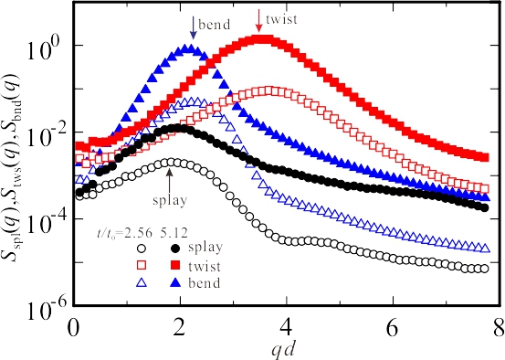
Figure 1: (color online) Decomposed structure factors of the nematic order parameter in isotropic-nematic phase transitions at $t=2.56t_{0}$ (empty symbols) and $5.12t_{0}$ (full symbols). Black circles, red squares, and blue triangles represent the splay, Twist, and bend modes, respectively. Peak positions predicted by the linearized analysis are marked by the arrows.

The linearized analysis indicates that the fluctuation of $\phi$ and the splay mode are coupled to each other. However, our simulated structure factor $\phi$ does not show an appreciable peak (data not shown). We consider that this is an artifact of our numerical simulation, because the complex spatial operators in the kinetic equations are difficult to deal with precisely. We need to improve the numerical scheme to study the spatial distribution of $\phi$ more quantitatively.

III.2 Growth of polydomain for $L_{\rm r}=0$

Next, we study the temporal evolution of the polydomain pattern in 3D. We set $\alpha=16v_{0}$, $\Delta x=d$, and $\Delta t=0.05t_{0}$. The initial condition is $\bar{\phi}=0.5$, which is larger than $\phi_{2}$, and $\bar{Q}_{ij}=0$ with the random noise. Figure 2(a) shows the temporal evolution of the pattern of $Q_{xy}^{2}$ in an $xy$-plane ($z=0$). The corresponding director field at $t=8000t_{0}$ in the same $xy$-plane is shown in Fig. 2(b). A polydomain pattern is formed and it coarsens in time. Figure 3 schematically explains how the isotropic-nematic transition takes place without molecular rotation. If the rotational motion is allowed, the rodlike polymers rotate to align with fixed positions as shown in Fig. 3(a). On the other hand, when the rotational motion is severely suppressed, the rodlike polymers that are initially nearly parallel to each other assemble to form a small grain via diffusion along their axes. The assembled grains form a mosaic pattern and many defects remain as shown in Fig. 3(b). In the latter case, the nematic order parameter is conserved in the whole system.

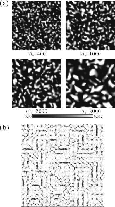
Figure 2: (a) Snapshots of $Q_{xy}^{2}$ in an $xy$ plane ($z=0$) at $t/t_{0}=400,\,1000,\,2000$, and $8000$ in the isotropic-nematic transition without rotational diffusion. (b) The corresponding director field of the domain pattern in the same $xy$ plane at $t=8000t_{0}$. The lines represent the principle axes of the tensorial order parameters.

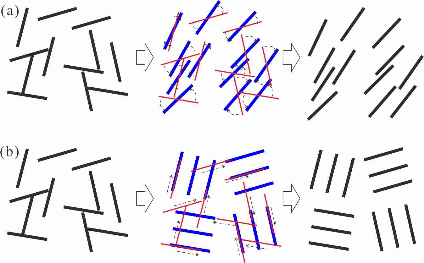
Figure 3: (color online) Process of isotropic-nematic transition in a solution of rodlike polymers. (a) When the rotational motion is allowed, the polymers rotate to align with fixed positions as in LMWLCs. (b) In the absence of rotational motion, the rodlike molecules diffuse only along their rod direction to form small grains of the nematic phase. In the center column, red and blue segments represent initial (left) and ordered (right) configurations, respectively. Arrows of broken lines indicate the motions of the rodlike polymers.

The defects in Fig. 2 are at the intersections of disclination lines in the $xy$-plane ($z=0$), entangled in three dimensions. In 2D Schlieren textures, the number of bright brushes forming a defect core is given by $4|m|$, where $m$ is the topological strength of the defect. We observed that most defects have two brushes in Fig. 2(a). As in other nematic states of LMWLCs, disclination lines of $m=\pm 1/2$ are formed more frequently than other types of defects.

Since the molecular rotation is severely suppressed in LCPs, its coarsening mechanism is very different from that in LMWLCs. Even after the early stage, the scalar nematic order parameter, which is given by $Q^{0}=(2Q_{ij}Q_{ji}/3)^{1/2}$, remains inhomogeneous; usually, $Q^{0}$ is smaller than the equilibrium nematic order $Q^{\rm eq}$ near the defects. Since the inhomogeneity of $Q^{0}$ affects the structure factor in the high $q$-range, we calculate the structure factor of a normalized order parameter, $\hat{Q}_{ij}=Q_{ij}/Q^{0}$, to determine the evolution of the polydomain pattern. This normalization corresponds to a binarization method for phase separation Shinozaki1993 .

In Fig. 4(a), we plot the temporal change of the total structure factor $S_{\rm tot}(q)=|\tilde{Q}_{ij}(\mbox{\boldmath$q$})|^{2}$, in which $\tilde{Q}_{ij}(\mbox{\boldmath$q$})$ refers to the Fourier transform of $\hat{Q}_{ij}(\mbox{\boldmath$r$})$. The structure factor is not decomposed into the three modes given by Eqs. (20)-(22). It is shown that the peak position of the structure factor shifts toward $q=0$ and the peak height develops with time. These features are similar to those in the late stage of phase separation Onukibook ; Shinozaki1993 . It is known that the structure factor scaled by the characteristic wave number collapses into a master curve at isotropic phase separation. We replot the scaled structure factor, $\hat{S}_{\rm tot}(q)=\langle{q(t)}\rangle^{3}S_{\rm tot}(q/\langle{q(t)}\rangle)$, in Fig. 4(b) and the characteristic wave number is defined as

$$\langle{q(t)}\rangle=\frac{\int d\mbox{\boldmath$q$}S(\mbox{\boldmath$q$},t)_{\rm tot}|\mbox{\boldmath$q$}|}{\int d\mbox{\boldmath$q$}S_{\rm tot}(\mbox{\boldmath$q$},t)}.$$ (23)

Figure 4(b) shows that the dynamic scaling law holds fairly well in the isotropic-nematic transition of rodlike polymers.

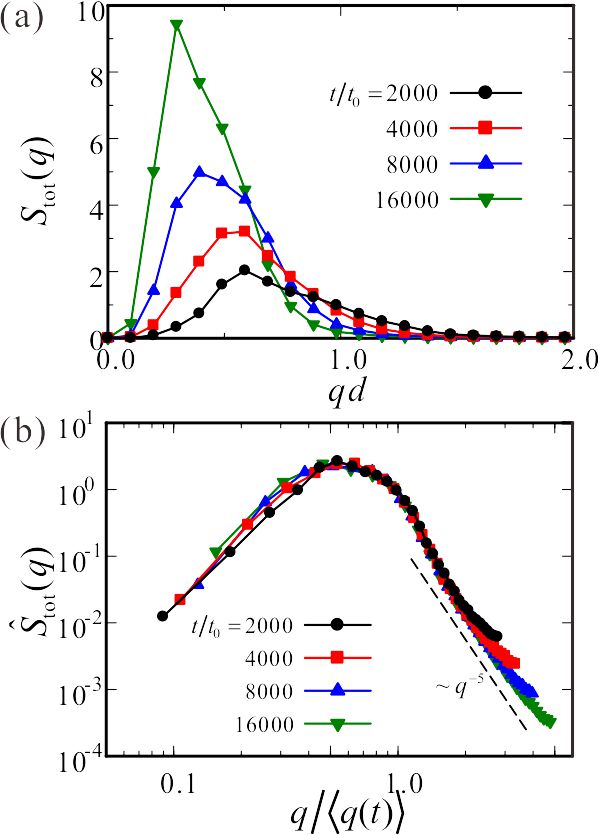
Figure 4: (color online) (a) Temporal changes in the total structure factor of the nematic order parameter in isotropic-nematic transitions without rotational diffusion. (b) Structure factor $\hat{S}_{\rm tot}(q)$ scaled by the characteristic wave number $\langle{q(t)}\rangle$ of the domain pattern. $\hat{S}_{\rm tot}(q)$ shows the domain growth with self similarity and the Porod law $\hat{S}_{\rm tot}\sim q^{-5}$ is observed in the high $q$-regime.

In the high wave number range ($q>\langle{q(t)}\rangle)$, the structure factor decays as $\tilde{S}_{\rm tot}(q)\sim q^{-5}$. In phase separation, a decay $S(q)\sim q^{-4}$, termed as Porod’s law, which originates from the scattering of 2D interfaces in a 3D matrix, has been observed Onukibook .

The $q^{-4}$-tail was also reported in 2D simulations of a nematic phase Zapotocky1995 ; Denniston2001 . The $q^{-5}$-tail observed in LCPs is considerably different from these tails. In similar systems, Bray studied phase transitions described by a conserved $N$-vector order parameter Bray1990 , and showed that the structure factor exhibited a $q^{-(N+3)}$-tail in 3D. From his work, it follows that a $q^{-5}$-tail is obtained for a system of $N=2$ or $XY$ model, in which many line defects are formed. We consider that the $q^{-5}$-tail observed in LCPs represents scattering from the entangled one dimensional (1D) disclination lines in the 3D matrix.

The self-similarity in the scaled structure factors indicates that the polydomain growth is characterized by only one characteristic length scale. We plot the temporal change of the characteristic polydomain size, which is defined as $\ell(t)=2\pi/\langle{q(t)}\rangle$ in Fig. 5. After the early stage, the characteristic size develops with time as $\ell(t)\sim t^{\alpha}$ with $\alpha=1/4$. This exponent is smaller than those in phase separation ($\alpha=1/3$) and isotropic-nematic transition of LMWLCs ($\alpha=1/2$) Toyoki1994 ; Fukuda1998 ; Denniston2001 . Interestingly, the exponent is the same as that of a system described by a conserved $XY$ model Bray1990 ; Siegert1993 . This coincidence and the same Porod’s tail value imply profound similarities between LCPs and the conserved $XY$ model. Therefore, the analysis of the conserved $XY$ model might be helpful to understand the coarsening mechanism in LCPs. However, there is also an important difference between the two; while most defects have $m=\pm 1/2$ topological strengths in the nematic state of rodlike polymers, the topological strengths in the $XY$ model are $m=\pm 1$. Further studies are needed to clarify the similarities and differences between them.

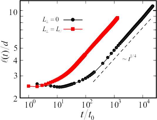
Figure 5: (color online) Time evolutions of the characteristic domain length $\ell(t)$. Black and red symbols represent those for $L_{\perp}=0$ and $L_{\perp}=L_{\parallel}$, respectively. Rotational diffusion is set to $L_{\rm r}=0$. In both the cases, characteristic lengths grow with time according to $\ell(t)\sim t^{1/4}$.

We have also studied the effect of the perpendicular diffusion on the polydomain growth. We set $L_{\perp}=L_{\parallel}$ and $L_{\rm r}=0$, where the off-diagonal terms of the kinetic equations (17) and (18) vanish. Since the rotational diffusion is not included, the tensorial order parameter $Q_{ij}$ is still conserved. The numerical simulations show that the dynamic scaling law holds and the growth exponent is also given by $\alpha=1/4$ as shown in Fig. 5 (red squares). It is indicated that this growth exponent is not characteristic of the parallel diffusion, but stems from the nature of the preserved order parameter. The characteristic length for $L_{\perp}=L_{\parallel}$ grows faster with time than for $L_{\perp}=0$ by a factor of approximately 1.6.

III.3 Growth of polydomain for $L_{\rm r}>0$

Solutions of LCPs have a very small but finite rotational diffusion coefficient $D_{\rm r}$. Thus, we expect that the polydomain growth will be affected by the rotational diffusion in the late stage of phase ordering. Figure 6 shows the temporal change of the scaled structure factor, $\hat{S}_{\rm tot}(q)$. Here, we set $L_{\perp}=0$ and $L_{\rm r}d^{2}/L_{\parallel}=0.0625$ and the other parameters are the same as those for $L_{\rm r}=L_{\perp}=0$. In the early stage, the structure factor has the same features as those in Fig. 4, namely, $\hat{S}_{\rm tot}(q)$ is very small at $q\sim 0$ and it has a peak at an intermediate wave number. With time, the structure factor in the lower $q$-range develops and in the late stage, $\hat{S}_{\rm tot}(q)$ has the Ornstein-Zernike form $S(q)\sim(1+q^{2}\ell^{2})^{-1}$, which is also observed in LMWLCs. The dynamic scaling law does not hold during the whole phase transition process and the growth of $\hat{S}_{\rm tot}(q)$ in the lower $q$-range is attributed to the rotational motion of rodlike polymers.

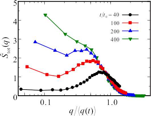
Figure 6: (color online) Time development of the scaled structure factor, $\hat{S}_{\rm tot}(q)$, in the isotropic-nematic transition with rotational diffusion, $L_{\rm r}d^{2}=0.0625L_{\parallel}$. Gradual evolution in the low $q$-regime is observed after the crossover time $t_{\rm cr}\cong 100t_{0}$.

In Fig. 7, we show the time evolution of $\ell$ for a number of $L_{\rm r}$’s. Although the physical meaning of $\ell$, especially in the crossover period (see below), is not clear, it is still a useful measure for the pattern growth. In the early stage, it does not change with time. This steady length corresponds to the spinodal decomposition-like growth of the nematic order parameter. After the early stage, the domain length evolves obeying $\ell\sim t^{1/4}$ as in the case of $L_{\rm r}=0$. Figure 7 indicates that the growth exponent changes from $\alpha=1/4$ to $\alpha=1/2$, which is the same as in the case of phase transition of LMWLCs, during a crossover period. Fig. 7 also indicates that the crossover depends on the rotational diffusion constant. As $L_{\rm r}$ increases, the crossover is observed at earlier times.

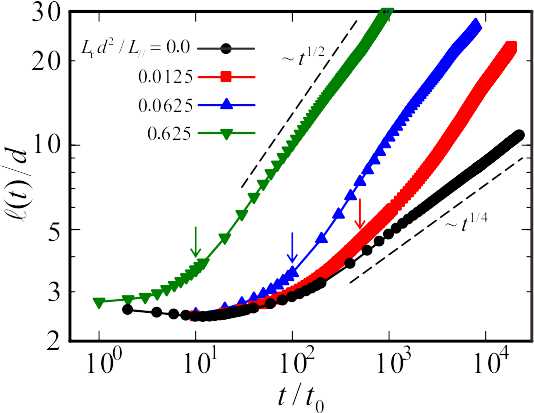
Figure 7: (color online) Temporal changes in the characteristic domain lengths in the isotropic-nematic transitions in LCPs. Rotational diffusion constant is varied as $L_{\rm r}d^{2}/L_{\parallel}=0,\,0.0125,\,0.0625$, and $0.625$. The occurrence of crossovers is indicated by arrows , and their positions are given by $t_{\rm r}=6.25/D_{\rm r}$.

Each rodlike polymer moves along a tube surrounded by other tubes. The tubes are not necessarily straight and they disappear in a certain period of time, New tubes are continually created as the surrounding molecules fluctuate. As a result, the polymer gradually loses its original orientation Doi1984 . We estimate that the crossover time $t_{\rm cr}$ is of the order of the characteristic rotational time $D_{\rm r}^{-1}$. After the crossover, the orientational order parameter is no longer conserved. In Fig. 7, arrows mark the corresponding crossover times and we assume $t_{\rm cr}=6.25t_{0}L_{\parallel}/(L_{\rm r}d^{2})$. Although it is difficult to determine exactly when the exponent changes from $\alpha=1/4$ to $\alpha=1/2$, the values marked by the arrows appear to be consistent with this interpretation.

In Fig. 8, we show the time evolution of the Schlieren pattern $Q_{xy}^{2}$ in an $xy$-plane for $L_{\rm r}d^{2}/L_{\parallel}=0.625$ and the crossover time is estimated as $t_{\rm cr}\cong 10t_{0}$. In an LCP solution with a finite $L_{\rm r}$, the director field rotates slowly, but freely, to adjust to the surrounding molecules.

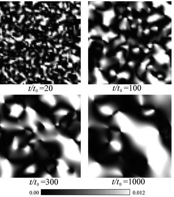
Figure 8: Snapshots of $Q_{xy}^{2}$ in the $xy$ plane after the crossover. Rotational diffusion constant is $L_{\rm r}d^{2}=0.625L_{\perp}$.

III.4 Defect motion

We study the finite-size effects on the stability of defects, mediated by the elastic field of the nematic phase for a defect pair of anti-signed topological charges. As there is an attractive interaction between the charges, the defects approach and annihilate each other. It was reported that the separation of $R$ between the defects decreases to zero with time as $R\sim(t_{\rm a}-t)^{\beta}$ with $\beta=1/2$, where $t_{\rm a}$ is the annihilation time Zapotocky1995 ; Toth2002 ; Svensek2002 . After annihilation, the director field relaxes to a homogeneous state in order to release the elastic energy in LMWLCs. However, this argument is not applicable to LCPs, since the kinetic mechanism is different.

In the simulations, $\alpha=16v_{0}$, $\bar{\phi}=0.5$, $\Delta x=0.2d$, and $\Delta t=0.0002t_{0}$, and we set $L_{\perp}=0$ and $L_{\rm r}=0$ to consider only parallel diffusions, i.e., those along the polymer molecular axis. We place a pair of anti-signed defects ($m=\pm 1/2$) in a small square box and carry out 2D simulations to mimic two parallel disclination lines with topological strengths of $m=\pm 1/2$.

Initially, the spatial distribution of $Q_{ij}$ is set to $Q_{ij}=3Q^{\rm eq}\left(u_{i}u_{j}-\delta_{ij}/3\right)/2$ with

$$\mbox{\boldmath$u$}(\mbox{\boldmath$r$})=(\cos\{(\theta_{+}-\theta_{-})/2\},\sin\{(\theta_{+}-\theta_{-})/2\},0).$$ (24)

Here, $\theta_{+}(\mbox{\boldmath$r$})$ is the angle between $(\mbox{\boldmath$r$}-\mbox{\boldmath$r$}_{+})$ and $(\mbox{\boldmath$r$}_{-}-\mbox{\boldmath$r$}_{+})$, and vice versa. $\mbox{\boldmath$r$}_{+}$ and $\mbox{\boldmath$r$}_{-}$ are the defect positions of $m=1/2$ and $m=-1/2$, respectively Toth2002 . At $t=0$, $(\mbox{\boldmath$r$}_{+}+\mbox{\boldmath$r$}_{-})/2$ is at the center of the box and $\mbox{\boldmath$r$}_{+}-\mbox{\boldmath$r$}_{-}$ is along the $x$-axis. This configuration is not the equilibrium structure of the defect positions, because the spatial variations of the scalar nematic order parameter and the non-linear terms are neglected. The absence of these terms do not affect our results, since the structure relaxes quickly before defect motions are excited. In order to avoid numerical artifacts near the boundary wall, we employ the periodic boundary condition; this may be inappropriate to study the realistic confinement effects on the defect motion; however, as there are only two defects in the system, the simulations give valuable insights into the stability of the defects.

Figure 9 shows time evolution of the director fields in $Q_{ij}$. In Fig. 9(a), the initial defect separation is $R(0)=|\mbox{\boldmath$r$}_{+}-\mbox{\boldmath$r$}_{-}|=12\Delta x$ and the box is $H^{2}$, where $H=48\Delta x$. The two defects approach and annihilate each other at $t\cong 153.3t_{0}$. Contrary to the cases in LMWLCs, the director field remains distorted even after a long annealing time. This is because the $y$-component of the director field is preserved. In other words, the rodlike polymers, which are initially oriented along the $y$-axis, remain permanently aligned with the axis if $L_{\rm r}=0$.

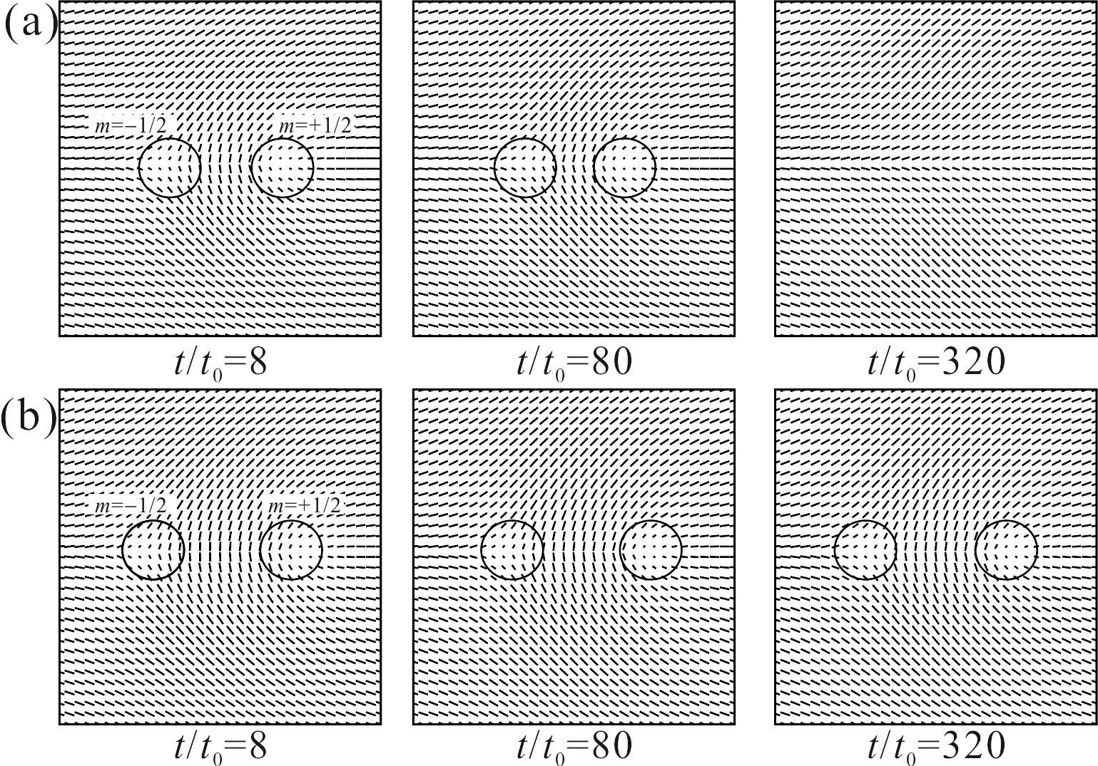
Figure 9: Director fields around a pair of anti-signed defects at $t/t_{0}=8$, $80$, and $320$. The initial separation between the defects is (a) $R(0)=12\Delta x$ and (b) $R(0)=16\Delta x$. The square box size is $H=48\Delta x$ and rotational diffusion is not allowed. Owing to the conservation of the order parameter, the director field remains deformed even after the defects are annihilated. At large separations, the defect structure is stabilized.

The free energy of the final distorted state in Fig. 9(a) is lower than that of a uniform nematic state with the same average order parameter $\bar{Q}_{ij}$. Here, it is important that $\bar{Q}_{ij}$ differs from the equilibrium value $Q^{\rm eq}_{ij}$. The final distorted state is determined by the balance between the local and non-local terms in the free-energy functional [Eqs. (10) and (12)]. For LMWLCs, the director field in the equilibrium state can optimize both parts of the free energy, such that $\bar{Q}_{ij}=Q^{\rm eq}_{ij}$. On the other hand, as the lowering of the local part has to induce the deformation of the director field in LCPs, it is reasonable to assume that the elastic distortion remains even in the final state.

Figure 10 plots the free energy at $t=800t_{0}$ calculated by Eqs. (10) and (12) versus the initial separation in a square box of $H=32\Delta x$. With increasing $R(0)$, the free energy is increased for $R(0)\lesssim 11\Delta x$. This increase enhances the elastic distortion without the formation of defects, as observed in Fig. 9. A kink in the free energy is observed around $R\cong 11.5\Delta x$. In Fig. 10, the free-energy difference from a reference $\{\mathcal{F}(11\Delta x)+\mathcal{F}(12\Delta x)\}/2$ is plotted. This kink represents the critical separation $R_{\rm t}$, above which the defects do not annihilate each other and remain even after a long annealing time ($t=800t_{0}$). The snapshots of the stabilized director field for $R(0)=16\Delta x$ in the box of $H=48\Delta x$, are shown in Fig. 9(b). These stable defects also stem from the conservation of the order parameter. As the initial separation increases, the amount of the rodlike polymers oriented along the $y$-axis increases, so that the elastic field is appreciably distorted. Above the critical separation, the formation of local singular points (defects) are preferable to gradual distortion without defects.

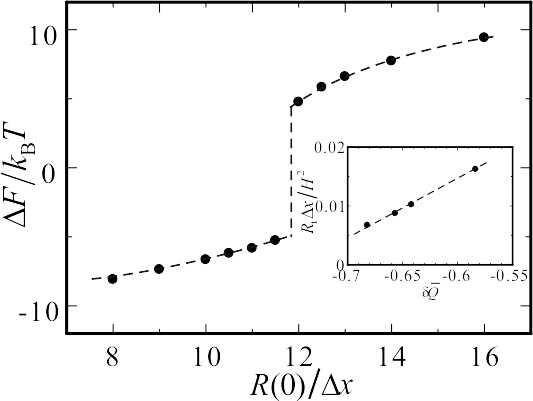
Figure 10: Plot of the free-energy difference at $t=800t_{0}$ with respect to the initial separation of the defect pair. The box size is fixed at $H=32\Delta x$ and the jump around $R(0)\cong 11.5\Delta x$ represents the threshold $R_{\rm t}$, above which defects remain even after a long annealing time. Inset: reduced threshold $R_{\rm t}\Delta x/H^{2}$ vs. $\delta\bar{Q}$.

The critical separation depends on the system size. Figure 11(a) shows the defect positions as a function of time. We fix the initial separation to $R=12\Delta x$ and vary the system size by $H/\Delta x=32$, $48$, and $64$. In the largest system, the defects approach faster and as $H$ decreases, the defect motion becomes slower and the resultant annihilation time is retarded. For $H=32\Delta x$, the defects initially experience a small shift at early times ($t\lesssim 10t_{0}$) and then hardly move. This dependence on the system size is unique to LCPs, and is not observed in LMWLCs. When the system size is large, there is a lot of room for the incompatible rodlike polymers to diffuse. In the inset of Fig.10, we show the dependence of the threshold $R_{\rm t}$, on the average order parameter difference, $\delta\bar{Q}=\int d\mbox{\boldmath$r$}(Q_{yy}-Q_{xx})/H^{2}$. In the initial configuration, the rodlike polymers along the $y$-axis are localized in between the two defects; therefore, the total amount of polymers is expected to be proportional to the defect separation, i.e.,, $\int d\mbox{\boldmath$r$}(Q_{yy}-Q_{xx})\propto R$. When $|\delta\bar{Q}|$ is smaller than a critical value, the solution cannot relax to a homogeneous nematic phase without defects and the simple scaling relation for the critical defect separation is $R_{\rm t}/H^{2}\propto\delta\bar{Q}$.

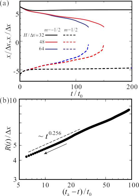
Figure 11: (color online) (a) Time evolutions of the positions to the right ($m=1/2$) and left ($m=-1/2$). Initial separation is $R(0)=12\Delta x$ and the box size is varied as $H/\Delta x=32,\,48$, and $64$. When $H=32\Delta x$, the defect positions are almost fixed after a small shift in the early stage. (b) Separation of the defect pair as a function of $t_{\rm a}-t$, where $t_{\rm a}$ is the annihilation time. Initial separation and the box size are $R(0)=12\Delta x$ and $H=48\Delta x$, respectively. The curve is fitted with the function $(t_{\rm a}-t)^{\beta}$, where $t_{\rm a}=153.3t_{0}$ and $\beta=0.256$.

This size dependence is similar to that in systems described by a single scalar order parameter. Here, we consider a system whose free energy has two minima below its critical point. We assume that a droplet of one phase is placed in a matrix of the other phase and if the order parameter is not conserved, the droplet will be adsorbed in the matrix phase, as in magnetism. When the order parameter is conserved, as in phase separation, the droplet can stably exist in a confined system. In its steady state, the radius of the droplet is determined by the average volume fraction of the components, and the concentration of the matrix phase is slightly supersaturated compared to the equilibrium concentration. This supersaturation is related to the interface tension given by the Gibbs-Duhem relationship Onukibook . As the volume of the confined box increases with a fixed droplet radius, the droplet evaporates and the system becomes homogeneous. This is because supersaturation decreases with increasing box size and the resultant critical droplet size is increased. In LMWLCs, the supersaturation relaxes locally and quickly to the equilibrium state. On the other hand, in LCPs, the system is “supersaturated” from the equilibrium state and the large supersaturation leads to the deformation of the director field.

In Fig. 11(b), we replot the defect separation as a function of reduced time, $t_{\rm a}-t$. The initial separation is $R=12\Delta x$ in a square box of $H=48\Delta x$, and the defects annihilate each other at $t=t_{\rm a}(\cong 153.3t_{0})$. We estimate the exponent $\beta\cong 0.256$ in $R\sim(t_{\rm a}-t)^{\beta}$ by fitting the curve. This is considerably smaller than $\beta=0.5$ for LMWLCs and close to the growth exponent $\alpha$. Note that the annihilation exponent $\beta$ is also of the same value as the growth exponent $\alpha$ in LMWLCs; however, the mechanism is not clearly understood and we have not concluded whether this exponent is universal for LCPs. Interestingly, Fig. 11(a) also suggests that the defect motion before the annihilation becomes asymmetric; the defect for $m=1/2$ moves faster than the defect for $m=-1/2$. Asymmetric motions of defects are also observed in LMWLCs with hydrodynamic interactions Toth2002 ; however, these interactions are absent in our model.

IV Conclusion

We studied the isotropic-nematic transition in liquid crystalline polymers by integrating the time-dependent Ginzburg-Landau equations for the compositional order parameter $\phi$ and the orientational order parameter $Q_{ij}$. The kinetic coefficients are evaluated using the Fokker-Planck equation Shimada1988c . This approach ensures that the rodlike polymers diffuse only in the direction parallel to their molecular axis.

Even if rotational motion is not allowed, the polymers being nearly parallel to each other assemble to form a nematic grain in the early stage of the phase transition. Since the director field is randomly oriented before the quenching of the isotopic phase, a polydomain structure is formed and many defects remain at the grain boundaries. The polydomain growth then exhibits self-similarity and the growth exponent is $\alpha=1/4$, which is considerably smaller than that for nematic liquid crystals of low molecular weight molecules. This small exponent is similar to those found in systems with conserved vector order parameters Bray1990 . Here, the structure factor of the nematic order parameter has a peak at an intermediate wave number and nearly vanishes at $q\sim 0$. Hence, the orientational order parameter is preserved, contrary to that in LMWLCs.

We have also shown that small but finite rotational diffusions can dominate the dynamics after a crossover time $t_{\rm cr}$. After the crossover, the growth exponent changes to $\alpha=1/2$, which is same as that for LMWLCs, and the polydomain pattern and the structure factor are also similar to those of LMWLCs. We estimated the crossover time as $t_{\rm cr}\cong 1/D_{\rm r}$, which enables rodlike polymers to rotate and the system behaves as a normal nematic liquid crystal, as in LMWLCs. This estimation qualitatively explains our numerical results.

We have also shown that defect motion is strongly influenced by the conservation of the nematic order parameter. In LCPs, the defects can be stabilized in a confined system and the stability depends on the box size. When the stability is lowered by increasing the box size, a pair of anti-symmetric defects annihilate each other. The director field is distorted after the annihilation of the defect pair and the defect annihilation obeys the power law, i.e., $R\sim(t_{\rm a}-t)^{\beta}$ with $\beta\cong 0.25$.

There are many experimental studies on the phase transition of LCPs. However, most have been analyzed with the same kinetic equation used for LMWLCs. Before the crossover is reached, the molecule diffuses by a crossover length $\ell_{\rm cr}=(D_{\parallel}/D_{\rm r})^{1/2}$. For a semi-dilute solution of rodlike polymers, the crossover length $\ell_{\rm cr}$ is comparable to the molecular length $d$. In order to examine the crossover in the phase transitions in LCPs, one must carefully probe the structure factor around $q\sim 2\pi/d$ at very early times. In a concentrated solution, the rotational diffusion constant is approximated by $D_{\rm r}=\beta D_{\rm r}^{0}(\bar{\phi}d^{2}/w^{2})^{-2}$, where $\beta$ is the numerical factor Doi1984 ; Teraoka1985 . Hence, the crossover length is increased with the average volume fraction $\bar{\phi}$ as $\ell_{\rm cr}\sim\bar{\phi}d^{3}/w^{2}$. In a melt of LCPs or a highly concentrated solution of rodlike polymers, the crossover might be experimentally accessible, and we hope that our numerical study will stimulate detailed experimental observations in these systems in the near future.

Appendix A Isotropic approximation

When we derive the free-energy functional (Eq. (12)) and kinetic equations [Eqs.(17) and (18)], we employ the isotropic average approximation Shimada1988c . The isotropic average of $A(\mbox{\boldmath$u$})$ is defined by

$$\langle{A}\rangle_{\mbox{\boldmath$u$}}=\frac{1}{4\pi}\int d\mbox{\boldmath$u$}A(\mbox{\boldmath$u$}).$$ (25)

Then, the following formulas are obtained:

$$\langle{u_{i}}\rangle_{\mbox{\boldmath$u$}}=\langle{u_{i}u_{j}u_{k}}\rangle_{\mbox{\boldmath$u$}}=0,$$ (26)

$$\langle{u_{i}u_{j}}\rangle_{\mbox{\boldmath$u$}}=\frac{1}{3}\delta_{ij},$$ (27)

$$\langle{u_{i}u_{j}u_{k}u_{l}}\rangle_{\mbox{\boldmath$u$}}=\frac{1}{15}(\delta_{ij}\delta_{kl}+\delta_{ik}\delta_{jl}+\delta_{il}\delta_{jk}).$$ (28)

Furthermore, we obtained

$$\langle{|\mbox{\boldmath$u$}\times\mbox{\boldmath$u$}^{\prime}|}\rangle_{\mbox{\boldmath$u$}^{\prime}}=\frac{\pi}{4},$$ (29)

$$\langle{|\mbox{\boldmath$u$}\times\mbox{\boldmath$u$}^{\prime}|u_{i}^{\prime}u_{j}^{\prime}}\rangle_{\mbox{\boldmath$u$}^{\prime}}=-\frac{\pi}{32}(u_{i}u_{j}-3\delta_{ij}).$$ (30)

In deriving Eq. (12), we need higher-order moments of $u$ such as $\langle{|\mbox{\boldmath$u$}\times\mbox{\boldmath$u$}^{\prime}|u_{i}^{\prime}u_{j}^{\prime}u_{k}^{\prime}u_{l}^{\prime}}\rangle_{\mbox{\boldmath$u$}}$, which are given in Ref Shimada1988c .

Appendix B Excluded volume interaction between rodlike polymers

In Eq. (3), $W(\mbox{\boldmath$r$},\mbox{\boldmath$u$};\mbox{\boldmath$r$}^{\prime},\mbox{\boldmath$u$}^{\prime})$ represents the excluded volume interaction potential between rodlike polymers $(\mbox{\boldmath$r$},\mbox{\boldmath$u$})$ and $(\mbox{\boldmath$r$}^{\prime},\mbox{\boldmath$u$}^{\prime})$. In Fourier $k$-space, it is expressed by Straley1973 ; Shimada1988b

$$\tilde{W}(\mbox{\boldmath$k$},\mbox{\boldmath$u$},\mbox{\boldmath$u$}^{\prime}) = \int d\mbox{\boldmath$r$}W(\mbox{\boldmath$r$},\mbox{\boldmath$u$},\mbox{\boldmath$0$},\mbox{\boldmath$u$}^{\prime})e^{i\mbox{\boldmath$k$}\cdot\mbox{\boldmath$r$}}$$ (31)

$$= 2\alpha\left|\mbox{\boldmath$u$}\times\mbox{\boldmath$u$}^{\prime}\right|\frac{\sin(\mbox{\boldmath$K$}\cdot\mbox{\boldmath$r$})}{\mbox{\boldmath$K$}\cdot\mbox{\boldmath$u$}}\frac{\sin(\mbox{\boldmath$K$}\cdot\mbox{\boldmath$u$}^{\prime})}{\mbox{\boldmath$K$}\cdot\mbox{\boldmath$u$}^{\prime}},$$

where $\alpha$ is the interaction parameter that is estimated as $wd^{2}$. $K$ is defined as $\mbox{\boldmath$k$}d/2$, and $d$ and $w$ are the length and width of the rodlike molecules, respectively. We expanded it up to the order of $k^{4}$ using the following expansion:

$$\frac{\sin(\mbox{\boldmath$K$}\cdot\mbox{\boldmath$u$})}{\mbox{\boldmath$K$}\cdot\mbox{\boldmath$u$}}=1-\frac{(\mbox{\boldmath$K$}\cdot\mbox{\boldmath$u$})^{2}}{6}+\frac{(\mbox{\boldmath$K$}\cdot\mbox{\boldmath$u$})^{4}}{120}+\cdots.$$ (32)

This approximation is allowed for $k\leq 1/d$.

Appendix C Linear analysis

Here, we derive the growth rates of the order parameters in the early stage of the isotropic-nematic transition. We assume $L_{\perp}=L_{\rm r}d^{2}=0$ in the high concentration limit. The deviations of the order parameters from the initial conditions are so small that the chemical potential and molecular field are linearized as

$$\mu \cong \left(\frac{1}{\bar{\phi}}+\chi+C_{0}\mbox{\boldmath$q$}^{2}+C_{1}\mbox{\boldmath$q$}^{4}\right)\delta\phi+K_{0}q_{i}q_{j}\delta Q_{ij},$$ (33)

$$H_{ij} \cong \left(\frac{a_{0}}{\bar{\phi}}-a_{1}\right)\delta Q_{ij}+K_{0}q_{i}q_{j}\delta\phi+K_{1}\mbox{\boldmath$q$}^{2}\delta Q_{ij}+\frac{1}{2}K_{2}\left(q_{i}q_{k}\delta Q_{kj}+q_{j}q_{k}\delta Q_{ki}\right),$$ (34)

where $\delta\phi=\phi-\bar{\phi}$ and $\delta Q_{ij}=Q_{ij}$.

As noted in the main text, the orientational order parameter can be decomposed into the three modes splay, twist, and bend. According to Shimada et al., the kinetic equations are also linearized as

$$\frac{\partial{}}{\partial{t}}\delta\tilde{\phi} = -\Gamma_{\phi,\phi}(q)\delta\tilde{\phi}-\Gamma_{\phi,{\rm s}}(q)\delta\tilde{Q}_{\rm spl}$$ (35)

$$\frac{\partial{}}{\partial{t}}\delta\tilde{Q}_{\rm spl} = -\Gamma_{{\rm s},\phi}(q)\delta\tilde{\phi}-\Gamma_{\rm s,s}(q)\delta\tilde{Q}_{\rm spl}$$ (36)

$$\frac{\partial{}}{\partial{t}}\delta\tilde{Q}_{\rm tws} = -\Gamma_{\rm t,t}(q)\delta\tilde{Q}_{\rm tws},$$ (37)

$$\frac{\partial{}}{\partial{t}}\delta\tilde{Q}_{\rm bnd} = -\Gamma_{\rm b,b}(q)\delta\tilde{Q}_{\rm bnd},$$ (38)

where $\delta\tilde{Q}_{\rm spl}$, $\delta\tilde{Q}_{\rm tws}$, and $\delta\tilde{Q}_{\rm bnd}$ are the decomposed splay, twist, and bend modes of the tensorial order parameter $Q_{ij}$ in Fourier space, respectively. The decomposed structure factors in Sec. III.1 are obtained from them. For example, $\delta\tilde{Q}_{\rm spl}$ stands for $a_{i}\tilde{Q}_{ij}a_{j}$ in Eq. (20). The coefficients are given by

$$\Gamma_{\phi,\phi}(q) = \frac{1}{3}L_{\parallel}q^{2}\left\{A+\left(C_{0}+\frac{2}{5}K_{0}\right)q^{2}+C_{1}q^{4}\right\},$$ (39)

$$\Gamma_{\phi,{\rm s}}(q) = \frac{2}{15}L_{\parallel}q^{2}\left\{B+\left(\frac{5}{2}K_{0}+K_{1}+K_{2}\right)q^{2}\right\},$$ (40)

$$\Gamma_{{\rm s},\phi}(q) = \frac{4}{45}L_{\parallel}q^{2}\left\{A+\left(C_{0}+\frac{11}{14}K_{0}\right)q^{2}+C_{1}q^{4}\right\},$$ (41)

$$\Gamma_{\rm s,s}(q) = \frac{22}{415}L_{\parallel}q^{2}\left\{B+\left(\frac{14}{11}K_{0}+K_{1}+K_{2}\right)q^{2}\right\},$$ (42)

$$\Gamma_{\rm t,t}(q) = \frac{2}{35}L_{\parallel}q^{2}\left\{B+\left(K_{0}+\frac{1}{2}K_{1}\right)q^{2}\right\}$$ (43)

$$\Gamma_{\rm b,b}(q) = \frac{2}{105}L_{\parallel}q^{2}(B+K_{1}q^{2}),$$ (44)

where $A=\chi+1/\bar{\phi}$ and $B=a_{0}/\bar{\phi}-a_{1}$. Although $\Gamma_{\phi,\phi}$ and $\Gamma_{{\rm s},\phi}$ contain a negative $C_{0}$, both the growth rates increase monotonically with increasing $q$; therefore, a modulated pattern due to negative $C_{0}$ will not appear.

In the early stage, the concentration field and splay mode are coupled to each other via the off-diagonal terms. The eigenvalues of the coupled growth rates are $\Gamma_{\pm}=(\Gamma_{\phi,\phi}+\Gamma_{\rm s,s}\pm\sqrt{(\Gamma_{\phi,\phi}-\Gamma_{\rm s,s})^{2}+4\Gamma_{{\rm s},\phi}\Gamma_{\phi,{\rm s}}})/2$. The peak positions indicated in Fig. 1 are calculated by solving $d\Gamma_{X}(q)/dq=0$, where $\Gamma_{X}(q)$ represents $\Gamma_{+}(q)\,,\Gamma_{\rm t,t}(q)$, and $\Gamma_{\rm b,b}(q)$.

Shimada et al. derived similar dynamic equations for spinodal decomposition in an LCP solution Shimada1988c with the same initial equations; however, they derived their equations by expanding the Fokker-Planck equation directly and we obtain the free-energy functional and dynamic equations separately. However, it is noted that these differences are insignificant in the essential features of our results.