Renormalization group evolution of collinear and infrared divergences

Nikolaos Kidonakis
Kennesaw State University, Physics #1202, Kennesaw, GA 30144, USA

Abstract

I discuss collinear and infrared divergences in QCD cross sections with massless and massive final-state particles. I present the two-loop renormalization group evolution and resummation in terms of anomalous dimensions, and I show specific results for a variety of QCD hard-scattering processes.

RESUMMATION OF COLLINEAR AND SOFT CORRECTIONS

Soft-gluon corrections arise in scattering cross sections from incomplete cancellations of infrared divergences in virtual diagrams and real diagrams with low-energy (soft) gluons. At $n$th order in the perturbative series, these soft corrections are of the form $[(\ln^{k}(s_{4}/M^{2}))/s_{4}]_{+}$ with $M$ a hard scale, $k\leq 2n-1$ and $s_{4}$ the kinematical distance from threshold. The leading (double) logarithms arise from collinear and soft radiation. Also purely collinear terms $(1/M^{2})\ln^{k}(s_{4}/M^{2})$ appear in the cross section.

Soft-gluon corrections are dominant near threshold and they can be shown to exponentiate, so these corrections can be resummed. Resummation follows from factorization properties of the cross section and renormalization group evolution (RGE) [1, 2] (for further recent studies see Refs. [3-14]). At next-to-leading-logarithm (NLL) accuracy this requires one-loop calculations in the eikonal approximation. Recently results have been derived at next-to-NLL (NNLL), with the completion of two-loop calculations for soft anomalous dimensions for processes with massless and massive partons in various approaches [3,6-14]. Approximate NNLO and higher-order cross sections have also been derived from the expansion of the resummed cross sections.

The cross section factorizes as $\sigma=(\prod\psi)\;H_{IL}\,S_{LI}\;(\prod J)$, where $\psi$ are functions for the incoming partons, $J$ are final-state jet functions, $H$ is the hard-scattering function, and $S$ is the soft-gluon function describing noncollinear soft-gluon emission [2]. We use RGE to evolve the $S$ function associated with soft-gluon emission

$$\left(\mu{\partial\over\partial\mu}+\beta(g_{s}){\partial\over\partial g_{s}}\right)\,S_{LI}=-(\Gamma^{\dagger}_{S})_{LB}S_{BI}-S_{LA}(\Gamma_{S})_{AI}$$

where $\Gamma_{S}$ is the soft anomalous dimension, a matrix in color space and a function of the kinematical invariants of the process [2].

Solving the RGE for the soft function and the other functions in the factorized cross section, we find the following result for the resummed cross section in Mellin moment space, with $N$ the moment variable,

$${\hat{\sigma}}^{res}(N) = \exp\left[\sum_{i}E_{i}(N_{i})\right]\,\exp\left[\sum_{j}E^{\prime}_{j}(N^{\prime})\right]\;\exp\left[\sum_{i}2\int_{\mu_{F}}^{\sqrt{s}}\frac{d\mu}{\mu}\;\gamma_{i/i}\left({\tilde{N}}_{i},\mu\right)\right]\;$$

$$\times{\rm tr}\left\{H\exp\left[\int_{\sqrt{s}}^{{\sqrt{s}}/{\tilde{N}^{\prime}}}\frac{d\mu}{\mu}\Gamma_{S}^{\dagger}(\mu)\right]\;S(\sqrt{s}/\tilde{N}^{\prime})\exp\left[\int_{\sqrt{s}}^{{\sqrt{s}}/{\tilde{N}^{\prime}}}\frac{d\mu}{\mu}\Gamma_{S}(\mu)\right]\right\}\,.$$

Collinear and soft radiation from the incoming partons is resummed in the exponent

$$E_{i}(N_{i})=\int^{1}_{0}dz\frac{z^{N_{i}-1}-1}{1-z}\;\left\{\int_{1}^{(1-z)^{2}}\frac{d\lambda}{\lambda}A_{i}\left(\lambda s\right)+D_{i}\left[(1-z)^{2}s\right]\right\}.$$

Purely collinear terms can be derived by replacing $\frac{z^{N-1}-1}{1-z}\;$ by $\;-z^{N-1}$ above.

Collinear and soft radiation from outgoing massless quarks and gluons is resummed in the second exponent

$$E^{\prime}_{j}(N^{\prime})=\int^{1}_{0}dz\frac{z^{N^{\prime}-1}-1}{1-z}\left\{\int^{1-z}_{(1-z)^{2}}\frac{d\lambda}{\lambda}A_{i}\left(\lambda s\right)+B_{i}\left[(1-z)s\right]+D_{i}\left[(1-z)^{2}s\right]\right\}.$$

The quantities $A$, $B$, and $D$ have well-known perturbative expansions in $\alpha_{s}$. The factorization scale, $\mu_{F}$, dependence in the third exponent is controlled by parton anomalous dimensions $\gamma_{i/i}=-A_{i}\ln{\tilde{N}}_{i}+\gamma_{i}$. Noncollinear soft gluon emission is controlled by the process-dependent soft anomalous dimension $\Gamma_{S}$.

We determine $\Gamma_{S}$ from the coefficients of ultraviolet poles in dimensionally regularized eikonal diagrams [2,6,11-15]. We perform the calculations in momentum space and Feynman gauge. Complete two-loop results have been derived for the soft anomalous dimensions for $e^{+}e^{-}\rightarrow t{\bar{t}}$ [6], $t{\bar{t}}$ hadroproduction [13], $t$-channel [14] and $s$-channel [11] single top production, $tW^{-}$ and $tH^{-}$ production [12], and direct photon and $W$ production at large $Q_{T}$. We write the perturbative series for the soft anomalous dimension $\Gamma_{S}=(\alpha_{s}/\pi)\Gamma_{S}^{(1)}+(\alpha_{s}/\pi)^{2}\Gamma_{S}^{(2)}+\cdots$ and determine $\Gamma_{S}^{(1)}$ and $\Gamma_{S}^{(2)}$ for these processes.

TWO-LOOP SOFT ANOMALOUS DIMENSIONS

Top-antitop production in hadron colliders

The soft anomalous dimension matrix for the partonic process $q{\bar{q}}\rightarrow t{\bar{t}}$ is a $2\times 2$ matrix [2, 13]

$$\Gamma_{S\,q{\bar{q}}}=\left[\begin{array}[]{cc}\Gamma_{q{\bar{q}}\,11}&\Gamma_{q{\bar{q}}\,12}\\ \Gamma_{q{\bar{q}}\,21}&\Gamma_{q{\bar{q}}\,22}\end{array}\right].$$ (3)

At one loop, in a singlet-octet color basis, we find

$$\Gamma_{q{\bar{q}}\,11}^{(1)}=-C_{F}\,[L_{\beta}+1]\hskip 42.67912pt\Gamma_{q{\bar{q}}\,21}^{(1)}=2\ln\left(\frac{u_{1}}{t_{1}}\right)\hskip 42.67912pt\Gamma_{q{\bar{q}}\,12}^{(1)}=\frac{C_{F}}{C_{A}}\ln\left(\frac{u_{1}}{t_{1}}\right)$$

$$\Gamma_{q{\bar{q}}\,22}^{(1)}=C_{F}\left[4\ln\left(\frac{u_{1}}{t_{1}}\right)-L_{\beta}-1\right]+\frac{C_{A}}{2}\left[-3\ln\left(\frac{u_{1}}{t_{1}}\right)+\ln\left(\frac{t_{1}u_{1}}{sm^{2}}\right)+L_{\beta}\right]$$

where $L_{\beta}=[(1+\beta^{2})/(2\beta)]\ln[(1-\beta)/(1+\beta)]$ with $\beta=\sqrt{1-4m^{2}/s}$ and $m$ the top quark mass.

At two loops, we find [13]

$$\Gamma_{q{\bar{q}}\,11}^{(2)}=\frac{K}{2}\Gamma_{q{\bar{q}}\,11}^{(1)}+C_{F}C_{A}\,M_{\beta}\hskip 56.9055pt\Gamma_{q{\bar{q}}\,22}^{(2)}=\frac{K}{2}\Gamma_{q{\bar{q}}\,22}^{(1)}+C_{A}\left(C_{F}-\frac{C_{A}}{2}\right)\,M_{\beta}$$

$$\Gamma_{q{\bar{q}}\,21}^{(2)}=\frac{K}{2}\Gamma_{q{\bar{q}}\,21}^{(1)}+C_{A}N_{\beta}\ln\left(\frac{u_{1}}{t_{1}}\right)\hskip 42.67912pt\Gamma_{q{\bar{q}}\,12}^{(2)}=\frac{K}{2}\Gamma_{q{\bar{q}}\,12}^{(1)}-\frac{C_{F}}{2}N_{\beta}\ln\left(\frac{u_{1}}{t_{1}}\right)$$

where $K$ is a two-loop constant, $M_{\beta}$ is a part of the two-loop cusp anomalous dimension [6], and $N_{\beta}$ is a subset of the terms of $M_{\beta}$.

Similar results have been derived for the $gg\rightarrow t{\bar{t}}$ channel [13].

Single top quark production

We begin with the soft anomalous dimension for $t$-channel single top production [14]. Here we show results only for the 11 element of the matrix. At one loop

$${\Gamma}_{{\rm t\mbox{-}ch}\,11}^{(1)}=C_{F}\left[\ln\left(\frac{-t}{s}\right)+\ln\left(\frac{m^{2}-t}{m\sqrt{s}}\right)-\frac{1}{2}\right].$$

At two loops [14]

$$\Gamma_{{\rm t\mbox{-}ch}\,11}^{(2)}=\frac{K}{2}\Gamma_{{\rm t\mbox{-}ch}\,11}^{(1)}+C_{F}C_{A}\frac{(1-\zeta_{3})}{4}.$$

We continue with the soft anomalous dimension for $s$-channel single top production [11], again showing only the 11 matrix element:

$$\Gamma_{{\rm s\mbox{-}ch}\,11}^{(1)}=C_{F}\left[\ln\left(\frac{s-m^{2}}{m\sqrt{s}}\right)-\frac{1}{2}\right]\,,\quad\quad\Gamma_{{\rm s\mbox{-}ch}\,11}^{(2)}=\frac{K}{2}\Gamma_{{\rm s\mbox{-}ch}\,11}^{(1)}+C_{F}C_{A}\frac{(1-\zeta_{3})}{4}.$$

Finally we present the soft anomalous dimension for the associated production of a top quark with a $W^{-}$ or $H^{-}$. Relevant two-loop eikonal diagrams are shown in Fig. 1 (there are also additional top-quark self-energy graphs).

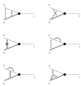
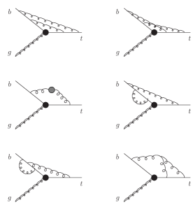
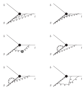
Figure 1: Two-loop eikonal diagrams for $tW$ production.

The soft anomalous dimension for $bg\rightarrow tW^{-}$ (or $bg\rightarrow tH^{-}$) is [12]

$$\Gamma_{S,\,tW^{-}}^{(1)}=C_{F}\left[\ln\left(\frac{m^{2}-t}{m\sqrt{s}}\right)-\frac{1}{2}\right]+\frac{C_{A}}{2}\ln\left(\frac{m^{2}-u}{m^{2}-t}\right)$$

$$\Gamma_{S,\,tW^{-}}^{(2)}=\frac{K}{2}\Gamma_{S,\,tW^{-}}^{(1)}+C_{F}C_{A}\frac{(1-\zeta_{3})}{4}\,.$$

$W$-boson and direct photon production at large $p_{T}$

One-loop results for the soft anomalous dimensions for $W$ (same as for direct photon) production have been known from [15]. Here we also present new two-loop results.

For the process $qg\rightarrow Wq$ (or $qg\rightarrow\gamma q$) the soft anomalous dimension is

$$\Gamma_{S,\,qg\rightarrow Wq}^{(1)}=C_{F}\ln\left(\frac{-u}{s}\right)+\frac{C_{A}}{2}\ln\left(\frac{t}{u}\right)\,,\quad\quad\Gamma_{S,\,qg\rightarrow Wq}^{(2)}=\frac{K}{2}\Gamma_{S,\,qg\rightarrow Wq}^{(1)}\,.$$

For the process $q{\bar{q}}\rightarrow Wg$ (or $q{\bar{q}}\rightarrow\gamma g$) the soft anomalous dimension is

$$\Gamma_{S,\,q{\bar{q}}\rightarrow Wg}^{(1)}=\frac{C_{A}}{2}\ln\left(\frac{tu}{s^{2}}\right)\,,\quad\quad\Gamma_{S,\,q{\bar{q}}\rightarrow Wg}^{(2)}=\frac{K}{2}\Gamma_{S,\,q{\bar{q}}\rightarrow Wg}^{(1)}\,.$$

ACKNOWLEDGMENTS

This work was supported by the National Science Foundation under Grant No. PHY 0855421.

References

• [1] H. Contopanagos, E. Laenen, and G. Sterman, Nucl. Phys. B 484, 303 (1997) [hep-ph/9604313].
• [2] N. Kidonakis and G. Sterman, Nucl. Phys. B 505, 321 (1997) [hep-ph/9705234].
• [3] S.M. Aybat, L.J. Dixon, and G. Sterman, Phys. Rev. D 74, 074004 (2006) [hep-ph/0607309].
• [4] L.J. Dixon, L. Magnea, and G. Sterman, JHEP 08, 022 (2008) [arXiv:0805.3515 [hep-ph]].
• [5] E. Gardi and L. Magnea, JHEP 03, 079 (2009) [arXiv:0901.1091 [hep-ph]].
• [6] N. Kidonakis, Phys. Rev. Lett. 102, 232003 (2009) [arXiv:0903.2561 [hep-ph]].
• [7] A. Mitov, G. Sterman, and I. Sung, Phys. Rev. D 79, 094015 (2009) [arXiv:0903.3241 [hep-ph]].
• [8] T. Becher and M. Neubert, Phys. Rev. D 79, 125004 (2009) [arXiv:0904.1021 [hep-ph]].
• [9] M. Beneke, P. Falgari, and C. Schwinn, Nucl. Phys. B 828, 69 (2010) [arXiv:0907.1443 [hep-ph]].
• [10] A. Ferroglia, M. Neubert, B. Pecjak, and L. Yang, JHEP 11, 062 (2009) [arXiv:0908.3676 [hep-ph]].
• [11] N. Kidonakis, Phys. Rev. D 81, 054028 (2010) [arXiv:1001.5034 [hep-ph]].
• [12] N. Kidonakis, Phys. Rev. D 82, 054018 (2010) [arXiv:1005.4451 [hep-ph]].
• [13] N. Kidonakis, Phys. Rev. D 82, 114030 (2010) [arXiv:1009.4935 [hep-ph]].
• [14] N. Kidonakis, Phys. Rev. D 83, 091503(R) (2011) [arXiv:1103.2792 [hep-ph]].
• [15] N. Kidonakis and V. Del Duca, Phys. Lett. B 480, 87 (2000) [hep-ph/9911460].