Exact diagonalization of the Bohr Hamiltonian for rotational nuclei: Dynamical $\gamma$ softness and triaxiality

Abstract

Detailed quantitative predictions are obtained for phonon and multiphonon excitations in well-deformed rotor nuclei within the geometric framework, by exact numerical diagonalization of the Bohr Hamiltonian in an $\mathrm{SO}(5)$ basis. Dynamical $\gamma$ deformation is found to significantly influence the predictions through its coupling to the rotational motion. Basic signatures for the onset of rigid triaxial deformation are also obtained.

I Introduction

The Bohr Hamiltonian bohr1952:vibcoupling ; bohr1998:v2 , together with its generalizations kumar1966:bohr-solution ; eisenberg1987:v1 , has long served as the conceptual benchmark for interpreting quadrupole collective dynamics in nuclei. The conventional approach to numerical diagonalization of the Bohr Hamiltonian, in a five-dimensional oscillator basis gneuss1969:gcm ; hess1980:gcm-details-238u ; eisenberg1987:v1 , is slowly convergent and requires a large number of basis states to describe a general deformed rotor-vibrator nucleus. Therefore, it has commonly been necessary to apply varying degrees of approximation in addressing the dynamics of transitional and deformed nuclei, as in the rotation-vibration model faessler1965:rvm and rigid triaxial rotor davydov1958:arm-intro treatments of the Bohr Hamiltonian, or in more recent studies of critical phenomena iachello2001:x5 ; iachello2003:y5 ; bonatsos2007:gamma-separable-x5 ; bonatsos2007:gamma-separable-davidson .

However, diagonalization of the Bohr Hamiltonian is now possible rowe2009:acm for potentials of essentially arbitrary stiffness. In particular, the algebraic collective model (ACM) rowe2004:tractable-collective ; rowe2005:algebraic-collective ; rowe2005:radial-me-su11 ; caprio2005:axialsep ; rowe2010:rowanwood provides an efficient and straightforward computational framework based on $\mathrm{SU}(1,1)\times\mathrm{SO}(5)$ algebraic methods. The Bohr Hamiltonian is diagonalized in a basis of $\mathrm{SU}(1,1)\times\mathrm{SO}(5)$ product wave functions on the Bohr deformation variables $\beta$ and $\gamma$ and Euler angles $\Omega$. These are of the form $R_{n}^{\lambda}(a;\beta)\Psi_{v\alpha LM}(\gamma,\Omega)$, where $R_{n}^{\lambda}$ is an $\mathrm{SU}(1,1)$ modified oscillator wave function rowe1998:davidson and $\Psi_{v\alpha LM}$ is an $\mathrm{SO}(5)\supset\mathrm{SO}(3)$ spherical harmonic rowe2004:spherical-harmonics ; caprio2009:gammaharmonic . The $\mathrm{SO}(5)\supset\mathrm{SO}(3)$ formulation may be used either simply to extend the conventional oscillator basis to higher phonon numbers sufficient to provide full convergence debaerdemacker2007:so5-cartan ; debaerdemacker2008:collective-cartan ; debaerdemacker2009:acm-spectra or, further, to obtain much faster convergence as a function of basis size through the use of $\mathrm{SU}(1,1)$ $\beta$ wave functions chosen optimally for the nuclear deformation rowe2005:algebraic-collective .

The Bohr Hamiltonian can consequently be applied, without approximation, to the full range of nuclear quadrupole rotational-vibrational structure, from spherical oscillator to axial rotor to triaxial rotor. Full convergence can be obtained for energies and electromagnetic transition strengths involving high-lying states, for instance, interband transitions among $\beta$, $\gamma$, and multiphonon bands in well-deformed rotor nuclei. The Bohr Hamiltonian inherently induces coupling of the $\beta$, $\gamma$, and rotational degrees of freedom, thereby yielding a rich set of phenomena.

To approach an understanding of the full problem, we shall consider, in this article, the simpler but already extensive implications of coupling of the $\gamma$ and rotational degrees of freedom. The relevant Hamiltonian is then the “angular” part of the Bohr Hamiltonian, and the ACM calculation reduces to diagonalization in a basis of $\mathrm{SO}(5)\supset\mathrm{SO}(3)$ spherical harmonics (Sec. II). The regime we address consists of rotational structure with axially symmetric (axial) or weakly triaxial deformation. However, even for a nominally axial rotor, the Bohr description is found to mandate significant dynamical fluctuations in $\gamma$, far from $\gamma=0^{\circ}$. The evolution of spectroscopic quantities (energies and transition matrix elements) with respect to the $\gamma$ confinement provided by the potential is systematically investigated (Sec. III), and the spectroscopic implications of the onset of rigid triaxial structure are explored (Sec. IV). Probability distributions with respect to $\gamma$ and with respect to the $K$ quantum number are then used to examine the degree of adiabaticity, or separation of rotational and vibrational degrees of freedom in the wave functions (Sec. V). Preliminary results were presented in Refs. caprio2008:acm-cgs13 ; caprio2009:gammatriax .

II Hamiltonian and solution method

II.1 Hamiltonian

The Bohr Hamiltonian bohr1998:v2 is given, in terms of the quadrupole deformation variables $\beta$ and $\gamma$ and Euler angles $\Omega$, by

$$H=-\frac{\hbar^{2}}{2B}\biggl{[}\frac{1}{\beta^{4}}\frac{\partial}{\partial\beta}\beta^{4}\frac{\partial}{\partial\beta}-\frac{\hat{\Lambda}^{2}}{\beta^{2}}\biggr{]}+V(\beta,\gamma),$$ (1)

where

$$\hat{\Lambda}^{2}=-\biggl{(}\frac{1}{\sin 3\gamma}\frac{\partial}{\partial\gamma}\sin 3\gamma\frac{\partial}{\partial\gamma}-\frac{1}{4}\sum_{\kappa}\frac{\hat{L}_{\kappa}^{\prime 2}}{\sin^{2}(\gamma-\frac{2}{3}\pi\kappa)}\biggr{)}.$$ (2)

The operator appearing in brackets in the kinetic energy is the Laplacian in five dimensions. Its angular part $\hat{\Lambda}^{2}$ is the Casimir operator for the five-dimensional rotation group $\mathrm{SO}(5)$, which contains the rotations in physical space, acting on the Euler angle coordinates, as an $\mathrm{SO}(3)$ subgroup. The Bohr coordinates are five-dimensional spherical polar coordinates, in terms of which the five components $q_{M}$ ($M=-2$, $\ldots$, $2$) of the quadrupole deformation tensor are expressed as

$$q_{M}=\beta\biggl{[}\cos\gamma\,\mathscr{D}^{(2)}_{0,M}(\Omega)\\ +\frac{1}{\sqrt{2}}\sin\gamma\bigl{[}\mathscr{D}^{(2)}_{2,M}(\Omega)+\mathscr{D}^{(2)}_{-2,M}(\Omega)\bigr{]}\biggr{]}.$$ (3)

The potential energy $V(\beta,\gamma)$ must be periodic in $\gamma$, with period $120^{\circ}$, and it must be symmetric about $\gamma=0^{\circ}$ and $\gamma=60^{\circ}$. The Bohr coordinate system and Hamiltonian are reviewed in detail in, e.g., Ref. prochniak2009:bohr-collective-hf-hg .

The restriction to angular coordinates $(\gamma,\Omega)$ then yields a Hamiltonian

$$H=\hat{\Lambda}^{2}+V(\gamma).$$ (4)

Such an angular Hamiltonian arises as a schematic limit of the full Bohr Hamiltonian when the coordinate $\beta$ in (1) is taken to be rigidly fixed, as might be considered for a well-deformed nucleus. However, a reduction to the angular form (4) is more broadly applicable to transitional nuclei as well bonatsos2007:gamma-separable-x5 ; bonatsos2007:gamma-separable-davidson , since it occurs by separation of variables when the potential is of the form $V(\beta,\gamma)=u(\beta)+v(\gamma)/\beta^{2}$ jean1960:transition-model . The explicit relations for reduction to an angular Hamiltonian are reviewed in Appendix A. The symmetry conditions on $V(\gamma)$ are satisfied by the function $\cos 3\gamma$ and powers $\cos^{n}3\gamma$ thereof.

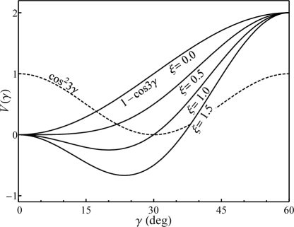
Figure 1: The shape of the potential $V(\gamma)$ used in (5), plotted for various values of $\xi$ (taking $\chi=1$). Note that a constant offset $\xi$ has been subtracted from each curve, so that $V(0)=0$ in each case. The dotted curve indicates the shape of the contribution from $\cos^{2}3\gamma$.

Let us therefore consider, in particular,

$$H=\hat{\Lambda}^{2}+\chi\bigl{[}(1-\cos 3\gamma)+\xi\cos^{2}3\gamma\bigr{]}.$$ (5)

The possible shapes of the potential appearing in this Hamiltonian are shown in Fig. 1. For $\xi=0$, $V(\gamma)\propto(1-\cos 3\gamma)$, as considered in Ref. rowe2004:tractable-collective , providing a minimum at $\gamma=0^{\circ}$ (axial deformation). With increasing $\chi$, a “deeper” potential provides greater confinement or stabilization around $\gamma=0^{\circ}$, approximately harmonic ($\propto\gamma^{2}$) for small $\gamma$. Including a $\cos^{2}3\gamma$ term [Fig. 1 (dotted curve)] by taking $\xi$ nonzero introduces a richer extremum structure and a means for studying the axial-triaxial shape transition iachello2003:y5 . For $\xi=1/2$, the potential is more softly confining in $\gamma$, with a quartic minimum (locally $\propto\gamma^{4}$). This case is termed “critical” in Ref. iachello2003:y5 . For $\xi>1/2$, the potential has a minimum at a nonzero value of $\gamma$, given by $\cos 3\gamma_{0}=1/(2\xi)$. For large positive $\xi$, the $\cos^{2}3\gamma$ term dominates, and the minimum approaches $\gamma=30^{\circ}$. Although not considered here, with a negative $\cos^{2}3\gamma$ contribution the Hamiltonian (5) may also be used to investigate prolate-oblate shape coexistence sato2010:triax-dynamics .

II.2 Solution method

Any function of the coordinates $(\gamma,\Omega)$ with the requisite symmetry properties for a wave function can be expressed in terms of symmetric linear combinations of Wigner $\mathscr{D}$ functions as (e.g., Ref. prochniak2009:bohr-collective-hf-hg )

$$\psi(\gamma,\Omega)=\sum_{\begin{subarray}{c}K=0\\ \text{even}\end{subarray}}^{L}F_{K}(\gamma)\xi^{(L)}_{KM}(\Omega),$$ (6)

where caprio2009:gammaharmonic

$$\xi^{(L)}_{KM}(\Omega)\equiv\frac{1}{(1+\delta_{K})^{1/2}}\Bigl{[}\mathscr{D}^{(L)}_{KM}(\Omega)+(-)^{L}\mathscr{D}^{(L)}_{-KM}(\Omega)\Bigr{]}.$$ (7)

The wave function is thus fully specified by the $F_{K}(\gamma)$.

A complete set for expanding wave functions $\psi(\gamma,\Omega)$ is provided by the $\mathrm{SO}(5)\supset\mathrm{SO}(3)$ spherical harmonics $\Psi_{v\alpha LM}(\gamma,\Omega)$ rowe2004:spherical-harmonics ; caprio2009:gammaharmonic . The $\mathrm{SO}(5)\supset\mathrm{SO}(3)$ spherical harmonics are defined as the eigenfunctions of the $\mathrm{SO}(5)$ Casimir operator $\hat{\Lambda}^{2}$, with

$$\hat{\Lambda}^{2}\Psi_{v\alpha{}LM}(\gamma,\Omega)=v(v+3)\Psi_{v\alpha{}LM}(\gamma,\Omega),$$ (8)

chosen furthermore to posess definite angular momentum with respect to the $\mathrm{SO}(3)$ subgroup of physical rotations. The $\Psi_{v\alpha LM}$ are labeled by the $\mathrm{SO}(5)$ seniority quantum number $v$ ($v=0$, $1$, $\ldots$), the $\mathrm{SO}(3)$ angular momentum quantum number $L$, and its $z$-projection quantum number $M$. (A multiplicity index $\alpha$ is also required to complete the labeling for $v\geq 6$ but will be omitted from the notation below when not needed.) The $\Psi_{v\alpha LM}$ are explicitly realized by constructing the functions $F_{K}(\gamma)$ needed to express each spherical harmonic in the form (6), as may be accomplished by the algorithm of Refs. rowe2004:spherical-harmonics ; caprio2009:gammaharmonic .

Diagonalization of the Hamiltonian (5) is carried out in a finite basis of these $\mathrm{SO}(5)\supset\mathrm{SO}(3)$ spherical harmonics, truncated to some maximum seniority ${v_{\text{max}}}$. In general, higher-seniority spherical harmonics are needed for the construction of more highly $\gamma$-localized wave functions. Thus, diagonalization for Hamiltonians with stiffer $\gamma$ confinement requires a basis with higher ${v_{\text{max}}}$. A basis with ${v_{\text{max}}}=50$ amply suffices for convergence of all calculations in the present work.

It is first necessary to compute the Hamiltonian matrix elements with respect to the $\mathrm{SO}(5)\supset\mathrm{SO}(3)$ basis. For the kinetic energy, the matrix elements $\langle{\Psi_{v^{\prime}\alpha^{\prime}{}LM}}|{\hat{\Lambda}^{2}}|{\Psi_{v\alpha{}LM}}\rangle$ are trivially evaluated by the eigenvalue equation (8). For the potential energy, the matrix elements of $\cos 3\gamma$ may be evaluated in terms of integrals of products of $F_{K}(\gamma)$ functions rowe2004:tractable-collective . Since $\Psi_{300}(\gamma,\Omega)=(8\pi^{2})^{-1/2}(3/\sqrt{2})\cos 3\gamma$, it may be noted that the matrix elements of interest are triple overlaps $\langle{\Psi_{v^{\prime}\alpha^{\prime}{}LM}}|{\Psi_{300}}|{\Psi_{v\alpha{}LM}}\rangle$ of spherical harmonics, which are equivalent to $\mathrm{SO}(5)\supset\mathrm{SO}(3)$ generalized Clebsch-Gordan coefficients rowe2004:spherical-harmonics ; caprio2009:gammaharmonic . These are calculated and tabulated electronically (for $v\leq 50$) in Ref. caprio2009:gammaharmonic . The matrix elements of $\cos^{n}3\gamma$ follow immediately from those of $\cos 3\gamma$, by insertion of resolutions of the identity, i.e., by matrix multiplication.

Then, diagonalization of the Hamiltonian matrix yields the amplitudes $a_{Lij}$ in the decomposition

$$\psi_{LiM}(\gamma,\Omega)=\sum_{j}a_{Lij}\Psi_{LjM}(\gamma,\Omega).$$ (9)

Here we have denoted the $i$th eigenfunction of the Hamiltonian, for angular momentum $L$, by $\psi_{LiM}(\gamma,\Omega)$ and likewise relabeled the $j$th $\mathrm{SO}(5)\supset\mathrm{SO}(3)$ spherical harmonic of angular momentum $L$ as $\Psi_{LjM}$, i.e., replacing $v$ and $\alpha$ by a simple running index caprio2009:gammaharmonic .

The leading-order electric quadrupole operator in the Bohr framework is $\mathcal{M}(E2)\propto q$. Under the present restriction to angular coordinates, $\mathcal{M}(E2)\propto\mathcal{Q}$, where $\mathcal{Q}$ is the unit quadrupole tensor rowe2004:spherical-harmonics , defined by $q_{M}=\beta\mathcal{Q}_{M}$ [see (3)]. It is straightforward to calculate transition matrix elements between the Hamiltonian eigenstates (9), once the matrix elements are obtained between the basis states. Since $\Psi_{12M}(\gamma,\Omega)=(8\pi^{2})^{-1/2}\sqrt{15/2}\mathcal{Q}_{M}$, the reduced matrix elements are proportional to $\langle\Psi_{v^{\prime}\alpha^{\prime}{}L^{\prime}}\|\Psi_{12}\|\Psi_{v\alpha{}L}\rangle$, which are again given by $\mathrm{SO}(5)\supset\mathrm{SO}(3)$ generalized Clebsch-Gordan coefficients, available from Ref. caprio2009:gammaharmonic .

III Phonon and multiphonon excitations

III.1 Spectra

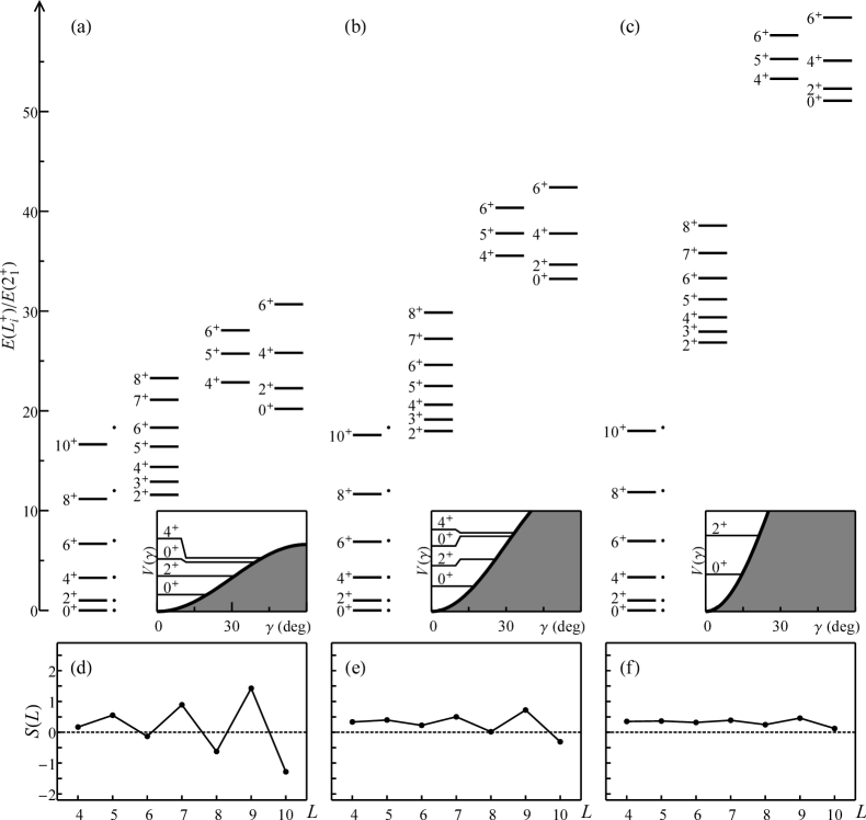
Figure 2: Level schemes for the angular Hamiltonian (5) with $\xi=0$, for (a) $\chi=50$, (b) $\chi=100$, and (c) $\chi=200$. Rotational $L(L+1)$ energies for the yrast band are indicated by the dots. The potential $V(\gamma)$ is shown in the inset, with the ground, quasi-$\gamma$, and quasi-$\gamma\gamma$ bandhead energies indicated. (d–f) Staggering of level energies within the quasi-$\gamma$ band, as measured by the energy second difference $S(L)$.

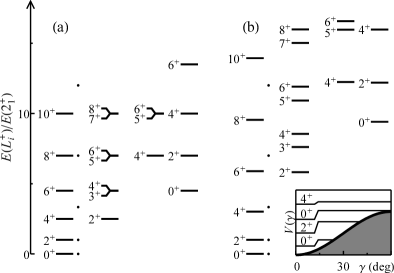
Figure 3: Level schemes for the angular Hamiltonian (5) with $\xi=0$, for (a) the $\gamma$-independent limit $\chi=0$ and (b) $\chi=20$, with levels arranged anticipating the quasiband structure of Fig. 2. Rotational $L(L+1)$ energies for the yrast band are indicated by the dots. The potential $V(\gamma)$ for $\chi=20$ is shown in the inset, with the ground, quasi-$\gamma$, and quasi-$\gamma\gamma$ bandhead energies indicated.

The nature of the spectra obtained from the Hamiltonian (5) depends both on the depth of the potential (determined by $\chi$) and the shape of the potential (determined by $\xi$ as in Fig. 1). The depth of the potential effectively controls the degree of $\gamma$ confinement. It is worth first carefully considering the implications of $\gamma$ confinement, or conversely $\gamma$ softness, within this Bohr Hamiltonian framework. In this section, we shall therefore investigate the structural dependence on $\chi$ (for $\xi=0$), before proceeding to the dependence of structure on the shape of the potential, and in particular the onset of rigid triaxiality, in Sec. IV.

The results of illustrative calculations are shown in Fig. 2, for $\chi=50$, $100$, and $200$. The low-lying states form quasi-bands which may be roughly identified as a ground-state rotational band ($K=0$), $\gamma$ vibrational excitation ($K=2$), and two-phonon $\gamma$ excitations ($K=4$ and $0$), denoted by $\gamma\gamma_{4}$ and $\gamma\gamma_{0}$.

The stiffness of the potential around $\gamma=0^{\circ}$ simultaneously determines both the $\gamma$-vibrational energy scale [increasing from Fig. 2(a) to Fig. 2(c)] and also how well confined the wave function is with respect to $\gamma$, as seen in the corresponding approach to an ideal rotational spectrum. Thus, within the framework of the Bohr Hamiltonian, the $\gamma$ band energy — more specifically, the energy ratio $E(2^{+}_{\gamma})/E(2^{+}_{1})$, or separation of vibrational and rotational energy scales — and the $\gamma$ softness of the wave function are inextricably linked.

As a starting point, it may be observed that for $\chi=0$ the potential is strictly $\gamma$-independent, and the spectrum therefore follows an $\mathrm{SO}(5)$ multiplet structure wilets1956:oscillations ; rakavy1957:gsoft . Successive multiplets consist of angular momenta $0$, $2$, $4$-$2$, $6$-$4$-$3$-$0$, $\ldots$, for $v=0$, $1$, $2$, $3$, $\ldots$, respectively, with multiplet energies $\propto v(v+3)$, as depicted in Fig. 3(a). The system is simply a Wilets-Jean wilets1956:oscillations or $\mathrm{SO}(6)$ arima1979:ibm-o6 rotor, but without $\beta$ excitations (see also Ref. rowe2004:tractable-collective ). Then, as $\gamma$ confinement is introduced, the familiar rotational band structure begins to emerge. An intermediate spectrum, obtained for $\chi=20$, is shown in Fig. 3(b).

For $\chi=50$ [Fig. 2(a)], rotational quasi-bands are well-developed, and $E(2^{+}_{\gamma})/E(2^{+}_{1})\approx 10$, as appropriate to, e.g., the well-deformed rare earth nuclei. However, it is seen from the potential plot in Fig. 2(a) that the $\gamma$ confinement for this value of $\chi$ is still weak. The range of energetically accessible $\gamma$ values increases significantly for successive phonon excitations, such that confinement is almost nonexistent at the energy of the two-phonon excitation.

Dynamical $\gamma$ deformation consequently plays a major role in the calculated structure, through its interaction with the rotational dynamics. This is reflected in significant deviations from ideal rotational behavior in the spectroscopic predictions.

Most noticeably, on inspection of Fig. 2(a), level energies within the $\gamma$ quasi-band follow a gently $\gamma$-soft staggering pattern [$2(34)(56)\ldots$]. This staggering is reminiscent of the $\mathrm{SO}(5)$ level degeneracies obtained for $\chi=0$, and it disappears as the $\gamma$ stiffness increases [Fig. 2(b,c)]. The deviations from rotational energy spacings are even more pronounced for the calculated two-phonon bands. Note especially the near doubling of the rotational energy spacing scale for the two-phonon bands, relative to the ground state band, for $\chi=50$ [Fig. 2(a)].

The deviations from rotational energy spacings within the $\gamma$ band may be seen most clearly from plots of the level energy second difference $S(L)\equiv\bigl{[}[E(L)-E(L-1)]-[E(L-1)-E(L-2)]\bigr{]}/E(2^{+}_{1})$, as shown in Fig. 2(d–f). For an ideal rotational band with $L(L+1)$ energy spacings, the curve is flat, with $S(L)=1/3$. Alternatively, $\gamma$-soft staggering is manifest in minima at even $L$. As surveyed in Ref. mccutchan2007:gamma-staggering , the observed level energies within the $\gamma$ bands of most transitional and rotational nuclei yield $S(L)$ plots which are either gently $\gamma$-soft or near constant ($\approx 1/3$). A few transitional nuclei (e.g., $\isotope[152]{Sm}$, $\isotope[156]{Gd}$, or $\isotope[162]{Er}$) exhibit a degree of staggering comparable to that found for $\chi=50$ (see also Refs. caprio2005:axialsep ; dusling2006:160er-fusevap ). However, most rare earth rotational nuclei (see Fig. 3 of Ref. mccutchan2007:gamma-staggering ) more clearly follow an $L(L+1)$ energy spacing within the $\gamma$ band. There is thus an apparent disagreement between the degree of dynamical $\gamma$ softness expected in the Bohr picture given $E(2^{+}_{\gamma})/E(2^{+}_{1})\approx 10$, and the observed structure in nuclei, at least if we assume the basic Hamiltonian (5).

Within the ground state band, the Hamiltonian (5) is found to yield relative energies [i.e., $E(L^{+}_{1})/E(2^{+}_{1})$] which fall below the $L(L+1)$ expectation for an adiabatic rotor. The ideal rotational energies are indicated, for comparison, by the dots in Fig. 2(a–c). The deviation from $L(L+1)$ spacing within the ground state band decreases, as would be expected, for increasing $\gamma$ stiffness. The effect has already been noted in the context of a full $\beta$ and $\gamma$ calculation with the ACM in Ref. rowe2009:acm (see Fig. 5 of that reference). Such a deviation would traditionally be characterized as “centrifugal stretching”, based on an the interpretation in which the $\beta$ deformation increases, and thus the rotational moments increase, with increasing angular momentum. However, here the effect is seen to arise purely from the interaction of $\gamma$ and rotational degrees of freedom, for a system in which “stretching” in the $\beta$ degree of freedom is strictly impossible.

III.2 Evolution of observables

Figure 4: Evolution of spectroscopic properties with $\gamma$ stiffness, for the angular Hamiltonian (5) with $\xi=0$. Quantities shown are (a) excitation energies of low-lying levels, normalized to $E(2^{+}_{1})$, (b) the energy ratio $E(4^{+}_{1})/E(2^{+}_{1})$, specifically, (c) electric quadrupole moments of the ground state band and $\gamma$ band $2^{+}$ members, (d) electric quadrupole reduced transition probabilities for one-phonon transitions between the ground, $\gamma$, and two-phonon $\gamma$ ($K=0$ and $4$) bandhead states, and (e) reduced transition probabilities for the transitions depopulating the $2^{+}_{\gamma}$ bandhead state. All electromagnetic quantities are normalized to $B(E2;2^{+}_{1}\rightarrow 0^{+}_{1})\equiv 1$.

The evolution of the numerical predictions, with increasing $\gamma$ stiffness, is examined more quantitatively and systematically in Fig. 4. Both the energy spectrum [Fig. 4(left)] and electromagnetic (specifically, electric quadrupole) moments and transition matrix elements [Fig. 4(right)] are shown, as functions of $\chi$.

The onset and evolution of rotational band structure, as $\gamma$ confinement is introduced, may be traced in the full energy spectrum [Fig. 4(a)]. Note especially the correlation between the $\gamma$ band energy [Fig. 4(a)] and the ground state band energy ratio $E(4^{+}_{1})/E(2^{+}_{1})$ [Fig. 4(b)], which varies from $2.5$ for $\gamma$-independent rotation to $3.33$ for rigid axial rotation. This ratio is commonly taken as an indicator of rotational adiabaticity. For the present restricted problem, adiabaticity represents separation of the $\gamma$ and rotational degrees of freedom, but in general for the Bohr Hamiltonian the quantitative details will also be affected by the $\beta$ degree of freedom. The evolution of multiphonon band energies can also be followed in Fig. 4. These begin anharmonically low, at less than twice the $\gamma$ band energy — for $\chi=50$, an estimate based on low-lying band members gives $E_{\gamma\gamma,4}/E_{\gamma}\approx 1.7$ and $E_{\gamma\gamma,0}/E_{\gamma}\approx 1.9$ — but approach harmonicity as $\chi$ increases. The relative energies of the bands may also be seen in Fig. 2(a–c).

The evolution of electromagnetic properties is traced for representative quadrupole moments and transition strengths in Fig. 4(right). In the $\gamma$-independent limit, the wave functions are simply the $\mathrm{SO}(5)\supset\mathrm{SO}(3)$ spherical harmonics themselves, and electromagnetic matrix elements are governed by $\mathrm{SO}(5)$ selection rules and related by $\mathrm{SO}(5)\supset\mathrm{SO}(3)$ Clebsch-Gordan coefficients. On the other hand, in the limit of large $\gamma$ stiffness, electromagnetic matrix elements are expected to approach the Alaga rule ratios alaga1955:branching ; bohr1998:v2 of the adiabatic axial rotor, given by ordinary angular momentum Clebsch-Gordan coefficients.

The electric quadrupole moments $Q(2^{+}_{1})$ and $Q(2^{+}_{\gamma})$ are shown in Fig. 4(c). All quadrupole moments vanish in the $\gamma$-independent limit, by a selection rule arising from a parity quantum number defined in the five-dimensional space of the Bohr coordinates ($\mathbb{R}^{5}$-parity) bes1959:gamma ; rowe2009:acm ; caprio2009:gammaharmonic . In the rotational limit, these quadrupole moments are expected to approach values of $\pm 8\sqrt{\pi}/7\approx\pm 2.03$, negative for the ground state band ($K=0$) and positive for the $\gamma$ band ($K=2$), expressed relative to $B(E2;2^{+}_{1}\rightarrow 0^{+}_{1})^{1/2}$. These values are rapidly attained, by $\chi\lesssim 25$.

For harmonic $\gamma$ vibration, the $\gamma\rightarrow g$, $\gamma\gamma_{4}\rightarrow\gamma$, and $\gamma\gamma_{0}\rightarrow\gamma$ interband intrinsic matrix elements $\langle{f}|{\mathcal{M}^{\prime}}|{i}\rangle$ bohr1998:v2 are expected to be in the proportion $1:\sqrt{2}:1$ rowe2010:rowanwood . The overall normalization of these intrinsic matrix elements, i.e., the $\gamma\rightarrow{}g$ strength, decreases with increasing $\gamma$ stiffness eisenberg1987:v1 . For the transitions among the bandhead states, in particular, these intrinsic matrix element ratios correspond to $B(E2;2^{+}_{\gamma}\rightarrow 0^{+}_{g})$, $B(E2;4^{+}_{\gamma\gamma,4}\rightarrow 2^{+}_{\gamma})$, and $B(E2;0^{+}_{\gamma\gamma,0}\rightarrow 2^{+}_{\gamma})$ strengths in the proportion $1:2.8:5$. The approach to harmonic values is seen in Fig. 4(d). Simply from considering these transitions, harmonic behavior would appear to set in very gradually for $\chi\gtrsim 50$. However, a more comprehensive consideration of the electromagnetic transition strengths, which leads to some modification of this conclusion, is provided by the Mikhailov analysis in Sec. III.4. The branching ratios for electric quadrupole transitions between bands likewise approach the Alaga rule ratios. For the transitions from the $2^{+}_{\gamma}$ bandhead to the ground state band members [Fig. 4(e)], for instance, the adiabatic rotor has $B(E2;2^{+}_{\gamma}\rightarrow 0^{+}_{g})$, $B(E2;2^{+}_{\gamma}\rightarrow 2^{+}_{g})$ and $B(E2;2^{+}_{\gamma}\rightarrow 4^{+}_{g})$ strengths in the proportion $0.4:0.57:0.029$.

III.3 Effective $\gamma$ deformation

Figure 5: Evolution of the effective values $\bar{\gamma}$ with respect to stiffness parameter $\chi$, for the angular Hamiltonian (5) with $\xi=0$. Values are shown for ground state, $\gamma$, $\gamma\gamma_{4}$, and $\gamma\gamma_{0}$ quasi-band members with $L\leq 4$.

Although we have so far examined $\gamma$ softness indirectly, through its spectroscopic signatures, the wave function $\psi(\gamma,\Omega)$ is directly accessible for the eigenstates calculated in the diagonalization of the Bohr Hamiltonian, and thus the deviation of $\gamma$ from $0^{\circ}$ can be considered directly. The simplest measure is provided by an effective $\gamma$ value $\bar{\gamma}$, defined by

$$\cos 3\bar{\gamma}\equiv\langle\cos 3\gamma\rangle.$$ (10)

The matrix elements of $\cos 3\gamma$ in the $\mathrm{SO}(5)\supset\mathrm{SO}(3)$ spherical harmonic basis are already available, as noted in Sec. II, so this expectation value may readily be calculated. The definition (10) is consistent with the quadrupole shape invariant approach kumar1972:q-invariant ; cline1986:coulex , in which an effective $\gamma$ for the full $(\beta,\gamma,\Omega)$ coordinate space is defined by $\cos 3\gamma_{\text{eff}}=\langle\beta^{3}\cos 3\gamma\rangle/\langle\beta^{2}\rangle^{3/2}$ elliott1986:ibm-shape ; jolos1997:ibm-shape-invariant ; werner2005:triax-invariant .

The evolution of $\bar{\gamma}$ for the ground state, $\gamma$, and $\gamma\gamma$ band members (for $L\leq 4$) is shown in Fig. 5. In the $\chi=0$ ($\gamma$-independent) limit, $\langle\cos 3\gamma\rangle=0$ by the $\mathbb{R}^{5}$-parity selection rule, and thus $\bar{\gamma}=30^{\circ}$ for all states. As $\chi$ increases past $\chi\approx 50$, it is seen that the $\bar{\gamma}$ values for the members of each band cluster and decrease with increasing $\chi$. The $\bar{\gamma}$ value jumps substantially between bands, increasing from ground to $\gamma$ to $\gamma\gamma$ bands, indeed, as expected for successive phonon excitations.

The situation for “axial rotor” nuclei within the Bohr Hamiltonian framework is very much contrary to the classic but schematic characterization of such nuclei as having “$\gamma\approx 0^{\circ}$”, which may be more concretely interpreted as $\gamma\ll 30^{\circ}$. Recall that the $\gamma$-band excitation energies matching the experimental values for rotor nuclei are obtained for $\chi\approx 50$. For this stiffness, the ground state band members have $\bar{\gamma}\approx 15^{\circ}$, and the $\gamma$ band members have $\bar{\gamma}\approx 23^{\circ}$. These large $\bar{\gamma}$ values are consistent with the large range of energetically accessible $\gamma$ values for these states [Fig. 2(a,inset)]. The full probability distribution with respect to the $\gamma$ coordinate is considered in Sec. V.

III.4 Intrinsic matrix elements

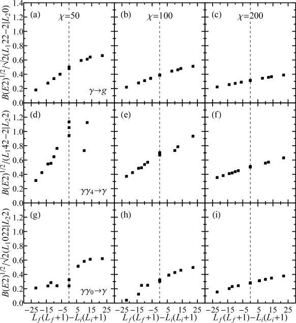
Figure 6: Interband transition amplitudes $B(E2)^{1/2}$, from the $\gamma$ quasi-band to the ground state band (top), from the $\gamma\gamma_{4}$ quasi-band to the $\gamma$ quasi-band (middle), and from the $\gamma\gamma_{0}$ quasi-band to the $\gamma$ quasi-band (bottom), for Mikhailov analysis. Plots are included for the calculations of Fig. 2, with $\chi=50$ (left), $\chi=100$ (middle), and $\chi=200$ (right) and $\xi=0$. The values shown are for transitions between levels with $L\leq 6$, normalized to $B(E2;2^{+}_{1}\rightarrow 0^{+}_{1})\equiv 1$.

Table 1: Electric quadrupole interband intrinsic matrix elements $\langle{f}|{\mathcal{M}^{\prime}}|{i}\rangle$ and mixing parameters $a$, for different $\gamma$ stiffnesses, as extracted from the Mikhailov analyses of Fig. 6. Ratios, as indicators of anharmonicity, are tabulated in the final two columns. The values for an adiabatic rotor with harmonic $\gamma$ vibration rowe2010:rowanwood are included for comparison. The values for the intrinsic matrix elements are normalized to $B(E2;2^{+}_{1}\rightarrow 0^{+}_{1})\equiv 1$.

	$\gamma\rightarrow g$		$\gamma\gamma_{4}\rightarrow\gamma$		$\gamma\gamma_{0}\rightarrow\gamma$
	$\langle{f}|{\mathcal{M}^{\prime}}|{i}\rangle$	$a$	$\langle{f}|{\mathcal{M}^{\prime}}|{i}\rangle$	$a$	$\langle{f}|{\mathcal{M}^{\prime}}|{i}\rangle$	$a$	$\dfrac{\gamma\gamma_{4}\rightarrow\gamma}{\gamma\rightarrow g}$	$\dfrac{\gamma\gamma_{0}\rightarrow\gamma}{\gamma\rightarrow g}$
$\chi=50$a	$0.42$	$0.025$	$\sim 0.6^{a}$	$\sim 0.03$	$\sim 0.5^{a}$	$\sim 0.03$	$\sim 1.4^{a}$	$\sim 1.1^{a}$
$\chi=100$	$0.30$	$0.012$	$0.43$	$0.012$	$0.30$	$0.018$	$1.44$	$1.01$
$\chi=200$	$0.23$	$0.007$	$0.33$	$0.007$	$0.23$	$0.009$	$1.43$	$1.00$
Harmonic	—		—		—		$1.41$	$1$

^a The $\gamma\gamma\rightarrow\gamma$ intrinsic matrix elements for $\chi=50$ can only be crudely approximated, since the Mikhailov plot yields values which are not strongly linear [Fig. 6(d,g)]. The estimated parameters used in the analysis are $M_{1}\approx 0.9$ for $\gamma\gamma_{4}\rightarrow\gamma$ and $M_{1}\approx 0.4$ for $\gamma\gamma_{0}\rightarrow\gamma$.

A more comprehensive and meaningful examination of electromagnetic transition strengths is realized by considering the interband transitions in aggregate, according to the Mikhailov mixing formalism mikhailov1966:mixing-APS . Within this framework, all transition amplitudes are expressed in terms of a single intrinsic electromagnetic matrix element and single mixing parameter between each pair of bands. The amplitudes are expected to fall on a straight line on an appropriate (Mikhailov) plot of $\langle K_{2}J_{2}\|\mathcal{M}\|K_{1}J_{1}\rangle$ or, commonly, $B(E2)^{1/2}$ vs. $J_{2}(J_{2}+1)-J_{1}(J_{1}+1)$. The intrinsic matrix elements and mixing parameter are identified from the slope and intercept.

Specifically, for interband transitions with $\Delta K=2$, the leading-order band mixing relation for $E2$ reduced matrix elements is (bohr1998:v2, , (4-210))

$$\langle K_{2}J_{2}\|\mathcal{M}\|K_{1}J_{1}\rangle=\sigma_{1}(2J_{1}+1)^{1/2}(J_{1}K_{1}22|J_{2}K_{2})\\ \times\bigl{[}M_{1}+M_{2}[J_{2}(J_{2}+1)-J_{1}(J_{1}+1)]\bigr{]},$$ (11)

where it is assumed that $K_{2}=K_{1}+2$, and where $\sigma_{1}=\sqrt{2}$ if $K_{1}=0$ or $\sigma_{1}=1$ otherwise. The parameters in this expression are related to the intrinsic matrix element $\langle{K_{2}}|{\mathcal{M}^{\prime}}|{K_{1}}\rangle$, mixing matrix element $\langle{K_{2}}|{\varepsilon_{+2}}|{K_{1}}\rangle$, and intrinsic quadrupole moment $Q_{0}$ by $M_{1}=\langle{K_{2}}|{\mathcal{M}^{\prime}}|{K_{1}}\rangle-4(K_{1}+1)M_{2}$ and $M_{2}=[15/(8\pi)]^{1/2}eQ_{0}\langle{K_{2}}|{\varepsilon_{+2}}|{K_{1}}\rangle$ (bohr1998:v2, , (4-211)). The intrinsic matrix element may thus be extracted from the slope and intercept as

$$\langle{K_{2}}|{\mathcal{M}^{\prime}}|{K_{1}}\rangle=M_{1}+4(K_{1}+1)M_{2}.$$ (12)

More specific expressions for $K$-decreasing and $K$-increasing transitions, in terms of $B(E2)$ reduced transition probabilities, are given in Appendix B.

The interband quadrupole transition strengths for the Bohr Hamiltonian calculations of Sec. III.1 are shown in Fig. 6 in Mikhailov form. They are plotted as $B(E2)^{1/2}$ vs. $L_{f}(L_{f}+1)-L_{i}(L_{i}+1)$, for transitions between states with $L\leq 6$. For the most part, the transition amplitudes do indeed follow an essentially linear pattern, and it is therefore meaningful to extract effective intrinsic matrix elements, well as mixing parameters, from the Mikhailov analysis. (The Mikhailov formalism has been applied to extract effective intrinsic matrix elements from the interacting boson model iachello1987:ibm , in a similar fashion, in Refs. warner1981:168er-ibm ; aprahamian2006:162dy-grid .) However, deviations from a linear relation are significant for transitions involving the two-phonon quasi-bands for $\chi=50$ [Fig. 6(left)], as might be expected from the substantial $\gamma$-softness and deviations from rotational energy spacings already noted for these bands. The resulting intrinsic matrix elements for the $\gamma\rightarrow g$, $\gamma\gamma_{4}\rightarrow\gamma$, and $\gamma\gamma_{0}\rightarrow\gamma$ transitions, obtained from (17) and (19), are listed in Table 1, together with the dimensionless mixing parameter $a=\lvert M_{2}/M_{1}\rvert$ (see Appendix B). The normalization of the electric quadrupole operator $\mathcal{M}(E2)$ is arbitrary in the present analysis. To provide a scale for comparison with experiment, the intrinsic matrix elements in Table 1 are given relative to the square root of the in-band $B(E2;2^{+}_{1}\rightarrow 0^{+}_{1})$.

For harmonic $\gamma$ vibration, the ratios of the $\gamma\gamma\rightarrow\gamma$ intrinsic matrix elements to the $\gamma\rightarrow g$ intrinsic matrix element are expected to be $\langle{\gamma}|{\mathcal{M}^{\prime}}|{\gamma\gamma_{4}}\rangle/\langle{g}|{\mathcal{M}^{\prime}}|{\gamma}\rangle=\sqrt{2}\approx 1.41$ and $\langle{\gamma}|{\mathcal{M}^{\prime}}|{\gamma\gamma_{0}}\rangle/\langle{g}|{\mathcal{M}^{\prime}}|{\gamma}\rangle=1$, according to the proportion noted in Sec. III.2. For comparison, ratios of the intrinsic matrix elements extracted from the Bohr Hamiltonian numerical calculations are given in the last two columns of Table 1. Note the rapid quantitative approach of these calculated ratios to the expected harmonic values. Even the $\gamma\gamma\rightarrow\gamma$ transitions for the soft $\chi=50$ case are essentially consistent with harmonic ratios, to the extent that slope and intercept parameters can meaningfully be extracted in this instance [Fig. 6(d,g)]. For $\chi=200$, harmonic values are obtained to within $\sim 1\%$.

The bandmixing, indicated by the Mikhailov plot slopes, is substantial in all the cases considered in Table 1. The harmonicity of the intrinsic matrix elements is therefore not apparent simply from the plot intercepts buy only after the leading-order bandmixing corrections (17) and (19) are taken into account. For example, even for the most adiabatic case, $\chi=200$, the $\gamma\rightarrow g$ [Fig. 6(c)]and $\gamma\gamma_{4}\rightarrow\gamma$ [Fig. 6(f)] Mikhailov plots both have slope parameters $a\approx 0.012$, resulting in a $5\%$ adjustment to the $\gamma\rightarrow g$ intrinsic matrix element and a $14\%$ adjustment to the $\gamma\gamma_{4}\rightarrow\gamma$ intrinsic matrix element.

In summary, although the strengths of the individual interband transitions only approach the limit of an adiabatic rotor (and, more specificially, harmonic vibration) gradually, as observed from Fig. 4(d), this deviation is quantitatively well-described in terms of a rapid approach to harmonic values of the interband intrinsic matrix elements, but with the individual transition strengths modified by leading-order $\Delta K=2$ bandmixing (11). The strength of this mixing then gradually decreases with increasing $\gamma$ stiffness.

IV Onset of rigid triaxiality

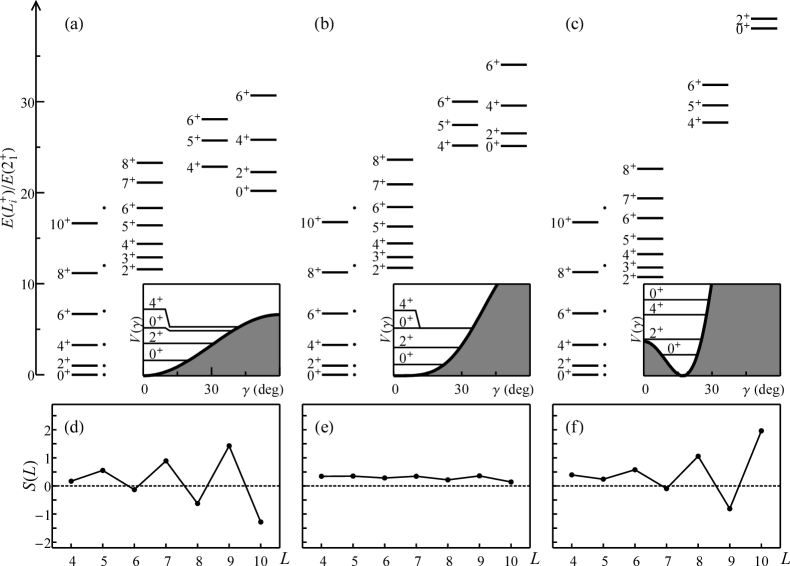
Figure 7: Level schemes for the angular Hamiltonian (5), for (a) $\xi=0$ with $\chi=50$, (d) $\xi=0.5$ with $\chi=100$, and (e) $\xi=0.8$ with $\chi=500$. Rotational $L(L+1)$ energies for the yrast band are indicated by the dots. The potential $V(\gamma)$ is shown in the inset, with the ground, quasi-$\gamma$, and quasi-$\gamma\gamma$ bandhead energies indicated. (d–f) Staggering of level energies within the quasi-$\gamma$ band, as measured by the energy second difference $S(L)$. Figure adapted from Ref. caprio2009:gammaharmonic .

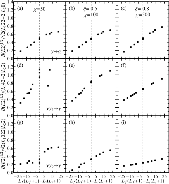
Figure 8: Interband transition amplitudes $B(E2)^{1/2}$, from the $\gamma$ quasi-band to the ground state band (top), from the $\gamma\gamma_{4}$ quasi-band to the $\gamma$ quasi-band (middle), and from the $\gamma\gamma_{0}$ quasi-band to the $\gamma$ quasi-band (bottom), for Mikhailov analysis. Plots are included for the calculations of Fig. 7, with $\xi=0$ ($\chi=50$) (left), $\xi=0.5$ ($\chi=100$) (middle), and $\xi=0.8$ ($\chi=500$) (right). The values shown are for transitions between levels with $L\leq 6$, normalized to $B(E2;2^{+}_{1}\rightarrow 0^{+}_{1})\equiv 1$. Figure panels (a–f) adapted from Ref. caprio2009:gammaharmonic .

Table 2: Electric quadrupole interband intrinsic matrix elements $\langle{f}|{\mathcal{M}^{\prime}}|{i}\rangle$ and mixing parameters, for different $\gamma$ potential shapes chosen to reproduce the onset of weak rigid triaxiality, as extracted from the Mikhailov analyses of Fig. 8. Ratios, as indicators of anharmonicity, are tabulated in the final two columns. The $\mathrm{Y}(5)$ triaxial estimate iachello2003:y5 is included for comparison. The values for the intrinsic matrix elements are normalized to $B(E2;2^{+}_{1}\rightarrow 0^{+}_{1})\equiv 1$. The results in this table also serve to correct intrinsic matrix element values given previously in Table 1 of Ref. caprio2009:gammatriax . The roles of initial and final bands were interchanged, in that analysis, when extracting the slope parameter from (16) and (18), resulting in the use of an incorrect sign for the bandmixing correction term in (17) and (19).

	$\gamma\rightarrow g$		$\gamma\gamma_{4}\rightarrow\gamma$		$\gamma\gamma_{0}\rightarrow\gamma$
	$\langle{f}|{\mathcal{M}^{\prime}}|{i}\rangle$	$a$	$\langle{f}|{\mathcal{M}^{\prime}}|{i}\rangle$	$a$	$\langle{f}|{\mathcal{M}^{\prime}}|{i}\rangle$	$a$	$\dfrac{\gamma\gamma_{4}\rightarrow\gamma}{\gamma\rightarrow g}$	$\dfrac{\gamma\gamma_{0}\rightarrow\gamma}{\gamma\rightarrow g}$
$\xi=0.5$ ($\chi=100$)	$0.43$	$0.025$	$0.58$	$0.022$	$0.37$	$0.035$	$1.36$	$0.87$
$\xi=0.8$ ($\chi=500$)	$0.43$	$0.028$	$0.51$	$0.018$	$0.27$	$0.015$	$1.18$	$0.63$
$\mathrm{Y}(5)$	—		—		—		$1.23$	$0.73$

The excitation spectrum may be expected to change dramatically with the onset of rigid triaxiality. The Bohr Hamiltonian predictions ultimately approach a $\gamma=30^{\circ}$ Davydov rotor spectrum davydov1958:arm-intro for confinement by a sufficiently stiff $\cos^{2}3\gamma$ potential rowe2009:acm . However, the initial onset of triaxiality is reflected in much more subtle deviations from the characteristics of an axially symmetric rotor. The difference between axial and triaxial minima in the potential is obscured by the substantial dynamical fluctuations in $\gamma$ present in both cases. As noted in Sec. II, the onset of triaxiality may be investigated by considering the introduction of a $\cos^{2}3\gamma$ contribution, i.e., nonzero $\xi$, in the Hamiltonian (5).

The results of calculations for two representative potentials are shown in Fig. 7: the soft or “critical” axial minimum ($\xi=0.5$) [Fig. 7(b)] and a weakly triaxial minimum ($\xi=0.8$) [Fig. 7(c)]. For each of these calculations, the potential depth, or $\chi$, is chosen to give $E(2^{+}_{\gamma})/E(2^{+}_{1})\approx 10$, again appropriate to the well-deformed rare earth nuclei. The comparable axial rotor calculation with the same $\gamma$ band energy, i.e., $\chi=50$, is shown again as a baseline for comparison [Fig. 7(a)].

In Fig. 7, the $\gamma$-phonon quasiband structure is seen to remain intact. Our concern is therefore with the principal spectroscopic properties of these bands — excitation energies of the bands, deviations from rotational energy spacing within the bands, and electric quadrupole intrinsic matrix elements. The two-phonon energy anharmonicities evolve from slightly negative ($E_{\gamma\gamma}/E_{\gamma}<2$) for $\xi=0$ [Fig. 7(a)] to positive ($E_{\gamma\gamma}/E_{\gamma}>2$) [Fig. 7(b,c)] with the introduction of triaxial tendencies. The anharmonicity of the $\gamma\gamma_{0}$ band rises more rapidly than that of the $\gamma\gamma_{4}$ quasi-band. Qualitatively, this is consistent with evolution towards a $\gamma$-stiff, adiabatic triaxial rotor rowe2010:rowanwood , for which the $K=4$ quasi-band is a triaxial rotational excitation and the $K=0$ quasi-band is a $\gamma$ vibrational excitation.

The level energies within the $\gamma$ band progress, with increasing $\xi$, from $\gamma$-soft staggering [$2(34)(56)\ldots$] to the reverse pattern associated with triaxial rotation [$(23)(45)\ldots$] davydov1958:arm-intro . As in Sec. III.1, the staggering may be seen most immediately from plots of the second difference $S(L)$ [Fig. 7(d–f)], which has minima at even $L$ for $\gamma$-soft staggering or at odd $L$ for triaxial staggering.

The “centrifugal stretching” phenomenon in the yrast band, i.e., reduction of $E(L^{+}_{1})/E(2^{+}_{1})$ relative to $L(L+1)$ spacing, persists [Fig. 7(b,c)] at about the same level as for $\chi=50$. However, the growth in rotational constant (and general deviation from rotational behavior) for the excited, especially $\gamma\gamma$, bands is tamed relative to the axial calculation. This may be at least qualitatively understood by comparing the potential plots in Fig. 7(a–c,insets). The axial calculation of Fig. 7(a), as noted in Sec. III.1, provides only weak confinement at the $\gamma\gamma$ band energies ($\gamma\lesssim 40^{\circ}$). Although the nominally “softer” calculation of Fig. 7(b) does provide weaker confinement, compared to this axial calculation, at the ground state energy, it actually provides stiffer confinement, to a smaller range of $\gamma$ values ($\gamma\lesssim 30^{\circ}$), at the $\gamma\gamma$ band energies. [This effect may be more properly considered a reflection of the steep rise in the $\cos^{2}3\gamma$ term used to create the triaxial confinement than an intrinsic property of the onset of triaxiality per se. There is no inherent calculational reason not to consider a potential with, for instance, a triaxial minimum located at the same position as in Fig. 7(c,inset) but a lower barrier at $\gamma=60^{\circ}$.] A similar observation may be made for the calculation of Fig. 7(c), which provides confinement to triaxial $\gamma$ at the ground state energy, but simply provides (axial) confinement to $\gamma\lesssim 30^{\circ}$ at the $\gamma\gamma$ band energies.

For the weakly triaxial calculations considered here, the interband transition strengths continue to follow an essentially linear pattern on a Mikhailov plot, as expected for rotational bandmixing, as seen in Fig. 8. The $\gamma\gamma\rightarrow\gamma$ transitions, in fact, demonstrate better linear behavior [Fig. 8(e–f,h–i)] than for $\chi=50$ [Fig. 8(d,g)]. Interband intrinsic matrix elements may therefore again be extracted from the Mikhailov analysis, as given in Table 2. The $\gamma\rightarrow g$ intrinsic matrix element remains essentially constant, and equal to that for the axial $\chi=50$ calculation, but the $\gamma\gamma_{4}\rightarrow\gamma$, and $\gamma\gamma_{0}\rightarrow\gamma$ intrinsic matrix elements decrease substantially compared to the harmonic $\gamma$-vibrational values.

Such a reduction of the $\gamma\gamma\rightarrow\gamma$ intrinsic matrix elements, relative to the harmonic values, has already been proposed iachello2003:y5 on relatively simple grounds. Supposing an adiabatic separation of rotation from vibration, and furthermore imposing a small-$\gamma$ approximation, yields a one-dimensional Schrödinger equation problem in $\gamma$. In Ref. iachello2003:y5 , a square well is then adopted for $V(\gamma)$ to simulate the onset of triaxiality. This yields the $\mathrm{Y}(5)$ estimate shown for comparison in Table 2.

V Wave function probability distributions

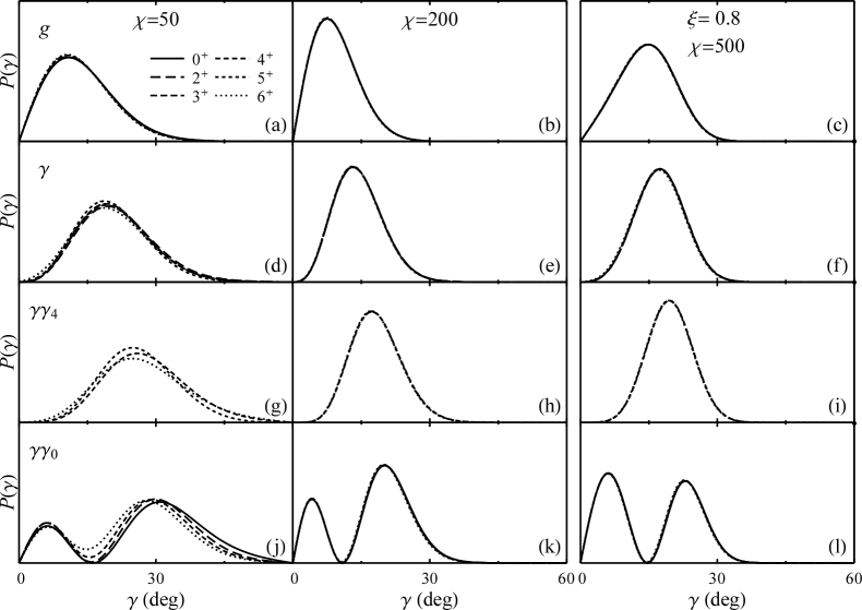
Figure 9: Probability distributions with respect to $\gamma$ for low-lying quasi-band members in calculations with Hamiltonian (5), for the axial cases $\chi=50$ (left) and $\chi=200$ (middle), both with $\xi=0$, and for the weakly triaxial case $\xi=0.8$ with $\chi=500$ (right). Probability distributions are shown for members of the ground state, $\gamma$, $\gamma\gamma_{4}$, and $\gamma\gamma_{0}$ quasi-bands (top to bottom, respectively), with $L\leq 6$.

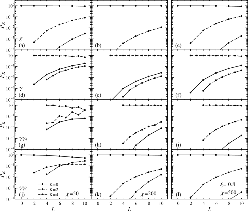
Figure 10: The $K$ content of low-lying quasi-band members in calculations with Hamiltonian (5), for the axial cases $\chi=50$ (left) and $\chi=200$ (middle), both with $\xi=0$, and for the weakly triaxial case $\xi=0.8$ with $\chi=500$ (right). Probabilities $P_{K}$ for $K=0$ (solid curve), $K=2$ (dashed curve), and $K=4$ (dotted curve) are shown for members of the ground state, $\gamma$, $\gamma\gamma_{4}$, and $\gamma\gamma_{0}$ quasi-bands (top to bottom, respectively), with $L\leq 10$.

In the limit of adiabatic separation of the $\gamma$ and rotational degrees of freedom, the wave functions of all members of a band would be given by

$$\psi_{KLM}(\gamma,\Omega)=F_{K}(\gamma)\xi^{(L)}_{KM}(\Omega),$$ (13)

where the function $F_{K}(\gamma)$ would be identical for all states within the same band, independent of $L$. The band is characterized by intrinsic angular momentum projection $K$. This may be contrasted to the general situation (6), in which all even $K$ with $0\leq K\leq L$ (or $2\leq K\leq L$ for $L$ odd) can contribute, and the coefficients $F_{K}(\gamma)$ need not be directly related for different states. The breaking of adiabaticity has already been seen to have spectroscopic consequences (Secs. III and IV). Here we shall more directly inspect the wave functions themselves, through the probability distributions. Specifically, we examine the probability distribution $P(\gamma)$, with respect the $\gamma$ coordinate, after integration over Euler angles, and the probability decomposition $P_{K}$, with respect to the $K$ quantum number for the Euler angle (rotational) dependence, after integration over $\gamma$. The calculational details are given in Appendix C.

First, considering $P(\gamma)$, results are given in Fig. 9 for the softest axial calculation of Sec. III ($\chi=50$) [Fig. 9(left)], the stiffest axial calculation of Sec. III ($\chi=200$) [Fig. 9(middle)], and the weakly triaxial calculation of Sec. IV ($\xi=0.8$ with $\chi=500$) [Fig. 9(right)]. Successive panels (top to bottom) show the $P(\gamma)$ distributions for the ground, $\gamma$, $\gamma\gamma_{4}$, and $\gamma\gamma_{0}$ band members, respectively, with $L\leq 6$. All the $P(\gamma)$ vanish at $\gamma=0^{\circ}$ and $\gamma=60^{\circ}$, due to the volume element for the Bohr coordinates (see Appendix C).

The basic features seen in Fig. 9 may be qualitatively understood in terms of the small-$\gamma$ limit of (5), which reduces (e.g., Ref. iachello2003:y5 ) to a two-dimensional harmonic oscillator problem, with two-dimensional angular momentum $m=K/2$ and with $\gamma$ as the “radial” variable. The $K=2n_{\gamma}$ (or $m=n_{\gamma}$) bands, i.e., the ground, $\gamma$, and $\gamma\gamma_{4}$ bands, have probability distributions which are nodeless. These move towards higher $\gamma$ with increasing phonon number $n_{\gamma}$ [Fig. 9(a,d,g) or Fig. 9(b,e,h)]. The centers of the probability distributions are at substantially nonzero $\gamma$ values, in the $10^{\circ}$–$30^{\circ}$ range, but move towards smaller $\gamma$ for larger stiffess [compare Fig. 9(left) with Fig. 9(middle)]. All these properties are as anticipated from the $\bar{\gamma}$ values in Fig. 5. For the $\gamma\gamma_{0}$ band, which is characterized by $K=2(n_{\gamma}-2)$ (or $m=n_{\gamma}-2$), the probability distributions have a single node [Fig. 9(j,k)].

Adiabatic separation (13) implies identical $P(\gamma)$ distributions for all members of the same band. Indeed, the $P(\gamma)$ curves are virtually indistinguishable between band members for the examples in Fig. 9. The exceptions are, once again, the $\gamma\gamma$ bands in the $\chi=50$ calculation [Fig. 9(g,j)]. There is some slight displacement between the curves for the different members of the ground or $\gamma$ bands in this calculation as well. The breaking of adiabaticity is also apparent for the $\gamma\gamma_{0}$ band members with $L>0$, from the disappearance of the node in $P(\gamma)$, which indicates that multiple $K$ values must contribute to the wave function.

It is interesting to note the qualitative differences of the more triaxial calculation [Fig. 9(right)] from the axial calculations [Fig. 9(left,middle)]. The $P(\gamma)$ for the ground, $\gamma$, and $\gamma\gamma_{4}$ bands (i.e., those with nodeless distributions) [Fig. 9(c,f,i)] are peaked at $\gamma$ values roughly comparable to those for the $\chi=50$ “axial” calculation [Fig. 9(a,d,g)] (recall that the parameters were chosen so that these calculations share the same $\gamma$ band energy) but are more sharply peaked. The $\gamma\gamma_{0}$ distribution [Fig. 9(l)] shows a marked enhacement of the peak at small (axial) $\gamma$. This may seem counterintuitive for a “triaxial” calculation, but, as already remarked in Sec. IV, the triaxial confinement is limited to the ground state band energy.

In interpreting the $P(\gamma)$ distributions as indicators of adiabaticity, it should be noted that, although adiabatic separation implies identical $P(\gamma)$ distributions, the converse is not strictly true. Adiabaticity might be violated, and several $K$ values might contribute in (6), but the various $F_{K}(\gamma)$ for the different band members may be related such that, nonetheless, the same $P(\gamma)$ distributions are obtained after integration over Euler angles. Therefore, these distributions can only be conclusively taken to indicate adiabaticity if it is also known that only one $K$ value contributes significantly.

The contributions of different $K$ values in each of the bands (ground, $\gamma$, $\gamma\gamma_{4}$, and $\gamma\gamma_{0}$) are shown in Fig. 10, for each band member with $L\leq 10$. For the calculations in Fig. 10, the bandhead states have essentially pure $K$. The largest admixture in a bandhead state is $\sim 3\%$ for the $\gamma\gamma_{4}$ bandhead in the $\chi=50$ calculation, but the bandhead $K$ admixtures in the other calculations are all $<10^{-3}$. (Note that the $\gamma\gamma_{0}$ bandhead, as an $L=0$ state, trivially has pure $K=0$.) The admixtures increase with $L$ within each band. Again, the extremes are in the $\gamma\gamma$ bands for $\chi=50$, where the admixtures account for approximately half the probability at $L=10$ [Fig. 10(g,j)]. In contrast, for the weakly triaxial calculation [Fig. 10(right)], the $K$ admixtures in the $\gamma\gamma$ bands are actually slightly smaller than for the ground state band. Indeed, they closely match the $K$ admixtures of the corresponding bands in the stiff axial $\chi=200$ calculation [Fig. 10(middle)]. This observation is consistent with the characterization of these bands as relatively “good” axial rotational bands, as suggested spectroscopically in Sec. IV.

VI Conclusion

The possibility of exact diagonalization of the Bohr Hamiltonian for essentially arbitrary $\beta$ and $\gamma$ stiffness opens the door for direct comparison of the Bohr Hamiltonian predictions with experiment throughout the range of possible dynamics for the nuclear quadrupole degree of freedom. At a phenomenological level, this permits meaningful tests of the Bohr Hamiltonian for general rotor-vibrator nuclei.

For instance, in the past, interpretation of rotational “phonon” states, although nominally within the Bohr description, has largely been at a schematic level (e.g., Refs. gunther1967:166er-168er-beta ; riedinger1969:152sm154gd-beta ; warner1981:168er-ibm ; wu1996:gamma-fragmentation-os ; haertlein1998:168er-coulex ): adiabatic separation of the rotational and vibrational degrees of freedom is assumed, the $\beta$ and $\gamma$ excitations are taken to be harmonic, and phonon selection rules are assumed for electric quadrupole transitions. These predictions are then adjusted by the leading-order spin-dependent bandmixing relation, but with ad hoc mixing parameters. Here, instead, we explore exact predictions of the Bohr Hamiltonian, both for axial and weakly triaxial confinement.

The present analysis, which has been restricted to the $\gamma$ and rotational degrees of freedom, provides a starting point for understanding the full dynamics involving all five Bohr coordinate degrees of freedom, i.e., considering coupling with the $\beta$ degree of freedom as well. Many of the qualitative properties of the present solution may be expected to carry over (see, e.g., Fig. 4 of Ref. caprio2009:gammatriax ). However, the introduction of $\beta$ softness may generally be expected to quantitatively alter the results, for instance, further attenuating the rotational character of the bands [e.g., reducing the ratio $E(4^{+}_{1})/E(2^{+}_{1})$]. Moreover, in the case of near degeneracy of the $\gamma$ phonon or multiphonon bands with bands involving $\beta$ excitations, bandmixing can substantially alter the results. Therefore, detailed comparison with experiment should be made in the context of a full treatment incorporating $\beta$ softness.

Microscopic descriptions of nuclear collectivity rely upon a reduction of the many-body problem to one involving effective collective degrees of freedom. Mean-field approaches to deriving the quadrupole collective dynamics (reviewed in, e.g., Refs. klein1991:collective ; prochniak2009:bohr-collective-hf-hg ; matsuyanagi2010:micro-collective-problems ) yield a Hamiltonian involving a much more general, coordinate-dependent form for the kinetic energy operator than the conventional but schematic Laplacian form considered in (1). The resulting generalized Bohr Hamiltonian prochniak2009:bohr-collective-hf-hg may be represented in terms of coordinate-dependent moments of inertia. It should be noted that the ACM can readily accommodate Hamiltonians involving much more general differential operators rowe2005:radial-me-su11 in the $\beta$ and angular variables than the simple Laplacian form. For instance, scalar-coupled products of the quadrupole momentum tensor $p$ and coordinate tensor $q$ constitute an important special case considered in the geometric collective model hess1980:gcm-details-238u ; eisenberg1987:v1 . The Bohr kinetic energy is obtained as the lowest-order term $(p\times p)^{(0)}$, and attention in phenomenological studies has largely been limited to the next term $(p\times q\times p)^{(0)}$. These and higher-order terms in the coordinate dependence may be combined to recover much or all of the flexibility of the generalized Bohr Hamiltonian jolos-UNP .

Even further generalizations may be required. For instance, the $\mathrm{Sp}(3,\mathbb{R})$ symplectic shell model framework gives rise to a collective model in which the generalized Bohr Hamiltonian must be augmented with a vorticity degree of freedom rowe1985:micro-collective-sp6r . Since the collective model serves as the intermediate link between microscopic theories and spectroscopic predictions, it is essential to determine the limitations of the Bohr Hamiltonian and the nature of the modifications required such that its predictions can accurately describe the observed phenomena.

Appendix A Restriction to angular coordinates

In this appendix, the reduction of the full Bohr Hamiltonian (1) to an angular Hamiltonian (4) is briefly summarized. First, for convenience, let us simplify the Bohr Hamiltonian to its equivalent dimensionless form

$$H=-\biggl{[}\hat{\Delta}-\frac{\hat{\Lambda}^{2}}{\beta^{2}}\biggr{]}+V(\beta,\gamma),$$ (14)

where

$$\hat{\Delta}=\frac{1}{\beta^{4}}\frac{\partial}{\partial\beta}\beta^{4}\frac{\partial}{\partial\beta},$$ (15)

by rescaling $H\rightarrow(2B/\hbar^{2})H$ and $V\rightarrow(2B/\hbar^{2})V$. The two routes to obtaining an angular Hamiltonian indicated in Sec. II.1 proceed more precisely as follows:

(1) Schematically, rigid $\beta$ deformation ($\beta\approx\beta_{0}$) is obtained if the nuclear wave function $\Psi(\beta,\gamma,\Omega)$ is highly localized by a stiff potential with respect to $\beta$. For specificity, consider $V(\beta,\gamma)=u(\beta)+v(\gamma)$. Then $H\approx H_{\beta}+\beta_{0}^{-2}H_{\gamma\Omega}$, where $H_{\beta}=-\hat{\Delta}+u(\beta)$ and $H_{\gamma\Omega}=\hat{\Lambda}^{2}+\beta_{0}^{2}v(\gamma)$. The separated eigenfunctions $\Psi(\beta,\gamma,\Omega)=f(\beta)\psi(\gamma,\Omega)$ satisfy $H_{\beta}f(\beta)=\varepsilon_{\beta}f(\beta)$ and $H_{\gamma\Omega}\psi(\gamma,\Omega)=\varepsilon_{\gamma\Omega}\psi(\gamma,\Omega)$. Note that the angular problem is thus of the form (4), with $V(\gamma)\equiv\beta_{0}^{2}v(\gamma)$. The total energy eigenvalues $E$, defined by $H\Psi(\beta,\gamma,\Omega)=E\Psi(\beta,\gamma,\Omega)$, are obtained additively as $E=\varepsilon_{\beta}+\beta_{0}^{-2}\varepsilon_{\gamma\Omega}$. Therefore, for fixed $\beta$ excitation (e.g., the ground state for the $\beta$ problem), the eigenvalues of the angular problem directly give the energy spectrum. These arguments apply only in the limit of stiff $\beta$ confinement, and finite $\beta$ softness may be expected to lead to $\beta$-$\gamma$ coupling caprio2005:axialsep .

(2) Alternatively, for $V(\beta,\gamma)=u(\beta)+v(\gamma)/\beta^{2}$, the Bohr Hamiltonian eigenproblem is exactly separarable jean1960:transition-model . In this case, $H=H_{\beta}+\beta^{-2}H_{\gamma\Omega}$, where $H_{\beta}=-\hat{\Delta}+u(\beta)$ and now $H_{\gamma\Omega}=\hat{\Lambda}^{2}+v(\gamma)$. The separated eigenfunctions $\Psi(\beta,\gamma,\Omega)=f(\beta)\psi(\gamma,\Omega)$ satisfy $(H_{\beta}+\beta^{-2}\varepsilon_{\gamma\Omega})f(\beta)=Ef(\beta)$ and $H_{\gamma\Omega}\psi(\gamma,\Omega)=\varepsilon_{\gamma\Omega}\psi(\gamma,\Omega)$. Note that the angular problem is of the form (4) with $V(\gamma)\equiv v(\gamma)$. The eigenvalue $\varepsilon_{\gamma\Omega}$ from the angular problem now appears in the $\beta$ equation as a “centrifugal” coefficient, i.e., multiplying $\beta^{-2}$. It therefore enters indirectly into the total eigenvalue $E$, through the $\beta$ eigenproblem, rather than directly giving the energy spectrum.

Appendix B Mikhailov relations

This appendix adapts the leading-order $\Delta K=2$ bandmixing relations (11) and (12) to the form required for the analysis of Figs. 6 and 8. For $K$-decreasing transitions (e.g., $\gamma\rightarrow g$ and $\gamma\gamma_{4}\rightarrow\gamma$), in terms of $B(E2)$ reduced transition probabilities,

$$B(E2;K_{i}J_{i}\rightarrow K_{f}J_{f})=\sigma_{i}^{2}(J_{i}K_{i}2-2|J_{f}K_{f})^{2}\\ \times M_{1}^{2}\bigl{[}1+a[J_{f}(J_{f}+1)-J_{i}(J_{i}+1)]\bigr{]}^{2},$$ (16)

with normalized positive slope parameter $a=-M_{2}/M_{1}$. Thus, the intrinsic matrix element is extracted as

$$\langle{K_{f}}|{\mathcal{M}^{\prime}}|{K_{i}}\rangle=M_{1}[1-4(K_{f}+1)a].$$ (17)

Similarly, for $K$-increasing transitions (e.g., $\gamma\gamma_{0}\rightarrow\gamma$),

$$B(E2;K_{i}J_{i}\rightarrow K_{f}J_{f})=\sigma_{i}^{2}(J_{i}K_{i}2+2|J_{f}K_{f})^{2}\\ \times M_{1}^{2}\bigl{[}1+a[J_{f}(J_{f}+1)-J_{i}(J_{i}+1)]\bigr{]}^{2},$$ (18)

where now the positive slope parameter is $a=+M_{2}/M_{1}$, and thus the intrinsic matrix element is extracted as

$$\langle{K_{f}}|{\mathcal{M}^{\prime}}|{K_{i}}\rangle=M_{1}[1+4(K_{i}+1)a].$$ (19)

Appendix C Wave function probability relations

In this appendix, expressions are given for the probability distribution $P(\gamma)$, with respect to the $\gamma$ coordinate, and the decomposition $P_{K}$, with respect to the $K$ quantum number, for a wave function $\psi(\gamma,\Omega)$. Note that the volume element for the coordinates $(\gamma,\Omega)$ is given by $\lvert\sin 3\gamma\rvert\,d\gamma\,d\Omega$.

The probability distribution $P(\gamma)$ is obtained by integration over Euler angles, as

$$P(\gamma)=\lvert\sin 3\gamma\rvert\int\lvert\psi(\gamma,\Omega)\rvert^{2}\,d\Omega,$$ (20)

and thus, in terms of the (real) coefficient functions $F_{K}(\gamma)$ appearing in (6),

$$P(\gamma)=\frac{16\pi^{2}}{2L+1}\lvert\sin 3\gamma\rvert\sum_{\begin{subarray}{c}K=0\\ \text{even}\end{subarray}}^{L}[F_{K}(\gamma)]^{2}.$$ (21)

The angular integration has been carried out using the orthogonality integral for the $\mathscr{D}$ functions edmonds1960:am , which gives $\int\xi^{(L^{\prime})\,*}_{K^{\prime}M^{\prime}}(\Omega)\xi^{(L)}_{KM}(\Omega)\,d\Omega=[(16\pi^{2})/(2L+1)]\linebreak[0]\delta_{L^{\prime}L}\linebreak[0]\delta_{K^{\prime}K}\linebreak[0]\delta_{M^{\prime}M}$, unless $K=0$ with $L$ odd, in which case the integral vanishes caprio2009:gammaharmonic . For the eigenfunctions $\psi_{LiM}(\gamma,\Omega)$ obtained with respect to the $\mathrm{SO}(5)\supset\mathrm{SO}(3)$ basis, the known quantities are the diagonalization coefficients $a_{Lij}$ appearing in (9) and the functions $F_{LiK}(\gamma)$ in the representation of the $\mathrm{SO}(5)\supset\mathrm{SO}(3)$ spherical harmonics

$$\Psi_{LiM}(\gamma,\Omega)=\sum_{\begin{subarray}{c}K=0\\ \text{even}\end{subarray}}^{L}F_{LiK}(\gamma)\xi^{(L)}_{KM}(\Omega),$$ (22)

where we again use a counting index to label the spherical harmonics. In terms of these,

$$P_{Li}(\gamma)=\frac{16\pi^{2}}{2L+1}\lvert\sin 3\gamma\rvert\\ \times\sum_{\begin{subarray}{c}K=0\\ \text{even}\end{subarray}}^{L}\sum_{jk}a_{Lij}a_{Lik}F_{LjK}(\gamma)F_{LkK}(\gamma).$$ (23)

The contribution of each $K$ value to $\psi(\gamma,\Omega)$, integrated over $\gamma$, is

$$P_{K}=\frac{16\pi^{2}}{2L+1}\int_{0}^{\pi/3}[F_{K}(\gamma)]^{2}\,\sin 3\gamma\,d\gamma.$$ (24)

For the functions $\psi_{LiM}(\gamma,\Omega)$, represented by $a_{Lij}$ coefficients with respect to the $\mathrm{SO}(5)\supset\mathrm{SO}(3)$ basis, these probabilities may be computed as

$$P_{Li;K}=\frac{16\pi^{2}}{2L+1}\sum_{jk}a_{Lij}a_{Lik}\\ \times\int_{0}^{\pi/3}F_{LjK}(\gamma)F_{LkK}(\gamma)\,\sin 3\gamma\,d\gamma.$$ (25)

References

- (1) A. Bohr, Mat. Fys. Medd. Dan. Vid. Selsk. 26(14) (1952).
- (2) A. Bohr and B. R. Mottelson, Nuclear Structure, Vol. 2 (World Scientific, Singapore, 1998).
- (3) K. Kumar and M. Baranger, Nucl. Phys. A 92, 608 (1966).
- (4) J. M. Eisenberg and W. Greiner, Nuclear Theory, 3rd ed., Vol. 1 (North-Holland, Amsterdam, 1987).
- (5) G. Gneuss, U. Mosel, and W. Greiner, Phys. Lett. B 30, 397 (1969).
- (6) P. O. Hess, M. Seiwert, J. Maruhn, and W. Greiner, Z. Phys. A 296, 147 (1980).
- (7) A. Faessler, W. Greiner, and R. K. Sheline, Nucl. Phys. 70, 33 (1965).
- (8) A. S. Davydov and G. F. Filippov, Nucl. Phys. 8, 237 (1958).
- (9) F. Iachello, Phys. Rev. Lett. 87, 052502 (2001).
- (10) F. Iachello, Phys. Rev. Lett. 91, 132502 (2003).
- (11) D. Bonatsos, D. Lenis, E. A. McCutchan, D. Petrellis, and I. Yigitoglu, Phys. Lett. B 649, 394 (2007).
- (12) D. Bonatsos, E. A. McCutchan, N. Minkov, R. F. Casten, P. Yotov, D. Lenis, D. Petrellis, and I. Yigitoglu, Phys. Rev. C 76, 064312 (2007).
- (13) D. J. Rowe, T. A. Welsh, and M. A. Caprio, Phys. Rev. C 79, 054304 (2009).
- (14) D. J. Rowe, Nucl. Phys. A 735, 372 (2004).
- (15) D. J. Rowe and P. S. Turner, Nucl. Phys. A 753, 94 (2005).
- (16) D. J. Rowe, J. Phys. A 38, 10181 (2005).
- (17) M. A. Caprio, Phys. Rev. C 72, 054323 (2005).
- (18) D. J. Rowe and J. L. Wood, Fundamentals of Nuclear Models: Foundational Models (World Scientific, Singapore, 2010).
- (19) D. J. Rowe and C. Bahri, J. Phys. A 31, 4947 (1998).
- (20) D. J. Rowe, P. S. Turner, and J. Repka, J. Math. Phys. 45, 2761 (2004).
- (21) M. A. Caprio, D. J. Rowe, and T. A. Welsh, Comput. Phys. Commun. 180, 1150 (2009).
- (22) S. De Baerdemacker, K. Heyde, and V. Hellemans, J. Phys. A 40, 2733 (2007).
- (23) S. De Baerdemacker, K. Heyde, and V. Hellemans, J. Phys. A 41, 304039 (2008).
- (24) S. De Baerdemacker, K. Heyde, and V. Hellemans, Phys. Rev. C 79, 034305 (2009).
- (25) M. A. Caprio, D. J. Rowe, and T. A. Welsh, in Capture Gamma-Ray Spectroscopy and Related Topics, edited by A. Blazhev, J. Jolie, N. Warr, and A. Zilges, AIP Conf. Proc. No. 1090 (AIP, Melville, New York, 2009), p. 534.
- (26) M. A. Caprio, Phys. Lett. B 672, 396 (2009).
- (27) L. Próchniak and S. G. Rohoziński, J. Phys. G 36, 123101 (2009).
- (28) M. Jean, Nucl. Phys. 21, 142 (1960).
- (29) K. Sato, N. Hinohara, T. Nakatsukasa, M. Matsuo, and K. Matsuyanagi, Prog. Theor. Phys. 123, 129 (2010).
- (30) L. Wilets and M. Jean, Phys. Rev. 102, 788 (1956).
- (31) G. Rakavy, Nucl. Phys. 4, 289 (1957).
- (32) A. Arima and F. Iachello, Ann. Phys. (N.Y.) 123, 468 (1979).
- (33) E. A. McCutchan, D. Bonatsos, N. V. Zamfir, and R. F. Casten, Phys. Rev. C 76, 024306 (2007).
- (34) K. Dusling, N. Pietralla, G. Rainovski, T. Ahn, B. Bochev, A. Costin, T. Koike, T. C. Li, A. Linnemann, S. Pontillo, and C. Vaman, Phys. Rev. C 73, 014317 (2006).
- (35) G. Alaga, K. Alder, A. Bohr, and B. R. Mottelson, Mat. Fys. Medd. Dan. Vid. Selsk. 29(9) (1955).
- (36) D. R. Bès, Nucl. Phys. 10, 373 (1959).
- (37) K. Kumar, Phys. Rev. Lett. 28, 249 (1972).
- (38) D. Cline, Annu. Rev. Nucl. Part. Sci. 36, 683 (1986).
- (39) J. P. Elliott, J. A. Evans, and P. Van Isacker, Phys. Rev. Lett. 57, 1124 (1986).
- (40) R. V. Jolos, P. von Brentano, N. Pietralla, and I. Schneider, Nucl. Phys. A 618, 126 (1997).
- (41) V. Werner, C. Scholl, and P. von Brentano, Phys. Rev. C 71, 054314 (2005).
- (42) V. M. Mikhailov, Izv. Akad. Nauk, Ser. Fiz. 30, 1334 (1966) [Bull. Acad. Sci. U.S.S.R., Phys. Ser. 30, 1392 (1966)].
- (43) F. Iachello and A. Arima, The Interacting Boson Model (Cambridge University Press, Cambridge, 1987).
- (44) D. D. Warner, R. F. Casten, and W. F. Davidson, Phys. Rev. C 24, 1713 (1981).
- (45) A. Aprahamian, X. Wu, S. R. Lesher, D. D. Warner, W. Gelletly, H. G. Borner, F. Hoyler, K. Schreckenbach, R. F. Casten, Z. R. Shi, D. Kusnezov, M. Ibrahim, A. O. Macchiavelli, M. A. Brinkman, and J. A. Becker, Nucl. Phys. A 764, 42 (2006).
- (46) C. Gunther and D. R. Parsignault, Phys. Rev. 153, 1297 (1967).
- (47) L. L. Riedinger, N. R. Johnson, and J. H. Hamilton, Phys. Rev. 179, 1214 (1969).
- (48) C. Y. Wu and D. Cline, Phys. Lett. B 382, 214 (1996).
- (49) T. Härtlein, M. Heinebrodt, D. Schwalm, and C. Fahlander, Eur. Phys. J. A 2, 253 (1998).
- (50) A. Klein, N. R. Walet, and G. Do Dang, Ann. Phys. (N.Y.) 208, 90 (1991).
- (51) K. Matsuyanagi, M. Matsuo, T. Nakatsukasa, N. Hinohara, and K. Sato, J. Phys. G 37, 064018 (2010).
- (52) R. V. Jolos and P. von Brentano (unpublished).
- (53) D. J. Rowe, Rep. Prog. Phys. 48, 1419 (1985).
- (54) A. R. Edmonds, Angular Momentum in Quantum Mechanics, 2nd ed., Investigations in Physics No. 4 (Princeton University Press, Princeton, New Jersey, 1960).