Quadratic Dynamical Decoupling with Non-Uniform Error Suppression

Abstract

We analyze numerically the performance of the near-optimal quadratic dynamical decoupling (QDD) single-qubit decoherence errors suppression method [J. West et al., Phys. Rev. Lett. 104, 130501 (2010)]. The QDD sequence is formed by nesting two optimal Uhrig dynamical decoupling sequences for two orthogonal axes, comprising $N_{1}$ and $N_{2}$ pulses, respectively. Varying these numbers, we study the decoherence suppression properties of QDD directly by isolating the errors associated with each system basis operator present in the system-bath interaction Hamiltonian. Each individual error scales with the lowest order of the Dyson series, therefore immediately yielding the order of decoherence suppression. We show that the error suppression properties of QDD are dependent upon the parities of $N_{1}$ and $N_{2}$, and near-optimal performance is achieved for general single-qubit interactions when $N_{1}=N_{2}$.

I Introduction

In recent years, there have been promising advances towards the usage of quantum systems to perform quantum information processing (QIP) Ladd:10 . However, for these systems to be utilized efficiently, it is necessary to preserve and store information for a sufficient amount of time so that computations can be implemented. Unfortunately, quantum systems are generally hindered in their ability to perform such tasks effectively due to unwanted interactions between the system and its enviroment, which result in decoherence Schlosshauer:book .

Dynamical Decoupling (DD) is a strategy that can be used to suppress decoherence and effectively remove unwanted system-environment interactions for a period of time such that quantum states can be preserved with a low probability of error Viola:99 . As originally conceived, DD schemes are characterized by the application of short control pulses to the system such that the overall time evolution provided by the pulses selectively average out system-environment interactions, thereby suppressing decoherence Viola:98 ; Duan:98e ; Ban:98 ; Zanardi:98b . One advantage of DD is that it is an open-loop control method, which does not require any measurements or feedback, unlike quantum error correction Gaitan:book . Nor does DD require any specific knowledge of the environment other than it being non-Markovian, unlike optimal control methods designed to suppress decoherence GKL:08 ; Clausen:10 .

Early DD schemes were designed to remove unwanted system-bath interactions to a given, low order in time-dependent perturbation theory Viola:99 . Concatenated DD (CDD) was the first explicit scheme capable of removing such interactions to an arbitrary order KhodjastehLidar:04 . CDD accomplishes this via a recursive construction in which each successive level removes another order in time-dependent perturbation theory. The advantages of CDD over standard periodic pulse sequences have been extensively studied analytically KhodjastehLidar:07 ; NLP:09 and numerically KhodjastehLidar:07 ; Witzel:07a ; PhysRevB.75.201302 ; Zhang:08 ; West:10 , and confirmed in a number of recent experimental studies Peng:11 ; Alvarez:10 ; 2010arXiv1011.1903T ; 2010arXiv1011.6417W ; 2010arXiv1007.4255B . However, assuming that pulse intervals can be made arbitrarily short, the number of pulses required to achieve arbitrary order suppression grows exponentially with the order in CDD. When the finiteness of pulse intervals is accounted for there is an optimal level of concatenation and correspondingly a highest attainable perturbation theory order for removal of unwanted interactions KhodjastehLidar:07 ; NLP:09 ; Alvarez:10 .

In contrast to CDD, Uhrig DD (UDD) is characterized by the use of unequal pulse intervals, or free evolution periods Uhrig:07 . By applying control pulses at

$$t_{j}=T\sin^{2}\frac{j\pi}{2(N+1)},$$ (1)

where $j=1,2,\ldots,N+1$, a UDD sequence of total duration $T$ yields $N$th order decoupling for single-axis system-bath coupling yang:180403 . The number of pulses comprising a UDD sequence is $N$ if $N$ is even, or $N+1$ if $N$ is odd. Generalizations of UDD for generic system-environment interactions include Concatenated UDD (CUDD) CUDD , Quadratic Dynamical Decoupling (QDD) WFL:09 and Nested Uhrig Dynamical Decoupling (NUDD) NUDD (see also Mukhtar:10 ). CUDD removes the restriction of single-axis decoupling and suppresses general (three-axis) decoherence errors on a qubit, but still suffers from the exponential cost of CDD. On the other hand, QDD also suppresses general decoherence errors on a qubit, but does so without the exponential cost of CDD by nesting two UDD sequences for two orthogonal axes. In fact, QDD is a near-optimal scheme for single-qubit decoupling from an arbitrary bath, requiring only $N^{2}$ pulses for $N$th order decoupling if $N$ is even, or $(N+1)^{2}$ pulses if $N$ is odd. The NUDD sequence is built on the same nesting idea, but removes the QDD restriction of single-qubit decoupling. NUDD applies to arbitrary multi-level systems coupled to arbitrary baths, as recently proved in Ref. Jiang:11 .

In this work we focus on the decoherence errors suppression capabilities of QDD. This protocol requires two nested sequences each containing $N_{j}$ pulses if $N_{j}$ is even or $N_{j}+1$ pulses if $N_{j}$ is odd, $j=1,2$. We call $N_{1}$ and $N_{2}$ the inner and outer sequence order, respectively. While the original QDD paper WFL:09 noted that sequences with $N_{1}\neq N_{2}$ are possible and could be advantageous when a particular axis is dominant, only the case $N_{1}=N_{2}$ was analyzed. Here we numerically study QDD for $N_{1}\neq N_{2}$. We provide a complete numerical elucidation of the performance of QDD as a function of $N_{1}$ and $N_{2}$.

The structure of this paper is as follows. In Section II we provide a brief synopsis of our results. In Section III we summarize the QDD protocol. In Section IV we introduce the relevant error measures utilized in this paper and provide an analysis of the expected scaling of these measures with the inner and outer sequence orders. Section  V is devoted to our numerical results. In it we discuss the scaling of the single-axis errors and their time-dependence, as well as the scaling of a distance measure for the entire QDD sequence. Section VI presents our conclusions.

II Synopsis of results

We characterize QDD performance with respect to the order of error suppression given by the overall fidelity loss of the qubit (system) state. We show that the order of overall error suppression is dictated by the lowest of the inner or outer sequence orders, namely $D\sim(J\tau)^{\min\{N_{1},N_{2}\}+1}$, where $D$ is a measure of the overall error, $J$ is the strength of the system-bath coupling, and $\tau$ is the smallest pulse interval.

To arrive at these results and gain more insight we first characterize QDD performance with respect to the order of error suppression given by the order of error suppression along each axis of the qubit Bloch sphere, referred to as the single-axis error. We isolate the single-axis errors by projecting the total evolution operator into the three directions defined by the Pauli basis. The error suppression properties are then distinguished with respect to the scaling of the error as a function of the minimum pulse interval for various inner and outer sequence orders. Since this scaling is dominated by the first non-zero term of the Dyson series, the order of error suppression for each single-axis error can be characterized with respect to inner and outer sequence order. Suppression of the $x$-axis error (or “$X$-type error”) is determined by $N_{1}$, the $y$-axis error by the parity of $N_{1}$ and $N_{2}$, and the $z$-axis error by $N_{2}$ except in the case when $N_{1}$ is odd [see Eqs. (35)-(37)]. Our results will show that if $N_{1}$ is odd, there is a constraint on the suppression of the $z$-axis error depending on the value of $N_{1}$ with respect to $N_{2}$.

Parity effects were anticipated in Ref. NUDD , where the expected performance of QDD was proved for sequences with even $N_{1}$ (the proof was recently completed in Ref. Jiang:11 ). We show that parity effects are absent in QDD only for the interaction that anti-commutes solely with the decoupling operator comprising the inner sequence. This interaction ($\sigma^{x}$) is suppressed with UDD efficiency, i.e., $N_{1}$th order error suppression for a pulse sequence comprising $N_{1}$ pulses. This result holds for the outer sequence as well (i.e., the $\sigma^{z}$ interaction, except in the case of $N_{2}\geq 2(N_{1}+1)$ with $N_{1}$ odd, where the inner sequence hinders the ability of the outer sequence to suppress decoherence to the expected order. We find that in general, UDD efficiency for general single-qubit errors is achieved when $N_{1}$ and $N_{2}$ are both even.

We introduce another perspective on the QDD sequence, by studying the time-dependence of the single-axis errors. We find that as the sequence progresses, these errors oscillate between values that are near to their final minimum, and much higher values.

III QDD Protocol

UDD suppresses single-qubit dephasing or longitudinal relaxation errors separately, for a general environment Yang:08 ; UL:10 . The extension of UDD to QDD improves on this by handling general single-qubit decoherence, in particular both dephasing and relaxation simultaneously. Therefore, in our analysis of QDD the time-independent Hamiltonian

$$H = H_{B}+H_{SB},$$ (2)

$$H_{B} = I\otimes B_{I},$$ (3)

$$H_{SB} = \sigma^{x}\otimes B_{x}+\sigma^{y}\otimes B_{y}+\sigma^{z}\otimes B_{z}$$ (4)

is employed to describe general system-environment interactions for the single-qubit system. The system operators $\sigma^{\mu}$ are the standard Pauli matrices, while the bounded operators, $B_{\mu}$, $\mu\in\{I,x,y,z\}$, characterize a generic environment. The operator $B_{I}$ encompasses the pure bath dynamics, so that $H_{B}$ is the “pure-bath” Hamiltonian, while $H_{SB}$ is the system-bath interaction Hamiltonian.

In building a QDD sequence to compensate for the interactions present in the above Hamiltonian, it is useful to first choose a so-called Mutually Orthogonal Operator Set (MOOS) NUDD . This set comprises mutually anti-commuting or commuting operators needed to perform DD in the general NUDD scheme. Each of these operators is required to anti-commute with some portion of the interaction Hamiltonian. The anti-commutation condition between an element of the MOOS and the interaction Hamiltonian is essential for decoherence suppression. One might expect a UDD sequence composed of an element of the MOOS to suppress the corresponding anti-commuting interaction with UDD efficiency. As we shall show, this is not the case, except for the inner sequence.

In the case of a single-qubit system, NUDD reduces to QDD and the MOOS requires only two operators. There is some flexibility in choosing the MOOS for Eq. (2), but without loss of generality we pick $\Omega=\{X,Z\}$. The operators $X=\sigma^{x}\otimes I$ and $Z=\sigma^{z}\otimes I$ (we drop global phase factors everywhere) represent ideal zero-width $\pi$-rotations about their respective axes of the qubit subspace, and do not affect the bath. The QDD sequence is now readily constructed as WFL:09

$$U_{\Omega}^{(N_{1},N_{2})}=X^{N_{2}}Z^{(N_{1})}(s_{N_{2}+1}\tau)\cdots XZ^{(N_{1})}(s_{1}\tau),$$ (5)

where

$$Z^{(N_{1})}(\tau)=Z^{N_{1}}U(s_{N_{1}+1}\tau)\cdots ZU(s_{2}\tau)ZU(s_{1}\tau).$$ (6)

The free evolution dynamics between successive pulses, $U(t)=e^{-iHt}$, is governed by Eq. (2), and the free evolution time durations are given in terms of the normalized UDD intervals,

$$s_{j}=\frac{t_{j}-t_{j-1}}{t_{1}-t_{0}},$$ (7)

with $t_{j}$ specified by Eq. (1), and $\tau=t_{1}-t_{0}$. The high efficiency of UDD in suppressing decoherence, and therefore QDD, arises from the choice of the relative free evolution time durations $\{s_{j}\}$.

The total normalized time of an $N$-pulse UDD sequence is given by,

$$S^{(N)}\equiv\sum_{j=1}^{N+1}s_{j}=\frac{t_{N+1}}{t_{1}}=\csc^{2}\left(\frac{\pi}{2N+2}\right),$$ (8)

so that the total physical time is

$$T^{(N)}=S^{(N)}\tau.$$ (9)

Therefore the total normalized time of a QDD sequence with $N_{1}$ inner and $N_{2}$ outer pulses is given by,

$$S^{(N_{1},N_{2})} \equiv \sum_{j=1}^{N_{2}+1}s_{j}S^{(N_{1})}$$ (10)

$$= \csc^{2}\left(\frac{\pi}{2N_{1}+2}\right)\csc^{2}\left(\frac{\pi}{2N_{2}+2}\right),$$

so that the total physical time is $T^{(N_{1},N_{2})}=S^{(N_{1},N_{2})}\tau$.

IV QDD performance measures

IV.1 QDD analysis

Our goal here is to understand the properties of QDD error suppression for general $N_{1}$ and $N_{2}$ and for a wide range of parameters. We do so by isolating the errors proportional to each system basis operator, $\sigma^{\mu}$, $\mu=\{x,y,z\}$, i.e., the single-axis errors. In this manner the order of error suppression can be extracted directly and possible constraints on QDD effectiveness can be accurately identified. Each single-axis error is obtained from the evolution operator, $U_{\Omega}^{(N_{2},N_{1})}$, by projecting along the particular axis of interest and performing a partial trace over the system. The order of error suppression can then be quantified by the scaling of the single-axis error as a function of either the total evolution time or the minimum pulse interval. We choose the minimum pulse interval since experimentally this quantity is always lower-bounded, and plays an important role in the ultimate performance limits of UDD UL:10 and DD in general PhysRevA.83.020305 .

The resulting QDD evolution operator, $U_{\Omega}^{(N_{2},N_{1})}$, contains all the information regarding decoherence suppression for each single-axis error. Construction of the final evolution operator is accomplished by first considering the inner sequence evolution, $Z^{(N_{1})}(\tau)$. Let Eq. (2) be partitioned such that $H=H_{+}+H_{-}$, where

$$H_{+}=\sigma^{x}\otimes B_{x}+\sigma^{y}\otimes B_{y}$$ (11)

and

$$H_{-}=I\otimes B_{I}+\sigma^{z}\otimes B_{z}.$$ (12)

Clearly, the element of the MOOS comprising $Z^{(N_{1})}(\tau)$ anti-commutes with $H_{+}$ and commutes with $H_{-}$, i.e., $[H_{\pm},Z]_{\pm}=0$, where the plus and minus sign subscripts signify the anti-commutator and commutator, respectively.

The $Z$-type UDD sequence $Z^{(N_{1})}(\tau)$ is effective against the anti-commuting Hamiltonian, $H_{+}$. $Z^{(N_{1})}(\tau)$ is completely ineffective against unwanted interactions within $H_{-}$. Any additional errors associated with $H_{-}$ must be addressed using another member of the MOOS. The inner sequence evolution can be expanded in terms of $H_{\pm}$ yang:180403 ,

$$Z^{(N_{1})}(\tau) = e^{-i[(-1)^{N_{1}}H_{+}+H_{-}]s_{N_{1}+1}\tau}\cdots$$ (13)

$$\cdots e^{-i[-H_{+}+H_{-}]s_{2}\tau}e^{-i[H_{+}+H_{-}]s_{1}\tau},$$

where the anti-commuting and commuting properties of $H_{\pm}$, respectively, have been used. Transforming into the interaction picture with respect to $H_{-}$, we can write $Z^{(N_{1})}(\tau)=U^{(N_{1})}_{-}(\tau)U_{z}^{(N_{1})}(\tau)$, such that $U_{-}^{(N_{1})}(\tau)=e^{-iH_{-}S^{(N_{1})}\tau}$ and

$$U_{z}^{(N_{1})}(\tau)=\hat{\mathcal{T}}\text{exp}\left(-i\int_{0}^{S^{(N_{1})}\tau}f_{z}(t)H_{+}(t)dt\right).$$ (14)

The modulation function $f_{z}(t)=(-1)^{j-1}$ is defined for $t\in[\sum_{\ell=1}^{j-1}s_{\ell}\tau,\sum_{\ell=1}^{j}s_{\ell}\tau]$ and $\hat{\mathcal{T}}$ is the time-ordering operator. $H_{+}$ in the rotating frame with respect to $H_{-}$ takes on the form of a power series expansion in $t$,

$$H_{+}(t)=U_{-}^{{(N_{1})}\dagger}(t)H_{+}U_{-}^{(N_{1})}(t)=\sum_{k=0}^{\infty}H_{+}^{(k)}t^{k}.$$ (15)

The power series form of $H_{+}(t)$ is useful (though not essential NUDD ) for the proof of UDD and therefore the suppression of error associated with $H_{+}$ Yang:08 ; UL:10 ; Pasini:09 ; 2011arXiv1101.5286W . All constants of the expansion are condensed within $H_{+}^{(k)}$, along with the $k$-fold commutator

$$[_{k}H_{-},H_{+}]=[H_{-},[H_{-},\cdots[H_{-},H_{+}]\cdots]].$$ (16)

Using time-dependent perturbation theory, $U_{z}^{(N_{1})}(\tau)$ is expanded in the Dyson series

$$U_{z}^{(N_{1})}(\tau)=\sum_{n=0}^{\infty}\sum_{\mathbf{k}_{n}}H_{+}^{(k_{n})}\cdots H_{+}^{(k_{1})}F_{z}^{(\mathbf{k}_{n})}(\tau),$$ (17)

where $\mathbf{k}_{n}=\{k_{1},...,k_{n}\}$ with $k_{i}=0,1,...$ for all $i$, and all of the time-dependence of the expansion has been placed in

$$F_{z}^{({N_{1},}\mathbf{k}_{n})}(\tau)=(-i)^{n}\int_{0}^{S^{(N_{1})}\tau}\int_{0}^{t_{n-1}}\cdots\int_{0}^{t_{2}}\prod_{j=1}^{n}dt_{j}\,f_{z}(t_{j})t_{j}^{k_{j}}$$ (18)

The proof of UDD is completed by parametrizing $t_{j}$ as $t_{j}=\tau\sin^{2}(\theta_{j}/2)$, Fourier expanding $f_{z}(t_{j})$, and showing that $F_{z}^{(N_{1},\mathbf{k}_{n})}(\tau)=0$ for all odd values of $n$ when $n+\sum^{n}_{j=1}k_{j}\leq N_{1}$ yang:180403 . All even orders of the expansion are proportional to unity or $\sigma^{z}$, and are therefore not associated with $H_{+}$. The expansion ultimately yields

$$Z^{(N_{1})}(\tau)=e^{-iH_{-}^{\prime}(\tau)S^{(N_{1})}\tau+\mathcal{O}\left((\tau\|H_{+}^{\prime}(\tau)\|)^{N_{1}+1}\right)},$$ (19)

where ${H}_{+}^{\prime}(\tau)$ is a generic single-qubit system-bath Hamiltonian and

$$H_{-}^{\prime}(\tau)=B_{I}^{\prime}(\tau)+\sigma^{z}\otimes B_{z}^{\prime}(\tau)$$ (20)

is composed of environment operators dependent on the minimum pulse interval. Note that these environment operators are not the same operators defined in Eq. (2), but combinations of the original Hamiltonian operators resulting from the perturbation expansion.

Left with only dephasing errors, terms proportional to $\sigma^{z}$, the process is continued again by defining $\tilde{H}_{+}=\sigma^{z}\otimes B_{z}^{\prime}(\tau)$ and $\tilde{H}_{-}=B_{I}^{\prime}(\tau)$ for the outer $X$-type UDD sequence of Eq. (5). $\tilde{H}_{\pm}$ is defined in this way such that $[\tilde{H}_{\pm},X]_{\pm}=0$, a similar condition to that required for the inner $Z$-type sequence. The resulting evolution of Eq. (5) can be summed up as

$$U_{\Omega}^{(N_{1},N_{2})}=B_{I}^{\prime\prime}(\tau)+\sum_{\mu\in\{x,y,z\}}\sigma^{\mu}\otimes B_{\mu}^{\prime\prime}(\tau).$$ (21)

Once again, the time-dependent environment operators, $B^{\prime\prime}_{\mu}(\tau)$, differ from the previously defined environment operators. Each $B^{\prime\prime}_{\mu}(\tau)$, $\mu\in\{x,y,z\}$, contains the uncompensated decoherence along each of the qubit axes. Bounds on the order of error suppression are derived analytically in Ref. KL:11 .

IV.2 Single-axis errors

One of our goals is to characterize the performance of QDD with respect to the remaining system-environment interaction operators, $B^{\prime\prime}_{\nu}(\tau)$. The error is quantified by what we refer to as the single-axis error $E_{\mu}$:

$$E_{\mu}(\tau)=\|B^{{\prime\prime}}_{\mu}(\tau)\|_{F},$$ (22)

where

$$B^{{\prime\prime}}_{\mu}(\tau)=\text{Tr}_{S}\left(U^{(N_{1},N_{2})}_{\Omega}\sigma^{\mu}\right),$$ (23)

and where $\|A\|_{F}$ is the Frobenius norm of $A$, i.e.,

$$\|A\|_{F}=\mathrm{Tr}\sqrt{A^{\dagger}A},$$ (24)

the sum of singular values of $A$. (The choice of norm is somewhat arbitrary; we could have used any other unitarily invariant norm Bhatia:book .) Thus $E_{\mu}(\tau)\geq 0$, and we are interested in how the single-axis errors scale as a function of the minimum pulse interval.

IV.3 Distance measure

The advantage of the single-axis error over other measures such as polarization or fidelity is that these typically scale with the overall minimum order of decoherence suppression and therefore do not provide detailed information about the structure of the unitary evolution operator itself. However, the single-axis errors of course do not tell the whole story of QDD performance. A useful overall fidelity-loss measure is the distance Grace:10

$$D(U,G)=\frac{1}{\sqrt{d_{S}d_{B}}}\,\,\min_{\Phi}\|U-G\otimes\Phi\|_{F},$$ (25)

Here $d_{S}$ and $d_{B}$ denote the dimensions of the system and bath Hilbert spaces, respectively, $U$ is the actual system-bath unitary evolution operator, $G$ is the desired system-only unitary operator, and $\Phi$ is a bath operator. Grace et al. Grace:10 give an explicit form for this distance measure, so that in our numerical simulations we do not need to compute the minimum over $\Phi$. In our case $G=I$ is the desired system unitary operator since the goal of DD is to remove the system-environment interaction while effectively acting trivially on the system. The advantage of the distance measure $D(U,G)$ of Eq. (25) over the standard Uhlman fidelity or trace-norm distance Nielsen:book is that it is state-independent and can be correlated directly with the results obtained for the single-axis errors.

We shall show that $D(U,I)$ scales in the same manner as $\min_{\mu}E_{\mu}(\tau)$. It will also illuminate some interesting features of QDD based on the inner sequence order not captured by the single-axis errors.

IV.4 Scaling

We parametrize the strength of the pure environment dynamics and system-environment interactions, respectively, as

$$\beta=\|H_{B}\|,\quad J=\|H_{SB}\|,\quad J_{\alpha}=\|B_{\alpha}\|$$ (26)

where $\|A\|$ is the standard sup-operator norm, namely the largest singular value (largest eigenvalue of $\sqrt{A^{\dagger}A}$):

$$\|A\|=\sup_{|\psi\rangle}\frac{\sqrt{\langle\psi|A^{\dagger}A|\psi\rangle}}{\sqrt{\langle\psi|\psi\rangle}}.$$ (27)

The effectiveness of DD tends to be greater in the regime where the environment is essentially static and the duration of the free evolution is much smaller than the environment correlation time: $J\tau\ll 1$ and $\beta\ll J$.

We model the environment as a four-qubit bath with operators

$$B_{\mu}=\sum_{i\neq j}\sum_{\alpha,\beta}c_{\alpha\beta}^{\mu}\left(\sigma_{i}^{\alpha}\otimes\sigma_{j}^{\beta}\right)$$ (28)

characterizing the dynamics of the bath and system-bath interactions. The operators $B_{\mu}$ are composed of one- and two-body terms, where $i,j$ index the bath qubits, $\mu,\alpha,\beta\in\{1,x,y,{\color[rgb]{0,1,0}z}\}$, where $\sigma^{1}=I$ is the $2\times 2$ identity matrix, and $c_{\alpha\beta}^{\mu}\in[0,1]$ are coefficients chosen uniformly at random. Constructing $B_{\mu}$ in this manner permits general two- and three-body interactions between the system and the environment, and also facilitates a direct comparison with Ref. WFL:09 , where the same model was used.

The single-axis error $E_{\mu}(\tau)$ will be dominated by the lowest non-vanishing order of $\tau$, which we denote by $n_{\mu}$. I.e., $E_{\mu}\sim\mathcal{O}(\tau^{n_{\mu}})$ provided the first $n_{\mu}-1$ terms of the power series expansion of $B_{\mu}^{{\prime\prime}}(\tau)$ vanish. More expliclity, we write

$$B_{\mu}^{\prime\prime}(\tau)=\sum_{j=n_{\mu}}^{\infty}B_{\mu}^{\prime\prime(j)}\tau^{j},$$ (29)

where

$$B_{\mu}^{\prime\prime(j)}=\sum_{\vec{\alpha}_{j}^{\mu}}r_{\alpha_{1}\alpha_{2}\ldots\alpha_{j}}^{\mu}\,\,B_{\alpha_{1}}B_{\alpha_{2}}\cdots B_{\alpha_{j}},$$ (30)

and where $\vec{\alpha}_{j}^{\mu}=\{\alpha_{1},...,\alpha_{j}\}$ such that $\alpha_{j}\in\{1,x,y,z\}$ and $\mu=\prod_{j}\alpha_{j}$, with the Pauli product rules $xy=z,zx=y,yz=x$. In this manner we have a convenient notation to identify the environment operators present in each single-axis error. For example, if $E_{z}(\tau)\sim\mathcal{O}(\tau^{2})$ then the possible summands comprising $B_{z}^{\prime\prime(2)}$ will be proportional to $B_{0}B_{z}$, $B_{z}B_{0}$, $B_{x}B_{y}$, and $B_{y}B_{x}$. The constituent operators, $B_{\alpha_{j}}$, are the environment operators initially defined in Eq. (4). The only terms of interest are those proportional to $\tau^{n_{\mu}}$, since these are the dominant terms of $B_{\mu}^{\prime\prime}(\tau)$. Using Eqs. (22), (29) and (30), and the submultiplicativity property of unitarily invariant norms Bhatia:book , the single-axis error is

$$E_{\mu}(\tau) \sim \|B_{\mu}^{\prime\prime(n_{\mu})}\tau^{n_{\mu}}\|_{F}$$ (31)

$$\leq \tau^{n_{\mu}}\sum_{\vec{\alpha}_{n_{\mu}}^{\mu}}|r_{\alpha_{1}\ldots\alpha_{n_{\mu}}}^{\mu}|\|B_{\alpha_{1}}\|_{F}\cdots\|B_{\alpha_{n_{\mu}}}\|_{F}$$

$$= \tau^{n_{\mu}}\sum_{\vec{\alpha}_{n_{\mu}}^{\mu}}\tilde{r}_{\alpha_{1}\ldots\alpha_{n_{\mu}}}^{\mu}J_{\alpha_{1}}\cdots J_{\alpha_{n_{\mu}}},$$

where we have only kept the leading order contribution in $\tau$. The coupling strength parameters defined in Eq. (26) have been incorporated into the sum, such that $J_{1}=\beta$ and $J_{x,y,z}\leq J$. The parameters $\tilde{r}_{\alpha_{1}\alpha_{2}\ldots\alpha_{n_{\mu}}}^{\mu}$ account for a conversion factor between the Frobenius and sup-operator norms. Note that the reason we chose to work with the Frobenius norm is that the distance measure (25) is expressed in terms of this norm. Factoring $J^{n_{\mu}}$ out from the sum, the desired functional form of the single-axis error is

$$\log(E_{\mu})\sim n_{\mu}\log(J\tau)+\log\left(\chi^{\mu}\right),$$ (32)

with

$$\chi^{\mu}=\sum_{\vec{\alpha}_{n_{\mu}}^{\mu}}\tilde{r}_{\alpha_{1}\alpha_{2}\ldots\alpha_{n_{\mu}}}^{\mu}\,\,\gamma_{\alpha_{1}}\gamma_{\alpha_{2}}\cdots\gamma_{\alpha_{n_{\mu}}},$$ (33)

and with

$$\gamma_{\alpha}=J_{\alpha}/J\leq 1.$$ (34)

We have written the single-axis error as Eq. (32) in anticipation of our numerical results, where we plot $E_{\mu}$ as a function of the dimensionless parameter $J\tau$. In the $\beta\ll J$ regime it is $J$ which sets the relevant bath timesale and hence we expect that $J\tau\lesssim 1$ should be a necessary condition for DD to be beneficial over uncontrolled free evolution, and we shall see that our simulations support this expectation. The quantity $\chi_{\mu}$ does not depend on $\tau$ and hence will play the role of a constant offset. In the next section we shall unravel the connection between the suppression order $n_{\mu}$ and the sequence orders $N_{1}$ and $N_{2}$.

V Numerical Results

We now present a numerical analysis of QDD based on the single-axis errors and the overall distance measure $D(U,G)$. The initial focus is the single-axis error, which we use to quantify the decoherence suppression as a function of inner and outer sequence orders.

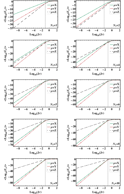
Figure 1: (color online) Single-axis errors after one cycle of $U_{\Omega}^{(N_{1},N_{2})}$ for outer sequence order $N_{2}=3$ and inner sequence orders $N_{1}=1,2,\ldots,10$ as a function of $J\tau$, averaged over $50$ random realizations of the bath operators $B_{\mu}$. Error bars are shown but are very small. In all our simulations we set $J=10^{-4}$ and $\beta=10^{-6}$. Single-axis error values were computed for $\log_{10}(J\tau)=-9,-8,\ldots,2$. Lines are guides to the eye. $E_{x}$ is the solid green line, $E_{y}$ is the dotted red line, and $E_{z}$ is the dashed black line. Note that $\log(E_{z})$ is the same in all six plots, with a slope of $N_{2}+1$. The slope of $\log(E_{x})$, on the other hand, is $N_{1}+1$. The slope of $\log(E_{y})$ is $N_{1}+2$. Vertical lines denote the largest value of $J\tau$ utilized in the linear regression used to extract the slope $n_{\mu}$.

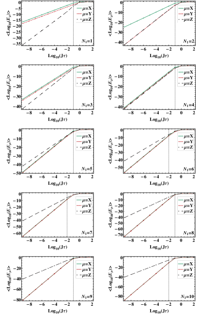
Figure 2: (color online) Single-axis errors after one cycle of $U_{\Omega}^{(N_{1},N_{2})}$ for outer sequence order $N_{2}=4$ and inner sequence orders $N_{1}=1,2,\ldots,10$ (left to right, top to bottom) as a function of $J\tau$, averaged over $50$ random realizations of the bath operators $B_{\mu}$. Other details as in Fig. 1, except that the single-axis error suppressed by both the inner and outer sequence, $E_{y}(\tau)$, exhibits a strong dependence on the parity of the inner sequence.

V.1 Single-axis errors

Figures 1 and 2 display the single-axis errors as a function of $J\tau$ for $N_{2}=3$ and $N_{2}=4$, respectively, with the inner sequence order varying from $N_{1}=1$ to $N_{1}=10$. The pure bath and system-bath interaction strengths were adjusted such that the Hamiltonian is dominated by the interaction, $\beta\ll J$. Each data point corresponds to a single cycle of the QDD sequence averaged over $50$ random instances of the parameters $c_{\alpha\beta}^{\mu}$ appearing in Eq. (28). Since we keep the minimum pulse interval fixed, the total sequence duration increases with increasing $N_{1}$ and $N_{2}$. The first thing to notice about Figures (1) and (2) is that they match the prediction of Eq. (32) very well in the regime of small $J\tau$. Namely, in all cases we observe a constant slope, until $J\tau\sim\mathcal{O}(1)$. This is also in agreement with the result of Ref. WFL:09 .

A summary of the scalings for $E_{\mu}(J\tau)$ are given in Table 1 for all combinations of $N_{1},N_{2}\in\{1,2,\ldots,10\}$. The values of $n_{\mu}$ were extracted by performing linear regressions for $\log_{10}[E_{\mu}(J\tau)]$ between $\log_{10}(J\tau)=-9$ and the values of $\log_{10}(J\tau)$ indicated by the vertical lines in Figs. 1 and 2, and rounding to the nearest integer (in all cases the deviation from an integer value was at most in the third significant digit). We shall return to Table 1 after presenting and discussing the data in the figures.

Let us then consider in detail the effect of varying the inner and outer sequence orders on the single-axis errors. When $N_{2}>N_{1}$, higher order suppression is expected for the errors that correspond to the system basis operators which anti-commute with the member of the MOOS comprising the outer $X$-type sequence. Thus the single-axis errors $E_{y}(\tau)$ and $E_{z}(\tau)$ are most heavily suppressed.

Since only the outer sequence can suppress $z$-axis, or $Z$-type errors [recall Eq. (5)], $E_{z}(J\tau)$ only gains additional error suppression if the outer sequence order is increased. In Fig. (1), $N_{2}=3$ and $E_{z}(J\tau)\sim\mathcal{O}[(J\tau)^{4}]$ for all $N_{1}$, exhibiting error suppression of the first $N_{2}$ terms of the interactions proportional to $\sigma^{z}$. Thus QDD operates with UDD efficiency for error suppression by the outer nested sequence alone.

In a similar manner to $E_{z}(J\tau)$, the behavior of $E_{x}(J\tau)$ can be attributed to one of the two nested sequences. Namely, the error measured by $E_{x}$ is associated with $\sigma^{x}$, which only anti-commutes with the MOOS operator present in the inner $Z$-type sequence. Determined solely by the inner sequence order, $E_{x}(J\tau)\sim\mathcal{O}[(J\tau)^{N_{1}+1}]$. Essentially, the outer sequence has no effect on the order of error suppression for $E_{x}(J\tau)$, as can be seen from Fig. 1 for $N_{2}=3$.

(a) $n_{x}=N_{1}+1$ for $N_{1},N_{2}\in\{1,\dots,10\}$
(b) $n_{y}$ $N_{1}$ $N_{2}=1$ $N_{2}=2$ $N_{2}=3$ $N_{2}=4$ $N_{2}=5$ $N_{2}=6$ $N_{2}=7$ $N_{2}=8$ $N_{2}=9$ $N_{2}=10$ 1 3 2 3 2 3 2 3 2 3 2 2 4 3 4 5 6 7 8 9 10 11 3 5 4 5 4 5 4 5 4 5 4 4 6 5 6 5 6 7 8 9 10 11 5 7 6 7 6 7 6 7 6 7 6 6 8 7 8 7 8 7 8 9 10 11 7 9 8 9 8 9 8 9 8 9 8 8 10 9 10 9 10 9 10 9 10 11 9 11 10 11 10 11 10 11 10 11 10 10 12 11 12 11 12 11 12 11 12 11
(c) $n_{z}$ $N_{1}$ $N_{2}=1$ $N_{2}=2$ $N_{2}=3$ $N_{2}=4$ $N_{2}=5$ $N_{2}=6$ $N_{2}=7$ $N_{2}=8$ $N_{2}=9$ $N_{2}=10$ 1 2 3 4 4 4 4 4 4 4 4 2 2 3 4 5 6 7 8 9 10 11 3 2 3 4 5 6 7 8 8 8 8 4 2 3 4 5 6 7 8 9 10 11 5 2 3 4 5 6 7 8 9 10 11 6 2 3 4 5 6 7 8 9 10 11 7 2 3 4 5 6 7 8 9 10 11 8 2 3 4 5 6 7 8 9 10 11 9 2 3 4 5 6 7 8 9 10 11 10 2 3 4 5 6 7 8 9 10 11

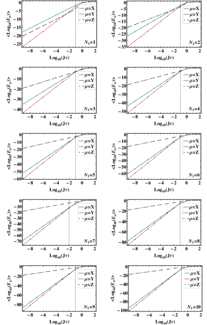
Figure 7: (color online) Single-axis errors after one cycle for $N_{2}=1$ and $N_{1}=1,2,\ldots,10$ (left to right, top to bottom). See Fig. 1 for additional details.

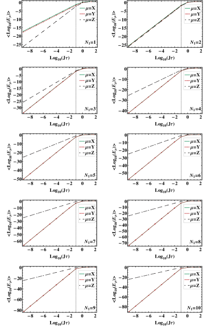
Figure 8: (color online) Single-axis errors after one cycle for $N_{2}=2$ and $N_{1}=1,2,\ldots,10$ (left to right, top to bottom). See Fig. 2 for additional details.

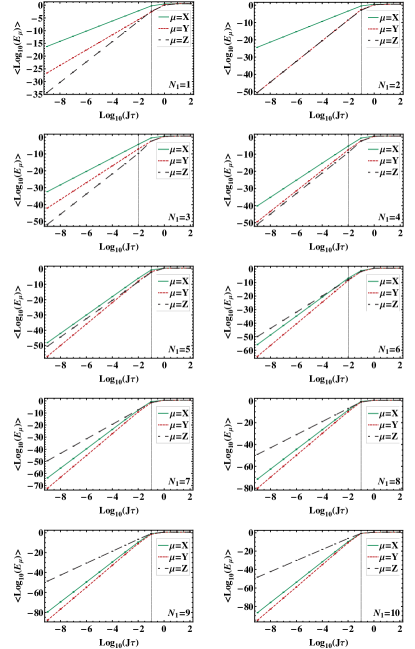
Figure 9: (color online) Single-axis errors after one cycle for $N_{2}=5$ and $N_{1}=1,2,\ldots,10$ (left to right, top to bottom). See Fig. 1 for additional details.

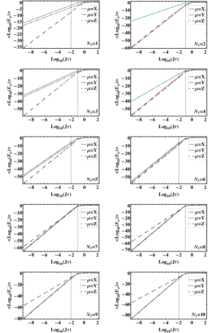
Figure 10: (color online) Single-axis errors after one cycle for $N_{2}=6$ and $N_{1}=1,2,\ldots,10$ (left to right, top to bottom). See Fig. 2 for additional details.

Table 1: Summary of the scaling for all single-axis errors. Values of $n_{\mu}$ were extracted by performing a linear regression, rounded to the nearest integer, fitting the slopes of the straight line portions of the curves displayed in Figs. 1 and 2, and the additional Figs. 7-10 in Appendix A, between $\log_{10}(J\tau)=-9$ and the values of $\log_{10}(J\tau)$ indicated by the vertical lines in these figures. (a) $E_{x}$, (b) $E_{y}$, and (c) $E_{z}$ for $N_{1},N_{2}\in\{1,2,\ldots,10\}$. For $n_{y}$ and $n_{z}$ the outer sequence order $N_{2}$ is displayed in the top row and the inner sequence order $N_{1}$ in the first column. Each of the single-axis errors is dominated by the lowest order of $J\tau$, denoted $n_{\mu}$, therefore $E_{\mu}\sim\mathcal{O}[(J\tau)^{n_{\mu}}]$. Additional simulations (not shown) fully continue the trends seen in this table and summarized in Eqs. (35)-(37) all the way up to $N_{1},N_{2}\leq 24$.

The interpretation for $E_{y}(J\tau)$ is not as simple, since this single-axis error is compensated by both the inner and outer sequences. One might expect both the inner and outer sequence to contribute to $Y$-type error suppression, i.e., $E_{y}(J\tau)$ to scale with $(J\tau)^{\max(N_{1},N_{2})+1}$. However, if this were the case then, e.g., the case $N_{1}=1$ would display an equal order of error suppression for both $E_{y}(\tau)$ and $E_{z}(\tau)$. Instead we find that $E_{y}(J\tau)\sim\mathcal{O}[(J\tau)^{N_{1}+2}]$ for $N_{2}=3$. Thus the suppression of $E_{y}(J\tau)$ is constrained by $N_{1}$, even when $N_{2}>N_{1}$, though it is larger by one order of magnitude than UDD error suppression efficiency for the inner sequence.

Similar observations apply for all odd-order outer sequences we have analyzed (see Appendix A, Figures 7 9, 11, and 13). Odd-order sequences are anti-symmetric with respect to time-reversal, and the conclusions concerning the case $N_{2}=3$ can be generalized as follows: when the outer sequence is anti-symmetric, terms in the QDD evolution operator which anti-commute with only one element of the MOOS are suppressed with UDD efficiency, determined by the order of the nested sequence composed of the corresponding anti-commuting MOOS operator (this applies to $\sigma^{x}$ and $\sigma^{z}$). In contrast, terma that anti-commutes with both elements of the MOOS are suppressed to one order beyond UDD efficiency, dictated exclusively by the inner sequence order (this applies to $\sigma^{y}$). Below we will see how this observation is modified when we consider larger values of $N_{2}$.

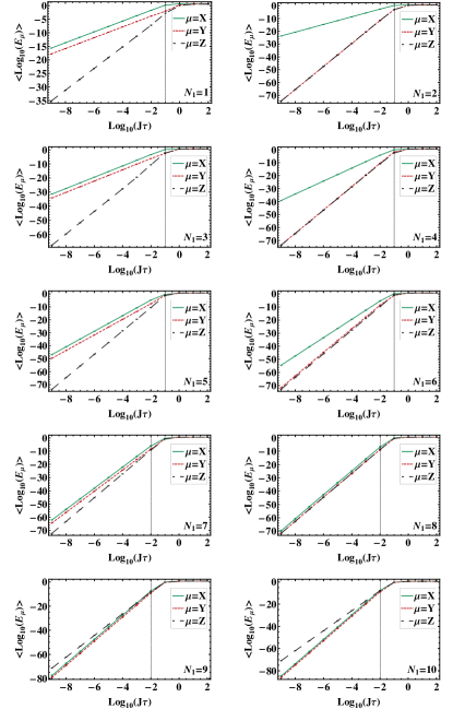
Figure 12: (color online) Single-axis errors after one cycle for $N_{2}=8$ and $N_{1}=1,2,\ldots,10$ (left to right, top to bottom). See Fig. 2 for additional details.

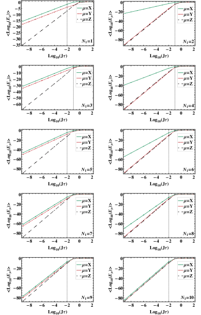
Figure 14: (color online) Single-axis errors after one cycle for $N_{2}=10$ and $N_{1}=1,2,\ldots,10$ (left to right, top to bottom). See Fig. 2 for additional details.

Comparing the case of the anti-symmetric outer sequence of Fig. 1 to that of the symmetric sequence of $N_{2}=4$ in Fig. 2, one notices immediately that there is a qualitative difference. The single-axis error $E_{y}(J\tau)$, the component anti-commuting with both the inner and outer sequences, $\sigma^{y}$, fluctuates strongly as a function of $N_{1}$. A similar effect is observed for other even values of $N_{2}$ (see Appendix A, Figures 8, 10, 12, and 14). Only the outer sequence order has been changed, therefore this characteristic is entirely dependent on the fact that the outer sequence is now symmetric.

Analogous to the anti-symmetric outer sequence, Fig. 2 shows that the single-axis error $E_{z}(J\tau)$ is independent of the inner sequence order. The scaling $E_{z}(J\tau)\sim\mathcal{O}[(J\tau)^{5}]$ holds for all $N_{1}$. Thus the single-axis error $E_{z}(J\tau)$ again exhibits UDD efficiency, independent of the parity of the outer sequence. Similarly, again $E_{x}(J\tau)\sim\mathcal{O}[(J\tau)^{N_{1}+1}]$ in Fig. 2.

However, when we consider the $n_{z}$ results for all values of $N_{1}$ and $N_{2}$ we find that there are exceptions to this simple behavior. As can be seen from Table 1, when $N_{1}=1$ and $N_{2}\geq 4$, the value of $n_{z}$ is fixed at $4$. The same phenomenon is observed for $N_{1}=3$ and $N_{2}\geq 8$.

On the basis of our numerical data we can summarize the scaling of the $X$ and $Z$-type single-axis errors as follows:

$$n_{x} = N_{1}+1,$$ (35)

and

$$n_{z}=\left\{\begin{array}[]{ll}N_{2}+1&:N_{1}\,\text{even}\\ N_{2}+1&:N_{1}\,\text{odd},\,N_{2}<2N_{1}+2\\ 2N_{1}+2&:N_{1}\,\text{odd},\,N_{2}\geq 2N_{1}+2\end{array}\right.$$ (36)

Qualitatively, we expect that when the inner sequence works imperfectly, as is the case for $N_{1}$ odd, the lowest order sequence will determine the scaling of the single axis error, and this is what is stated in Eq. (36).

As is clear from Fig. (2), the scaling of $E_{y}(J\tau)$ is dependent on the parity of $N_{1}$. If the inner sequence is of odd parity then $E_{y}(J\tau)\sim\mathcal{O}[(J\tau)^{N_{1}+2}]$ when $N_{2}$ is odd as well, or $E_{y}(J\tau)\sim\mathcal{O}[(J\tau)^{N_{1}+1}]$ when $N_{2}$ is even. Thus the scaling of $E_{y}$ is dominated by the inner sequence order when $N_{1}$ is odd. The situation changes when $N_{1}$ is even. Now, if $N_{2}$ is odd the sequence is still anti-symmetric, however there is an immediate improvement in error suppression, $E_{y}(J\tau)\sim\mathcal{O}[(J\tau)^{\max(N_{1}+1,N_{2})+1}]$. If the complete sequence is fully symmetric (both $N_{1}$ and $N_{2}$ even) we also find a scaling dependent on both the inner and outer sequence orders, $E_{y}(J\tau)\sim\mathcal{O}[(J\tau)^{\max(N_{1},N_{2})+1}]$. We thus see that the suppression of interactions which anti-commute with both elements of the MOOS depends sensitively on the parity of the inner sequence order, and is summarized for $E_{y}(J\tau)\sim\mathcal{O}[(J\tau)^{n_{y}}]$ as

$$n_{y}=\left\{\begin{array}[]{ll}\max(N_{1},N_{2})+1&:N_{1}\,\text{even},\,N_{2}\,\text{even}\\ \max(N_{1}+1,N_{2})+1&:N_{1}\,\text{even},\,N_{2}\,\text{odd}\\ N_{1}+1&:N_{1}\,\text{odd},\,N_{2}\,\text{even}\\ N_{1}+2&:N_{1}\,\text{odd},\,N_{2}\,\text{odd}\\ \end{array}\right.$$ (37)

The dependence upon the symmetry of the inner sequence, the parity of $N_{1}$, was first noted by Wang & Liu in the context of overall QDD performance NUDD . The dependence on the outer sequence symmetry, however, was not noted previously. Our results show that the symmetry of the outer sequence impacts the efficiency of $\sigma^{y}$ error suppression as well.

The efficiency of QDD error suppression is directly related to the efficiency of UDD. Each interaction that anti-commutes with at least one member of the MOOS is expected to achieve UDD efficiency. Fully symmetric QDD, i.e., even order $N_{1}$ and $N_{2}$, recovers the efficiency of UDD for all single-axis errors. Consequently, QDD performs with optimal efficiency when it is fully symmetric.

The interactions addressed only by the inner or outer sequence are separately suppressed with UDD efficiency corresponding to the order of the corresponding sequence performing the decoherence suppression. Equivalently, interactions which anti-commute with only one member of the MOOS are suppressed with UDD efficiency in the QDD scheme. On the other hand, error suppression of the interactions anti-commuting with both elements of the MOOS is dependent upon the parity of both the inner and outer sequence orders.

V.2 Intermediate single-axis errors

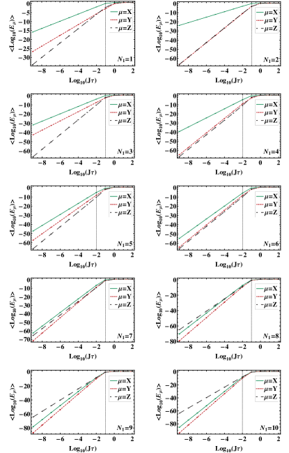
Figure 11: (color online) Single-axis errors after one cycle for $N_{2}=7$ and $N_{1}=1,2,\ldots,10$ (left to right, top to bottom). See Fig. 2 for additional details.

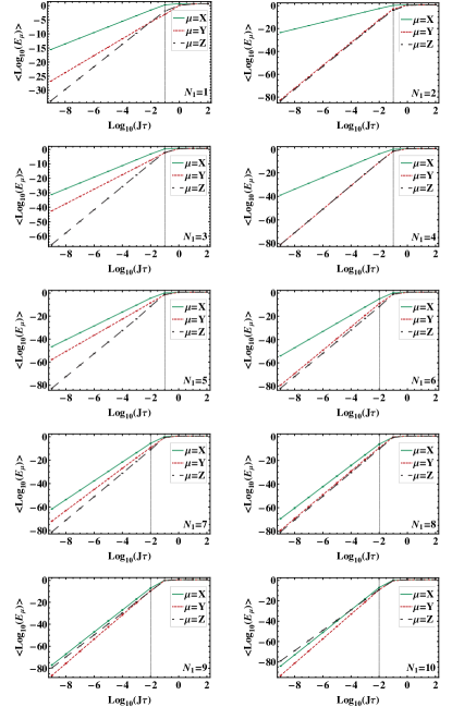
Figure 13: (color online) Single-axis errors after one cycle for $N_{2}=9$ and $N_{1}=1,2,\ldots,10$ (left to right, top to bottom). See Fig. 2 for additional details.

Rather than consider the single-axis errors just at the end of the QDD sequence, here we consider the single-axis errors prior to the application of each $X$-type outer sequence pulse. We will refer to these as “intermediate single-axis errors” since they are extracted during the QDD evolution, unlike those presented in Figures 1, 2, and 7-14 which are extracted at the end of the complete evolution. y studying this intermediate time-dependence of the errors we shall gain another interesting perspective on the manner in which the QDD sequence suppresses decoherence.

Let us define a set of “intermediate QDD” sequences as

$$\tilde{U}_{\Omega}^{(N_{1},j)}\equiv Z^{(N_{1})}(s_{j}\tau)XZ^{(N_{1})}(s_{j-1}\tau)\cdots XZ^{(N_{1})}(s_{1}\tau),$$ (38)

where $j\in\{1,\dots,N_{2}+1\}$. Thus, except for $j=1$, $\tilde{U}_{\Omega}^{(N_{1},j)}$ contains $j-1$ $X$-type pulses sandwiched between $j$ $Z$-type UDD sequences. When $j=1$

$$\tilde{U}_{\Omega}^{(N_{1},1)}\equiv Z^{(N_{1})}(s_{1}\tau)$$ (39)

is just the UDD sequence. We also separately define

$$\tilde{U}_{\Omega}^{(N_{1},N_{2}+2)}\equiv{U}_{\Omega}^{(N_{1},N_{2})}=X^{N_{2}}\tilde{U}_{\Omega}^{(N_{1},N_{2}+1)},$$ (40)

i.e., the complete QDD sequence, Eq. (5). Note that $\tilde{U}_{\Omega}^{(N_{1},N_{2}+2)}$ contains a final $X$ pulse if $N_{2}$ is odd, but not if $N_{2}$ is even. Similarly to the error expansion (21), we have the intermediate error expansion

$$\tilde{U}_{\Omega}^{(N_{1},j)}=B_{I}^{(j)}(\tau)+\sum_{\mu\in\{x,y,z\}}\sigma^{\mu}\otimes B_{\mu}^{(j)}(\tau).$$ (41)

In analogy to Eq. (22) we can now define the intermediate single-axis errors as

$$E_{\mu}^{(j)}(\tau)=\|B^{{(j)}}_{\mu}(\tau)\|_{F},$$ (42)

where $j\in\{1,N_{2}+2\}$. Note that for odd $N_{2}$ the errors $E_{\mu}^{(N_{2}+1)}$ and $E_{\mu}^{(N_{2}+2)}$ differ by a single instantaneous $X$ pulse (which is significant, as our simulations results will demonstrate), while for $N_{2}$ even $E_{\mu}^{(N_{2}+1)}=E_{\mu}^{(N_{2}+2)}$, so that below we do not plot $E_{\mu}^{(N_{2}+2)}$ in the even case.

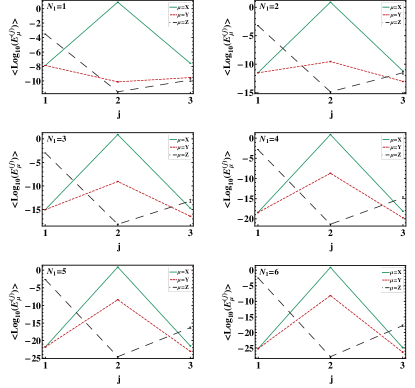
Figure 19: (color online) Intermediate single-axis errors for $N_{2}=1$. See Fig. 3 for additional details

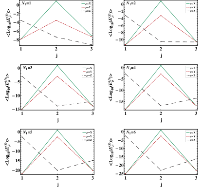
Figure 20: (color online) Intermediate single-axis errors for $N_{2}=2$. See Fig. 4 for additional details

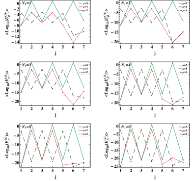
Figure 21: (color online) Intermediate single-axis errors for $N_{2}=5$. See Fig. 3 for additional details

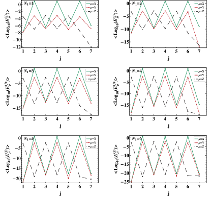
Figure 22: (color online) Intermediate single-axis errors for $N_{2}=6$. See Fig. 4 for additional details

Figures 3 and 4 display the intermediate single-axis errors for $N_{2}=3$ and $N_{2}=4$, respectively, with $N_{1}=1,2,\ldots,6$. The coupling parameters are fixed at $J=10^{-4}$ and $\beta=10^{-6}$ as in the previous figures. Additional results for odd $N_{2}$ are given in Appendix A in Figures 19 and 21, and for even $N_{2}$ in Appendix A in Figures 20 and 22.

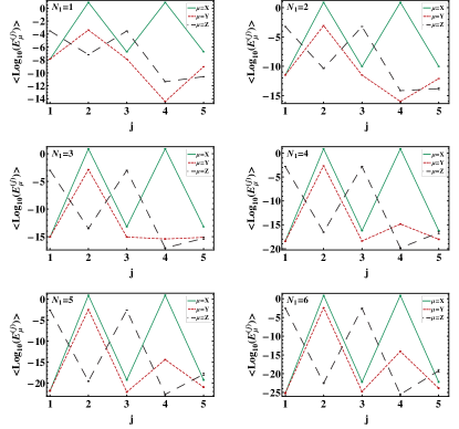
Figure 3: Intermediate single-axis errors for $N_{2}=3$, as defined in Eq. (42). For given $j$, the intermediate single-axis error is computed after $j$ innner $Z$-type UDD sequences separated by $j-1$ pulses. There are $N_{2}+1$ inner UDD sequences. The point $j=5$ is the last $X$ pulse at the end of last inner UDD sequence, as required for odd $N_{2}$. Note that because the data points labeled $j=4$ and $j=5$ are separated by a single $X$ pulse, and our pulses are instantaneous, these points have no actual time delay between them.

Several features are noteworthy in these figures.

(i) $E_{x}^{(1)}$ and $E_{y}^{(1)}$ are equal and substantially smaller than $E_{z}^{(1)}$, and the difference grows as $N_{1}$ is increased. This is because the inner $Z$-type sequence only suppresses the $X$ and $Y$-type errors, and the point $j=1$ does not include the first $X$-type outer sequence pulse. Formally, this is expressed by

$$E_{\mu}^{(1)}(\tau) = \|B^{{(1)}}_{\mu}\|_{F}\sim(s_{1}\tau)^{N_{1}+1},\quad\mu\in\{x,y\}$$

$$E_{\nu}^{(1)}(\tau) = \|B^{{(1)}}_{\nu}\|_{F}\sim 1,\quad\nu\in\{I,z\}.$$ (43)

(ii) The intermediate single-axis errors all fluctuate throughout the QDD evolution. This is due to a reshuffling of the errors after each outer sequence $X$-type pulse is applied, a simple consequence of the rules of Pauli matrix multiplication. To see why in some detail, consider the effect of the first $X\equiv\sigma^{x}\otimes I$ pulse:

$$X\tilde{U}_{\Omega}^{(N_{1},1)} = \sigma^{x}\otimes B_{I}^{(1)}+\sum_{\nu\in\{x,y,z\}}\sigma^{x}\sigma^{\nu}\otimes B_{\nu}^{(1)}$$

$$= B_{x}^{(1)}+\sigma^{x}\otimes B_{I}^{(1)}+\sigma^{y}\otimes B_{z}^{(1)}+\sigma^{z}\otimes B_{y}^{(1)},$$

where we dropped factors of $i$. The reshuffling effect is clear: for example, the error single-axis $z$-type error now comes from $B_{y}^{(1)}$. To explain the $j=2$ behavior we should consider the effect of multiplying $X\tilde{U}_{\Omega}^{(N_{1},1)}$ by the next inner UDD sequence $Z^{(N_{1})}(s_{2}\tau)$. The $i$th inner UDD sequence has the expansion

$$Z^{(N_{1})}(s_{i}\tau)=B_{I,i}+\sigma^{x}\otimes B_{x,i}+\sigma^{y}\otimes B_{y,i}+\sigma^{z}\otimes B_{z,i},$$ (45)

where similarly to Eq. (43) we have

$$\|B_{\mu,i}\|_{F} \sim (s_{i}\tau)^{N_{1}+1},\quad\mu\in\{x,y\}$$

$$\|B_{\nu,i}\|_{F} \sim 1,\quad\nu\in\{I,z\}.$$ (46)

Using this to carry out the multiplication to the next order we have

$$\tilde{U}_{\Omega}^{(N_{1},2)} = Z^{(N_{1})}(s_{2}\tau)X\tilde{U}_{\Omega}^{(N_{1},1)}$$

$$= [B_{I,2}+\sigma^{x}\otimes B_{x,2}+\sigma^{y}\otimes B_{y,2}+\sigma^{z}\otimes B_{z,2}]$$

$$\times [B_{x}^{(1)}+\sigma^{x}\otimes B_{I}^{(1)}+\sigma^{y}\otimes B_{z}^{(1)}+\sigma^{z}\otimes B_{y}^{(1)}]$$

Consequently

$$E_{x}^{(2)}(\tau)\!\! = \!\!\|B_{I,2}B_{I}^{(1)}+B_{x,2}B_{x}^{(1)}+B_{y,2}B_{y}^{(1)}+B_{z,2}B_{z}^{(1)}\|_{F}$$

$$\sim \!\!1$$

$$E_{y}^{(2)}(\tau)\!\! = \!\!\|B_{I,2}B_{z}^{(1)}+B_{x,2}B_{y}^{(1)}+B_{y,2}B_{x}^{(1)}+B_{z,2}B_{I}^{(1)}\|_{F}$$

$$\sim \!\!1$$

$$E_{z}^{(2)}(\tau)\!\! = \!\!\|B_{I,2}B_{y}^{(1)}+B_{x,2}B_{z}^{(1)}+B_{y,2}B_{I}^{(1)}+B_{z,2}B_{x}^{(1)}\|_{F}$$ (48)

$$\sim \!\!2(s_{1}\tau)^{N_{1}+1}+2(s_{2}\tau)^{N_{1}+1},$$

where $E_{x}^{(2)}(\tau)$ is dominated by $B_{I,2}B_{I}^{(1)}$ and $E_{y}^{(2)}(\tau)$ is dominated by $B_{I,2}B_{z}^{(1)}$, neither of which is suppressed, whence the $\sim 1$ result. On the other hand every one of the terms in $E_{z}^{(2)}(\tau)$ is suppressed. Hence, as can be seen in Figures 3 and 4 (and their companions, Figures 19-22 in the Appendix), at $j=2$ both the $X$ and $Y$-type errors have increased relative to $j=1$, while the $Z$-type error has decreased. One can similarly understand the remaining oscillations of the intermediate single-axis errors in terms of this reshuffling of error types.

(iii) $E_{x}$ and $E_{z}$ oscillate out of phase, while $E_{y}$ oscillates in phase with $E_{x}$ for even $N_{2}$, but not necessarily for odd $N_{1}$. This is again a consequence of error reshuffling. The $Y$-type error behaves differently from the other two since it experiences suppression from both the inner and outer sequences. For the same reason we always find $E_{y}^{(j)}<E_{x}^{(j)}$.

(iv) $E_{x}$ attains its minimum for $j=1$ and then slowly increases, though while maintaining its suppression order. This is because the $X$-type error is suppressed only by the inner sequences, and these are simply applied to it with fixed order ($N_{1}$), a total of $N_{2}$ or $N_{2}+1$ times. Repeated application of the inner UDD sequence is similar to the periodic DD (PDD) protocol, whose performance is well known to deteriorate as time grows KhodjastehLidar:07 ; KhodjastehLidar:08 . The reason is that the error accumulates over time, without a mechanism for reducing it.

(v) There does not appear to be much of a difference between even and odd values of $N_{2}$ in terms of the intermediate single-axis errors. One difference is that $E_{y}^{(j)}$ tends to be more erratic for odd $N_{2}$ at high $j$ values. We do not have a simple explanation for this behavior. Another difference is that for even $N_{2}$ all single-axis errors have the same final value when $N_{1}=N_{2}$, but for odd $N_{2}$ the $X$-type error is always slightly worse at the end of the sequence, thus setting the bottleneck. Perhaps additional pulse interval optimization can remove this asymmetry.

(vi) Only at the very end are all three single-axis errors simultaneously small. Thus, while suppression of one error type can be achieved in the middle of the QDD sequence, one must wait until its completion to suppress all errors.

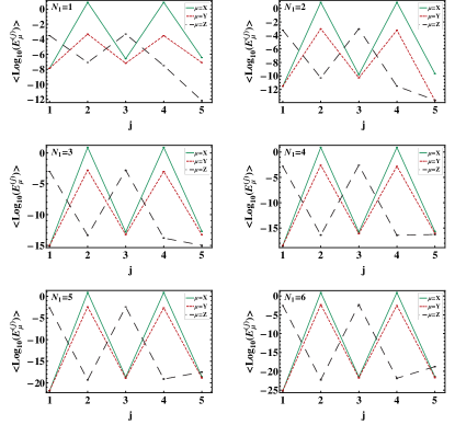
Figure 4: (color online) Intermediate single-axis errors for $N_{2}=4$. As in Fig. 3 except that there is no final $X$ pulse for $N_{2}$ even, i.e., there are $N_{2}+1$ inner UDD sequences separated by $N_{2}$ $X$ pulses.

V.3 Overall performance

$n_{D}$
$N_{1}$	$N_{2}=1$	$N_{2}=2$	$N_{2}=3$	$N_{2}=4$	$N_{2}=5$	$N_{2}=6$	$N_{2}=7$	$N_{2}=8$	$N_{2}=9$	$N_{2}=10$
1	2	2	2	2	2	2	2	2	2	2
2	2	3	3	3	3	3	3	3	3	3
3	2	3	4	4	4	4	4	4	4	4
4	2	3	4	5	5	5	5	5	5	5
5	2	3	4	5	6	6	6	6	6	6
6	2	3	4	5	6	7	7	7	7	7
7	2	3	4	5	6	7	8	8	8	8
8	2	3	4	5	6	7	8	9	9	9
9	2	3	4	5	6	7	8	9	10	10
10	2	3	4	5	6	7	8	9	10	11

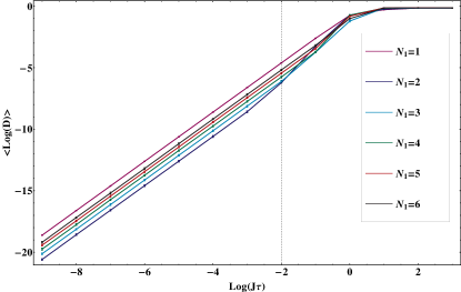
Figure 15: (color online) Overall QDD distance measure after one cycle for $N_{2}=1$ and $N_{1}=1,2,\ldots,6$ (left to right, top to bottom). See Fig. 5 for additional details.

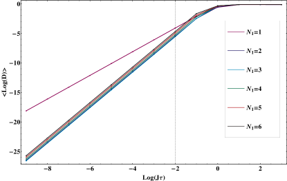
Figure 16: (color online) Overall QDD distance measure after one cycle for $N_{2}=2$ and $N_{1}=1,2,\ldots,6$ (left to right, top to bottom). See Fig. 6 for additional details.

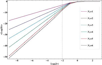
Figure 17: (color online) Overall QDD distance measure after one cycle for $N_{2}=5$ and $N_{1}=1,2,\ldots,6$ (left to right, top to bottom). See Fig. 5 for additional details.

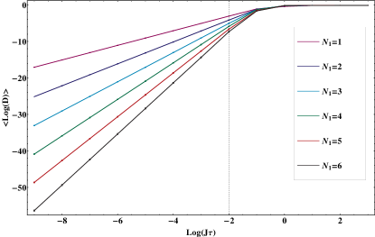
Figure 18: (color online) Overall QDD distance measure after one cycle for $N_{2}=6$ and $N_{1}=1,2,\ldots,6$ (left to right, top to bottom). See Fig. 6 for additional details.

Table 2: Summary of the scaling of the overall distance measure $D$ with respect to inner and outer sequence orders, $N_{1}$ and $N_{2}$, respectively. Values of $n_{D}$ were extracted by performing a linear regression, rounded to the nearest integer, fitting the slopes of the straight line portions of the curves displayed in Figs. 1 and 2 and the additional Figs. 15-18 in Appendix A between $\log(J\tau)=-9$ and the values of $\log(J\tau)$ indicated by the vertical lines in these figures. The outer sequence order $N_{2}$ is displayed in the top row and the inner sequence order $N_{1}$ in the first column. We find that, as expected, $n_{D}=\min(n_{x},n_{y},n_{z})$. Additional simulations (not shown) fully continue the trends seen in this table and summarized in Eq. (50) all the way up to $N_{1},N_{2}\leq 24$.

While the single-axis error analysis presented in the previuous two subsections helps in unravelling the mechanism of QDD performance, it does of course not tell the whole story. We now present our results for the distance measure $D(U,I)$ [Eq. (25)], which provides a complete quantitative description of QDD performance. We expect this overall performance of QDD to be dictated by the lowest order of $\tau$ present in the final evolution operator, Eq. (21), i.e.,

$$D\sim\mathcal{O}[(J\tau)^{n_{D}}]$$ (49)

where

$$n_{D}=\min(n_{x},n_{y},n_{z}).$$ (50)

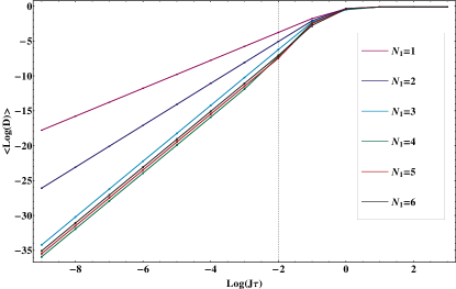
Figure 5: (color online) Overall QDD distance measure after one cycle of $U_{\Omega}^{(N_{1},N_{2})}$ for outer sequence order $N_{2}=3$ and inner sequence orders $N_{1}=1,2,\ldots,6$, as a function of $J\tau$, averaged over $50$ random realizations of the bath operators $B_{\mu}$. The performance of QDD progressively improves with increasing $N_{1}$ up to $N_{2}=N_{1}$, indicating that $\min\{N_{1},N_{2}\}$ dominates QDD performance.

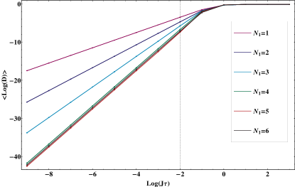
Figure 6: (color online) Overall QDD distance measure after one cycle of $U_{\Omega}^{(N_{1},N_{2})}$ for outer sequence order $N_{2}=4$ and inner sequence orders $N_{1}=1,2,\ldots,6$, as a function of $J\tau$, averaged over $50$ random realizations of the bath operators $B_{\mu}$. The dependence of the order of error suppression on $\min\{N_{1},N_{2}\}$ is again observed.

Overall QDD performance for $N_{2}=3$ and $N_{2}=4$ is shown in Figures 5 and 6, respectively. The outer sequence order $N_{2}$ is fixed and the inner sequence order $N_{1}$ is varied from $1$ to $6$. These results are for the same model considered in the previous subsection. Additional results are given in Appendix A for $N_{2}=1,2,5,6$ (see Figures 15-18). A summary of the distance scaling results is presented in Table 2.

Considering $N_{2}=3$ first (Fig. 5), when $N_{2}>N_{1}$ the overall order of error suppression is hindered by the inner sequence order. This is evident by the increasing order of error suppression as $N_{1}$ increases. In this regime the lower sequence order is determined by the inner sequence, therefore the scaling of $D$ is equivalent to that of $E_{x}$, i.e., $D\sim\mathcal{O}[(J\tau)^{N_{1}+1}]$. As $N_{1}$ passes $N_{2}$, there is a saturation of error suppression corresponding to a performance bounded by the lower outer sequence order. The amplitude of performance increases slightly beyond $N_{2}=N_{1}$, however begins to decrease when $N_{1}>N_{2}$, as evidenced not by the slope but by the offset of the distance curves. Namely, the ordering, from worst to best, is $N_{1}=6,5,4$. The latter is an interesting feature not easily deduced from the single-axis errors. Increasing the inner sequence order results in an accumulation of error for the single-axis error dominating the performance; when $N_{1}>N_{2}+1$ this corresponds to $E_{z}$.

The results are similar for $N_{2}=4$, as shown by Fig. 6. The order of error suppression, given by the slope, increases until $N_{1}=N_{2}$ in correspondence with an overall performance dominated by the lowest order of $\tau$ present in $E_{\mu}$. In addition to the saturation of the order of error suppression, we again observe an offset-related deterioration. Namely, $N_{1}=6$ is slightly worse than $N_{1}=5$.

VI Conclusions

This work presents a comprehensive numerical analysis of the error suppression characteristics of QDD. This was achieved by isolating the single-axis errors associated with each system basis operator in the system-bath interaction. The order of error suppression was determined by computing the single-axis error as a function of the minimum pulse interval. We performed our analysis for a model in which the system-environment interaction dominated the internal bath dynamics, so that we could study the properties of the single-axis errors in the regime where DD is most beneficial. We constructed our QDD sequences with $N_{1}$ $Z$-type pulses comprising the inner sequence, and $N_{2}$ $X$-type pulses comprising the outer sequence. We found that the system-bath interaction term proportional to $\sigma^{x}$ is suppressed with UDD efficiency for all values of $N_{1}$ and $N_{2}$ [Eq. (35)]. The interactions proportional to $\sigma^{z}$ and $\sigma^{y}$ both exhibit parity effects [Eqs. (36), (37)] whose origins are the symmetry or anti-symmetry of the inner and outer UDD sequences. Of course, permuting the pulse types of the inner and outer sequences will correspondingly modify these conclusions.

We also performed an analysis of the intermediate time-dependent performance of QDD. We found that the single-axis errors are strongly time-dependent, oscillating between outer-sequence pulses, until they all converge to nearly the same value after the final outer-sequence pulse. The closest convergence occurs for QDD sequences with equal inner and outer orders.

Finally, we computed the overall performance of QDD using an appropriate distance measure, and reconciled its scaling with that of the single-axis errors. We showed that overall QDD error suppression scales with the lowest order of single-axis error suppression, i.e., the first non-vanishing contribution appears at order $\min(N_{1},N_{2})+1$. QDD accomplishes this by applying $(N_{1}+1)(N_{2}+1)$ pulses. We conjecture that similarly, for NUDD with $K$ nested UDD sequences using $(N_{1}+1)(N_{2}+1)\cdots(N_{K}+1)$ pulses, the first non-vanishing contribution will appear at order $\min_{j}(N_{j})+1$.

In this work we treated the pulses as ideal, instantaneous operations. However, this is of course an idealization. An important topic for future study is robustness with respect to pulse errors, whether random or systematic. This topic has been addressed for UDD both theoretically Uhrig:09a ; Pasini:10 and experimentally PhysRevA.83.032303 , and the overall conclusion is that pulse errors can have a dramatic negative impact unless they are compensated for. Some combination of pulse shaping and optimization will surely be required to overcome this problem in the context of QDD as well.

Appendix A Additional Numerical Results

In this appendix we present additional figures in support of the numerical results presented in the body of the paper.