Multichannel Quantum Defect Theory for cold molecular collisions

Abstract

Multichannel Quantum Defect Theory (MQDT) is shown to be capable of producing quantitatively accurate results for low-energy atom-molecule scattering calculations. With a suitable choice of reference potential and short-range matching distance, it is possible to define a matrix that encapsulates the short-range collision dynamics and is only weakly dependent on energy and magnetic field. Once this has been produced, calculations at additional energies and fields can be performed at a computational cost that is proportional to the number of channels $N$ and not to $N^{3}$. MQDT thus provides a promising method for carrying out low-energy molecular scattering calculations on systems where full exploration of the energy- and field-dependence is currently impractical.

Note for copy editor: We have been very careful to make correct use of Roman and italic subscripts and superscripts, with Roman for abbreviations and italic for mathematical indices. Please do not change all our subscripts and superscripts to italic. Also note that subscript lower-case o is an abbreviation for “open” and should not be changed to zero.

I Introduction

The creation of the first dilute atomic Bose-Einstein condensates (BECs) in 1995 Anderson et al. (1995); Davis et al. (1995) led to enormous advances in ultracold atomic physics. There is now great interest in producing samples of cold molecules, at temperatures below 1 K Doyle et al. (2004); Krems (2005); Friedrich and Doyle (2009), and ultracold molecules, at temperatures below 1 mK Hutson and Soldán (2006); Ni et al. (2008); Ospelkaus et al. (2010); Danzl et al. (2010). There are many potential applications of ultracold molecular samples, amongst which are high-precision measurements Hudson et al. (2002); Bethlem and Ubachs (2009), quantum computation DeMille (2002) and ultracold chemistry Bell and P. Softley (2009).

Understanding atomic and molecular interactions and collisions is essential to the study of cold and ultracold molecules. For example, methods such as buffer-gas cooling Weinstein et al. (1998) and Stark deceleration Bethlem and Meijer (2003) can produce cold molecules with temperatures between 10 mK and 1 K. However, a second-stage cooling method is needed to bring the molecules into the ultracold regime. Sympathetic cooling, in which the molecules are allowed to thermalize with a gas of ultracold atoms, is a promising second-stage cooling method Soldán and Hutson (2004). However, while elastic collisions allow thermalization, inelastic collisions can cause trap loss deCarvalho et al. (1999), and for many systems the inelastic collisions are predicted to be too large for sympathetic cooling to succeed Lara et al. (2007); Żuchowski and Hutson (2009); Tokunaga et al. (2011). Scattering calculations are essential in order to identify systems for which sympathetic cooling has a good prospect of success. Once in the ultracold regime, the extent to which atomic and molecular interactions can be controlled again depends on a detailed understanding of their collisional properties.

Quantum molecular scattering calculations are usually carried out using the coupled-channel method: the Schrödinger equation for scattering is converted into a set of coupled differential equations, which are then propagated across a range of values of the intermolecular distance $r$. The size of the problem is determined by the number of channels $N$ (the number of coupled equations). The usual algorithms take a time proportional to $N^{3}$, since each step of the propagation requires an $\mathcal{O}(N^{3})$ matrix operation.

Cold molecule scattering presents problems with a large number of channels for two reasons:

1. At very low energies, small splittings between molecular energy levels become important. This makes it necessary to include fine details of molecular energy level patterns, such as tunneling and nuclear hyperfine splitting. The extra degrees of freedom require additional basis functions; in particular, including nuclear spins can multiply the number of equations by a substantial factor (sometimes 100 or more).

2. Collisions in the presence of electric and magnetic fields are very important. In an applied field, the total angular momentum $J$ is no longer a good quantum number. Because of this, the large sets of coupled equations can no longer be factorized neatly into smaller blocks for each $J$ as is possible in field-free scattering.

In addition, in cold molecule applications it is often necessary to repeat scattering calculations on a fine grid of energies and/or applied electric and magnetic fields, which adds greatly to the computational expense.

Multichannel Quantum Defect Theory (MQDT) offers an alternative to full coupled-channel calculations. It was originally developed to provide a uniform treatment of bound and scattering states for problems involving the interaction an electron with an ion core with Coulomb forces at long range Seaton (1966, 1983), but was subsequently generalized to handle a range of other long-range potentials Greene et al. (1979, 1982); Seaton (1983); Mies (1984); Yoo and Greene (1986); Gao (2008). It has been successfully applied to scattering problems as diverse as negative ion photodetachment Watanabe and Greene (1980), near-threshold predissociation of diatomic molecules Mies (1984); Mies and Julienne (1984) and predissociation of atom-diatom Van der Waals complexes Raoult and Balint-Kurti (1988, 1990). More recently it has been applied to ultracold collisions between pairs of neutral atoms Julienne and Mies (1989); Burke et al. (1998); Mies and Raoult (2000); Raoult and Mies (2004); Gao et al. (2005), between atoms and ions Idziaszek et al. (2009); Gao (2010a), and between highly reactive molecules Idziaszek and Julienne (2010); Idziaszek et al. (2010); Gao (2010b).

MQDT can be viewed in two different ways. The first tries to capture the important physics of collisions within a few analytic quantum defect parameters. The other views it as a method for solving the coupled equations of scattering theory which offers substantial insights and advantages in efficiency. The common feature of the two approaches is to take advantage of the enormous difference in energy and length scales associated with separated collision partners and short-range potentials.

When MQDT is viewed as a numerical method for solving the coupled differential equations, the goal is to obtain a matrix $\bm{Y}(E,B)$ Greene et al. (1982); Mies and Julienne (1984); Mies and Raoult (2000); Raoult and Mies (2004) that completely describes the short-range dynamics and is insensitive to collision energy $E$ and magnetic field $B$. This matrix can be obtained once and then used for calculations over a wide range of energies and fields, or obtained by interpolation from a few points. MQDT achieves this by defining $\bm{Y}(E,B)$ at relatively short range, as described below. The threshold behavior is accounted for from properties of single channels. Once the matrix $\bm{Y}(E,B)$ has been obtained, the time required for calculations at additional energies and fields is only proportional to $N$, not $N^{3}$.

Understanding threshold atomic physics in quantum defect terms is well developed Julienne and Mies (1989); Burke et al. (1998); Mies and Raoult (2000); Vogels et al. (2000); Gao (2001). Threshold bound-state and scattering properties are determined mainly by the long-range potential, which can often be approximated as $-C_{n}/r^{n}$. For the case of the Van der Waals interaction, $-C_{6}/r^{6}$, the linearly independent pair of solutions for a single potential is known Gao (1998a). An analytic approach to MQDT using these solutions has been developed Gao (1998b, 2009) and gives much insight into ultracold atom-atom collisions Julienne and Gao (2006).

This paper investigates the use of MQDT as a numerical method to study cold atom-molecule collisions. The structure of the paper is as follows. In Section II we give an overview of the theory of MQDT, sufficient to define notation. In Section III we apply MQDT to the prototype system Mg+NH, and compare it with full coupled-channel calculations in order to establish what is required for it to give accurate results. In Section IV we present our conclusions and suggest directions for future work.

II Theory

II.1 Coupled-channel method

Cold atomic and molecular collisions and near-threshold bound states are conveniently described by a set of coupled equations. The Hamiltonian for an interacting pair of atoms or molecules is of the form

$$-\frac{\hbar^{2}}{2\mu}\nabla^{2}+\hat{H}_{\text{int}}(\tau)+V(r,\tau),$$ (1)

where $\mu$ is the reduced mass, $\nabla^{2}$ is the Laplacian for the intermolecular coordinates, and $\tau$ denotes all coordinates except the interparticle distance $r$. $\hat{H}_{\text{int}}(\tau)$ represents the internal Hamiltonians of the two particles and $V(r,\tau)$ is the interaction potential. The total wavefunction is expanded

$$\Psi(r,\tau)=r^{-1}\sum_{i}\varphi_{i}(\tau)\psi_{i}(r),$$ (2)

where the $N$ functions $\varphi_{i}(\tau)$ form a basis set for the motion in all coordinates, $\tau$, except the intermolecular distance, and $\psi_{i}(r)$ is the radial wavefunction in channel $i$. Substituting this expansion into the total time-independent Schrödinger equation and projecting onto the basis function $\varphi_{j}(\tau)$ yields the usual coupled equations of scattering theory,

$$\left[-\frac{\hbar^{2}}{2\mu}\frac{d^{2}}{dr^{2}}-E\right]\psi_{j}(r)=-\sum_{i}W_{ji}(r)\psi_{i}(r),$$ (3)

where $E$ is the energy. The coupling matrix $\bm{W}$ has elements

$$W_{ji}(r)=\int\varphi_{j}^{*}(\tau) \bigg{[}H_{\text{int}}(\tau)+V(r,\tau)$$ (4)

$$\quad+\ \frac{\hbar^{2}L_{i}(L_{i}+1)}{2\mu r^{2}}\bigg{]}\varphi_{i}(\tau)\,d\tau,$$

where $L_{i}$ is the partial-wave quantum number for channel $i$. Equation (3) can conveniently be written in matrix form,

$$\frac{\hbar^{2}}{2\mu}\frac{d^{2}\bm{\psi}}{dr^{2}}=[\bm{W}(r)-E\bm{I}]\bm{\psi}(r),$$ (5)

where $\bm{\psi}(r)$ is a column vector made up of the solutions $\psi_{i}(r)$ and $\bm{I}$ is the identity matrix.

For both bound states and collision calculations, the wavefunction must be regular at the origin. When $V(r)\gg 0$ as $r\rightarrow 0$, the short-range boundary condition is

$$\psi_{i}(r)\rightarrow 0\text{\quad as\quad}r\rightarrow 0.$$ (6)

At any energy, there are $N$ linearly independent solution vectors $\bm{\psi}(r)$ that satisfy these boundary conditions, and it is convenient to combine them to form the $N\times N$ wavefunction matrix $\bm{\Psi}$(r).

The coupled-channel approach propagates either the wavefunction matrix $\bm{\Psi}(r)$ and its derivative $\bm{\Psi}^{\prime}(r)$, or the log-derivative matrix $\bm{L}(r)=\bm{\Psi}^{\prime}[\bm{\Psi}]^{-1}$, outwards from $r=0$ (or a point in the deeply classically forbidden region at short range) Gordon (1969); Johnson (1973). In scattering calculations, the propagation is continued to a point $r_{\text{max}}$ at large $r$. The wavefunction or log-derivative matrix is then transformed into a representation where $\bm{W}$ is asymptotically diagonal González-Martínez and Hutson (2007), such that

$$W_{ji}(r)\stackrel{{\scriptstyle r\rightarrow\infty}}{{\longrightarrow}}\left[E_{i}^{\infty}+\frac{\hbar^{2}L_{i}(L_{i}+1)}{2\mu r^{2}}\right]\delta_{ij}+\mathcal{O}(r^{-n}),$$ (7)

where $n$ is the power of the leading term in the potential expansion and $E_{i}^{\infty}$ is the threshold of channel $i$. Each channel is either asymptotically open, $E\geq E_{i}^{\infty}$, or asymptotically closed, $E<E_{i}^{\infty}$. The scattering boundary conditions are

$$\bm{\Psi}=\bm{J}(r)+\bm{N}(r)\bm{K}.$$ (8)

The matrices $\bm{J}$ and $\bm{N}$ are diagonal matrices containing Riccati-Bessel functions for open channels and modified spherical Bessel functions for closed channels Johnson (1973). In a problem containing $N$ channels, $N_{\text{o}}$ of which are open, the scattering $\bm{S}$ matrix is related to the open-open submatrix of $\bm{K}$ by

$$\bm{S}=(1+i\bm{K}_{\text{oo}})^{-1}(1-i\bm{K}_{\text{oo}}).$$ (9)

In full coupled-channel calculations, the matrices $\bm{K}$ and $\bm{S}$ are rapidly changing functions of both energy and field, particularly near scattering resonances, so that the entire propagation to long range must be repeated for each set of conditions required.

II.2 Multichannel Quantum Defect Theory

MQDT also begins by propagating the wavefunction or log-derivative matrix outwards from short range. However, instead of continuing to $r_{\text{max}}$, matching takes place at a point $r_{\text{match}}$, at relatively short range. The matching in MQDT treats the open and weakly closed channels on an equal footing; weakly closed channels are usually defined as those that are locally open, $E>W_{ii}(r)$, at some value of $r$, so are capable of supporting scattering resonances. Matching at short range produces a matrix $\bm{Y}(E,B)$ that is relatively insensitive to energy and applied field, as described below. $\bm{Y}$ also varies smoothly across thresholds, unlike $\bm{S}$ and $\bm{K}$. Provided the channels are uncoupled outside $r_{\text{match}}$, it is then possible to obtain the scattering $\bm{S}$ matrix from $\bm{Y}$ using the properties of individual uncoupled channels.

We consider a problem with $N_{\text{o}}$ open channels and $N_{\text{c}}$ weakly closed channels at some collision energy $E$ and field $B$. For each such channel, $i=1,N$, where $N=N_{\text{o}}+N_{\text{c}}$, MQDT requires a reference potential, $U_{i}^{\text{ref}}(r)$, which asymptotically has similar behavior to $W_{ii}(r)$ in equation (7). This reference potential defines a linearly independent pair of reference functions $f_{i}(r)$ and $g_{i}(r)$,

$$\left[\frac{d^{2}}{dr^{2}}+K^{2}_{i}(r)\right]f_{i}(r)=0,$$ (10)

and similarly for $g_{i}$, where the local wave vector $K_{i}(r)$ is

$$K_{i}(r)=\sqrt{\frac{2\mu}{\hbar^{2}}(E-U^{\text{ref}}_{i}(r))}.$$ (11)

The regular solution $f_{i}$ has the boundary condition $f_{i}\rightarrow 0$ as $r\rightarrow 0$. $f_{i}$ and $g_{i}$ are normalized to have Wentzel-Kramers-Brillouin (WKB) form, with amplitude $K_{i}(r)^{-1/2}$, at some point in the classically allowed region Greene et al. (1982). The $N\times N$ matrix $\bm{Y}$ is defined by matching at $r_{\text{match}}$,

$$\bm{\Psi}=\bm{f}(r)+\bm{g}(r)\bm{Y},$$ (12)

or in terms of the log-derivative matrix $\bm{L}$,

$$(\bm{Lf}-\bm{f}^{\prime})=(\bm{Lg}-\bm{g^{\prime}})\bm{Y},$$ (13)

where $\bm{f}$ and $\bm{g}$ are diagonal matrices containing the functions $f_{i}$ and $g_{i}$ and the primes indicate radial derivatives.

In order to relate $\bm{Y}$ to the physical scattering $\bm{S}$ matrix, the asymptotic forms of the reference functions $f_{i}$ and $g_{i}$ in each channel are required. To this end another pair of reference functions is defined for each channel. For open channels, these functions are asymptotically energy-normalized,

$$s_{i}(r)\stackrel{{\scriptstyle r\rightarrow\infty}}{{\longrightarrow}}k_{i}^{-\frac{1}{2}}\sin{\left(k_{i}r-\frac{L_{i}\pi}{2}+\xi_{i}\right)},$$ (14)

$$c_{i}(r)\stackrel{{\scriptstyle r\rightarrow\infty}}{{\longrightarrow}}k_{i}^{-\frac{1}{2}}\cos{\left(k_{i}r-\frac{L_{i}\pi}{2}+\xi_{i}\right)},$$ (15)

where $\xi_{i}$ is the phase shift associated with reference potential $i$ and $k_{i}$ is the asymptotic wave vector,

$$k_{i}=\sqrt{\frac{2\mu}{\hbar^{2}}(E-E_{i}^{\infty})}.$$ (16)

These asymptotically normalized functions are related to $f_{i}$ and $g_{i}$ through the quantum defect parameters $C_{i}$ and $\tan\lambda_{i}$,

$$s_{i}(r) = C_{i}^{-1}f_{i}(r);$$ (17)

$$c_{i}(r) = C_{i}[g_{i}(r)+\tan\lambda_{i}f_{i}(r)].$$ (18)

Thus $C_{i}$ relates the amplitudes of the energy-normalised reference functions to WKB-normalised ones, while $\tan\lambda_{i}$ describes the modification in phase due to threshold effects. Far from threshold, $C_{i}\approx 1$ and $\tan\lambda_{i}\approx 0$.

For each weakly closed channel, an exponentially decaying solution is defined,

$$\phi_{i}(r)\stackrel{{\scriptstyle r\rightarrow\infty}}{{\longrightarrow}}\textstyle{\frac{1}{2}}e^{-|k_{i}|r}\sqrt{|k_{i}|}.$$ (19)

This is related to the solutions $f_{i}$ and $g_{i}$ by a normalization factor $\mathcal{N}_{i}$, and an energy-dependent phase $\nu_{i}$,

$$\phi_{i}(r)=\mathcal{N}_{i}\left[\cos{\nu}_{i}f_{i}(r)-\sin{\nu}_{i}g_{i}(r)\right].$$ (20)

The phase $\nu_{i}$ is an integer multiple of $\pi$ at each energy that corresponds to a bound state of the reference potential in channel $i$.

The $\bm{Y}$ matrix is converted into the $\bm{S}$ matrix of scattering theory using the quantum defect parameters $C_{i}$, $\tan\lambda_{i}$, $\tan\nu_{i}$ and $\xi_{i}$. First, the effect of coupling to closed channels is accounted for,

$$\bm{\overline{Y}}=\bm{Y}_{\text{oo}}-\bm{Y}_{\text{oc}}[\tan\bm{\nu}+\bm{Y}_{\text{cc}}]^{-1}\bm{Y}_{\text{co}},$$ (21)

where $\tan\bm{\nu}$ is a diagonal matrix of dimension $N_{\text{c}}\times N_{\text{c}}$ containing elements $\tan\nu_{i}$. The $N_{\text{o}}\times N_{\text{o}}$ matrix $\bm{\overline{Y}}$ incorporates any resonance structure caused by coupling to closed channels through $\tan\bm{\nu}$. Unlike $\bm{Y}$ itself, $\bm{\overline{Y}}$ can be a rapidly varying function of energy and field. Secondly, threshold effects from asymptotically open channels are incorporated,

$$\bm{\overline{R}}=\bm{C}^{-1}\left[\bm{\overline{Y}}^{-1}-\tan\bm{\lambda}\right]^{-1}\bm{C}^{-1},$$ (22)

where $\bm{C}$ and $\tan\bm{\lambda}$ are diagonal matrices of dimension $N_{\text{o}}\times N_{\text{o}}$, containing elements $C_{i}$ and $\tan\lambda_{i}$. Finally, the $\bm{S}$ matrix is obtained from

$$\bm{S}=e^{i\bm{\xi}}\left[1+i\bm{\overline{R}}\right]\left[1-i\bm{\overline{R}}\right]^{-1}e^{i\bm{\xi}}.$$ (23)

This may be compared to equation (9) for the full coupled-channel method. The inclusion of the diagonal matrix $e^{i\bm{\xi}}$ accounts for the phase difference between the reference functions $f_{i}$ and $g_{i}$ used by MQDT and the Riccati-Bessel functions used by the full coupled-channel method.

The approach taken in the present paper is somewhat different from that in refs. Mies (1984); Mies and Raoult (2000). There MQDT was approached as an exact representation of the full coupled-channel solution. The matrix $\bm{Y}$ was evaluated at a distance $r_{\text{match}}$ large enough that it had become constant as a function of $r_{\text{match}}$. When this is done, MQDT gives the same (exact) results for any choice of reference potential $U^{\rm ref}_{i}(r)$, although constancy of $\bm{Y}$ may be achieved at different values of $r_{\text{match}}$ for different choices. In our approach, $r_{\text{match}}$ is chosen to ensure that $\bm{Y}$ is only weakly energy-dependent, and this may require matching in a region where $\bm{Y}$ is not yet independent of $r_{\text{match}}$. With this approach, MQDT provides an approximate solution whose quality depends on the choice of reference potentials.

II.3 Numerical evaluation of reference functions and quantum defect parameters

II.3.1 Open channels

For an open channel $i$, the reference function $s_{i}$ is obtained by propagating a regular solution of (10) from a point inside $r_{\text{match}}$ to a point $r_{\text{max}}$ at long range and imposing the boundary condition (14) (or its Bessel function equivalent). This establishes the normalization of $s_{i}$ and also gives the phase shift $\xi_{i}$, which is then used to obtain the function $c_{i}$ at $r_{\text{max}}$ from the boundary condition (15). The reference function $c_{i}$ is then propagated inwards to $r_{\text{match}}$. The two remaining quantum defect parameters are obtained by applying Mies (1984)

$$C_{i}^{-2}=(s_{i}^{2}K_{i}+s_{i}^{\prime 2}/K_{i})$$ (24)

and

$$\cot\lambda_{i}=\frac{K_{i}(\gamma_{i}-u_{i})}{K_{i}^{2}+\gamma_{i}u_{i}}$$ (25)

in the classically allowed region, where $\gamma_{i}=s_{i}^{\prime}/s_{i}$ and $u_{i}=c_{i}^{\prime}/c_{i}$. The primes indicate radial derivatives. Equations (17) and (18) then give the reference functions $f_{i}$ and $g_{i}$.

II.3.2 Closed channels

For a weakly closed channel $i$, the reference function $f_{i}$ is again obtained by propagating a regular solution of (10) outwards from a point inside $r_{\text{match}}$, but in this case $f_{i}$ is normalized in the classically allowed region such that

$$f_{i}^{2}(K_{i}^{2}+\gamma_{i}^{2})=K_{i}.$$ (26)

In the closed-channel case, $g_{i}$ cannot be obtained directly from $f_{i}$ at a single point. Instead, the reference function $\phi_{i}$ is obtained by using (19) as a long-range boundary condition and propagating a solution of (10) inwards towards $r=0$. The normalization factor $\mathcal{N}_{i}$ of equation (20) is obtained by matching to

$$\mathcal{N}_{i}^{2}=(\phi_{i}^{2}K_{i}+\phi_{i}^{\prime 2}/K_{i}).$$ (27)

in the classically allowed region. The quantum defect parameter $\tan\nu_{i}$ is then obtained from

$$\tan\nu_{i}=\frac{K_{i}(t_{i}-\gamma_{i})}{K_{i}^{2}+\gamma_{i}t_{i}},$$ (28)

where $t_{i}=\phi_{i}^{\prime}/\phi_{i}$. Finally, the function $g_{i}$ is obtained from $f_{i}$ and $\phi_{i}$ using equation (20).

II.4 Sources of Error

There are a number of sources of errors in MQDT calculations using our approach:

1. Interchannel couplings that occur outside $r_{\text{match}}$, which are not taken into account by equations (21) to (23);

2. Deviations between the reference potentials $U_{i}^{\text{ref}}(r)$ and $W_{ii}(r)$ outside $r_{\text{match}}$;

3. Differences between the actual $\bm{Y}$ matrix at a given energy and field and the $\bm{Y}$ matrix obtained by interpolation.

III Results and Discussion

To explore the application of MQDT to cold molecular collisions, we consider the prototype system Mg+NH(${}^{3}\Sigma^{-}$). The potential energy surface for this system is moderately anisotropic Soldán et al. (2009) and provides substantial coupling between channels. The system is topical because Wallis and Hutson Wallis and Hutson (2009) have shown that sympathetic cooling of cold NH molecules by ultracold Mg atoms has a good prospect of success.

The energy levels of NH in a magnetic field are most conveniently described using Hund’s case (b), in which the molecular rotation $n$ couples to the spin $s$ to produce a total monomer angular momentum $j$. In zero field, each rotational level $n$ is split into sublevels labeled by $j$. In a magnetic field, each sublevel splits further into $2j+1$ levels labeled by $m_{j}$, the projection of $j$ onto the axis defined by the field. For the $n=0$ levels that are of most interest for cold molecule studies, there is only a single zero-field level with $j=1$ that splits into three components with $m_{j}=+1$, $0$ and $-1$.

The coupled equations are constructed in a partly coupled basis set $|nsjm_{j}\rangle|LM_{L}\rangle$, where $L$ is the end-over-end rotational angular momentum of the Mg atom and the NH molecule about one another and $M_{L}$ is its projection on the axis defined by the magnetic field. Hyperfine structure is neglected. The matrix elements of the total Hamiltonian in this basis are given in ref. González-Martínez and Hutson (2007). The only good quantum numbers during the collision are the parity $p=(-1)^{n+L+1}$ and the total projection quantum number $M=m_{j}+M_{L}$. The calculations in the present work are performed for $p=-1$ and $M=1$. This choice includes s-wave scattering of NH molecules in initial state $m_{j}=+1$, which is magnetically trappable, to $m_{j}=0$ and $-1$, which are not. The basis set used included all functions up to $n_{\text{max}}=1$ and $L_{\text{max}}=3$. This unconverged basis set is sufficient for the purpose of comparing MQDT results with full coupled-channel calculations.

III.1 Numerical methods

The coupled-channel calculations required for both MQDT and the full coupled-channel approach were carried out using the MOLSCAT package Hutson and Green (2006), as modified to handle collisions in magnetic fields González-Martínez and Hutson (2007). The coupled equations were solved numerically using the hybrid log-derivative propagator of Alexander and Manolopoulos Alexander and Manolopoulos (1987), which uses a fixed-step-size log-derivative propagator in the short-range region ($r_{\text{min}}\leq r<r_{\text{mid}}$) and a variable-step-size Airy propagator in long-range region ($r_{\text{mid}}\leq r\leq r_{\text{max}}$. The full coupled-channel calculations used $r_{\text{min}}=2.5$ Å, $r_{\text{mid}}=50$ Å and $r_{\text{max}}=250$ Å (where 1 Å = $10^{-10}$ m). MQDT requires coupled-channel calculations only from $r_{\text{min}}$ to $r_{\rm match}$ (which is less than $r_{\text{mid}}$), so only the fixed-step-size propagator was used in this case.

The MQDT reference functions and quantum defect parameters were obtained as described in Section II.3, using the Numerov propagator Numerov (1933) to solve the 1-dimension Schrödinger equations. Use of the renormalized Numerov method Johnson (1977) was not found to be necessary in the present case. The MQDT $\bm{Y}$ matrix was then obtained by matching to the log-derivative matrix extracted from the coupled-channel propagation at a distance $r_{\text{match}}$.

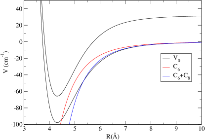
Figure 1: (Color online) Zero-field reference potentials. For the $V_{0}$ reference potential the first rotational excited state is also shown ($n=1$). The hard wall at $r=4.5$ Å is shown as a dashed line.

III.2 Comparison of full coupled-channel and MQDT results

III.2.1 Choice of $r_{\rm match}$ and reference potential

One of the goals of MQDT is to obtain a matrix $\bm{Y}(E,B)$ in such a way that it is only weakly dependent on energy $E$ and magnetic field $B$. However, the actual form of $\bm{Y}(E,B)$ is strongly dependent on the distance at which it is defined and the reference potentials used. In the present work we consider three different reference potentials, as shown in Figure 1. First we define a reference potential containing a pure $C_{6}$ long-range term, which has been used with great success in cold atom-atom collisions,

$$U^{\text{ref},C_{6}}_{i}(r)=-\frac{C_{6}}{r^{6}}+\frac{\hbar^{2}L_{i}(L_{i}+1)}{2\mu r^{2}}+E_{i}^{\infty},$$ (29)

where $C_{6}=7.621\times 10^{5}\text{ \AA}^{6}\text{ cm}^{-1}$ for Mg+NH Soldán et al. (2009). Secondly we define a reference potential containing an additional $C_{8}$ term,

$$U^{\text{ref},C_{6,8}}_{i}(r)=-\frac{C_{6}}{r^{6}}-\frac{C_{8}}{r^{8}}+\frac{\hbar^{2}L_{i}(L_{i}+1)}{2\mu r^{2}}+E_{i}^{\infty},$$ (30)

where $C_{8}=9.941\times 10^{6}\text{ \AA}^{8}\text{ cm}^{-1}$ Soldán et al. (2009). Finally we define

$$U^{\text{ref},V_{0}}_{i}(r)=V_{0}(r)+\frac{\hbar^{2}L_{i}(L_{i}+1)}{2\mu r^{2}}+E_{i}^{\infty},$$ (31)

where $V_{0}(r)$ is the isotropic part of the interaction potential, which is equivalent to the diagonal $\bm{W}$ matrix element in the incoming s-wave channel. Each reference potential contains a hard wall at $r=r^{\text{wall}}_{i}$, so that $U^{\text{ref}}_{i}(r)=\infty$ for $r<r^{\text{wall}}_{i}$. This allows the phase $\xi_{i}$ of the reference functions in each channel to be adjusted if required. A useful feature of MQDT, to be explored in future work, is that the position of the hard wall can be chosen to minimize the energy-dependence of $\bm{Y}$. However, in the present paper we simply take $r^{\text{wall}}_{i}=4.5$ Å.

It is convenient to compare MQDT and coupled-channel results at the level of T-matrix elements, $T_{ij}=\delta_{ij}-S_{ij}$. In general we label elements $T_{\alpha,L,M_{L}\rightarrow\alpha^{\prime},L^{\prime},M_{L}^{\prime}}$, where $|\alpha\rangle=|nsjm_{j}\rangle$. However, the collisions considered in the present paper are all among the $n=0,j=1$ levels and so $\alpha$ is simply abbreviated to $m_{j}$. The spin-changing cross sections are quite small except near resonances, so we focus mostly on diagonal elements, for which we suppress the second set of labels.

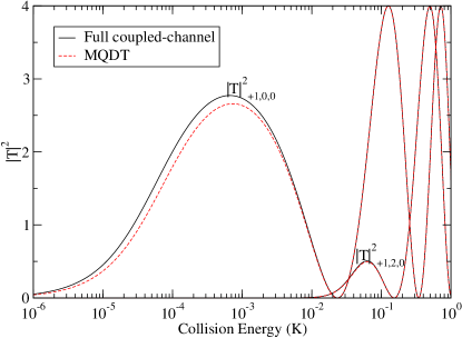
Figure 2: (Color online) The squares of diagonal $T$-matrix elements in the incoming channels for $m_{j}=+1$, $L=0$ and 2 at $B=10$ G, obtained from full coupled-channel calculations (solid, black) and MQDT with the $C_{6}$ reference potential and $r_{\text{match}}=20$ Å (dashed, red). $T$-matrix elements are labeled with quantum numbers $m_{j},L,M_{L}$. [Units of Gauss rather than Tesla, the accepted SI unit of magnetic field, have been used in this paper to conform to the conventional usage of this field.]

Figure 2 compares diagonal T-matrix elements $|T_{ii}|^{2}$ obtained from full coupled-channel calculations with those from the MQDT method for the pure $C_{6}$ reference potential of equation (29), with a matching distance of $r_{\text{match}}=20$ Å. The $\bm{Y}$ matrix was recalculated at every energy at which full coupled-channel calculations were performed. The MQDT results reproduce the coupled-channel results almost exactly at collision energies $E/k_{\rm B}>10$ mK. However, at lower energies the results start to differ noticeably. It may be noted that $|U_{i}^{\text{ref},C_{6}}-W_{ii}|/k_{\rm B}\approx 0.6$ mK at $r_{\text{match}}=20$ Å.

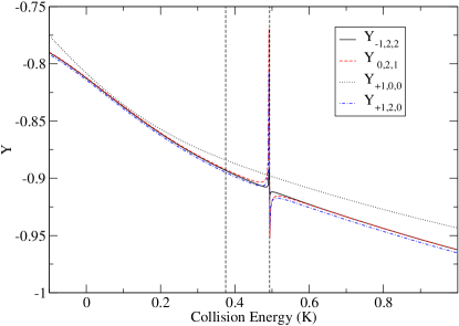
Figure 3: (Color online) Diagonal $\bm{Y}$ matrix elements as a function of collision energy at $B=10$ G for the $C_{6}$ reference potential with $r_{\text{match}}=20$ Å. The dashed vertical lines show the positions of quasibound states as described in the text.

Figure 3 shows the diagonal $\bm{Y}$ elements corresponding to Figure 2. They vary smoothly across most of the energy range, and are continuous across the threshold at zero energy, but exhibit occasional sharp structures as a function of energy. These sharp features are close to the energies of quasibound states, as shown by carrying out bound-state calculations using the BOUND package Hutson (1993), with the same basis set as the MOLSCAT calculations. The resulting bound-state energies are shown in Figure 3 as dashed vertical lines. The broad feature near $E/k_{\rm B}=0.5$ K is due to a quasibound state (Feshbach resonance) with quantum numbers $n=1$, $j=0$, $m_{j}=0$, $L=3$.

For MQDT to be more efficient than full coupled-channel calculations, it needs to produce results in agreement with full coupled-channel calculations from an energy-insensitive $\bm{Y}$ matrix that can be assumed to be constant or can be obtained by interpolation from a few energies, instead of being recalculated at every energy. However, the $\bm{Y}$ matrix elements in Figure 3 do not meet this requirement: the resonant features prevent reliable interpolation over useful ranges of energy.

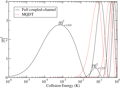
Figure 4: (Color online) The squares of diagonal $T$-matrix elements in the incoming channels for $m_{j}=+1$, $L=0$ and 2 at $B=10$ G, obtained from full coupled-channel calculations (solid, black) and MQDT with the $C_{6}$ reference potential and $r_{\text{match}}=6.8$ Å (dashed, red).

The energy sensitivity of the $\bm{Y}$ matrix in Figure 3 is due to the value used for $r_{\text{match}}$. When $r_{\text{match}}$ is large, resonance features due to quasibound states may be present in the log-derivative matrix from which $\bm{Y}$ is obtained. In this case the open and closed-channel blocks of $\bm{Y}$ are uncoupled, so that $\bar{\bm{Y}}\approx\bm{Y}_{\rm oo}$, and the resonances appear through the $\bm{Y}_{\rm oo}$ term in Eq. 21 rather than through $\tan\bm{\nu}+\bm{Y}_{\rm cc}$ Fourré and Raoult (1994). However, if $r_{\text{match}}$ is small enough, the resonance features are shifted to high energies, out of the region of interest. It is usually desirable to obtain $\bm{Y}$ at a value of $r_{\text{match}}$ that is in or near the classically allowed region for all weakly closed channels. However it must be remembered that the MQDT method neglects interchannel couplings that occur outside $r_{\text{match}}$, so there is always a tradeoff between choosing a value that minimizes the energy-dependence and one that takes account of coupling at relatively long range. This is particularly important in molecular scattering, where the anisotropy of the interaction potential often provides substantial couplings at long range.

It is convenient to consider lengths and energies in ultracold scattering in relation to the Van der Waals characteristic length and energy, defined by Jones et al. (2006)

$$r_{\text{VdW}}=\frac{1}{2}\left(\frac{2\mu C_{6}}{\hbar^{2}}\right)^{\frac{1}{4}}\text{\quad and \quad}E_{\rm VdW}=\frac{\hbar^{2}}{2\mu r_{\text{VdW}}^{2}}.$$ (32)

For Mg+NH, $r_{\text{VdW}}=12.7$ Å and $E_{\text{VdW}}/k_{\rm B}=11$ mK. In atomic systems, it is common to place $r_{\text{match}}$ close to $r_{\text{VdW}}$. However, the quasibound state responsible for the broad feature in Figure 3 is due to an $n=1$ state, with an outer turning point around 5.7 Å. The resonant feature therefore does not shift in energy significantly until $r_{\text{match}}$ is around 7 Å. In addition, it is not enough simply to move $r_{\text{match}}$ to short range with the same reference function. Figure 4 shows diagonal T-matrix elements obtained by MQDT with the $C_{6}$ reference function, as in Figure 2, but with $r_{\text{match}}=6.8$ Å. This does indeed produce a $\bm{Y}$ matrix without poles in the energy region of interest, but the MQDT results are no longer in agreement with the full coupled-channel results at any of the energies considered. This is because the difference between the reference potential and the diagonal $\bm{W}$ matrix elements at $r_{\text{match}}=6.8$ Å is $|U_{i}^{\text{ref},C_{6}}-W_{ii}|/k_{\rm B}\approx 4$ K, as seen in Figure 1. Alternatively, in terms of the approach of Mies and Raoult Mies and Raoult (2000), 6.8 Å is too short a distance for the $\bm{Y}$ matrix evaluated with the $C_{6}$ reference potential to have reached its asymptotic value.

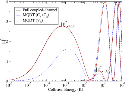
Figure 5: (Color online) The squares of diagonal $T$-matrix elements in the incoming channels for $m_{j}=+1$, $L=0$ and 2 at $B=10$ G, obtained from full coupled-channel calculations (solid, black) and MQDT with the $C_{6}+C_{8}$ (dot-dashed, blue) and $V_{0}$ (dashed, red) reference potentials and $r_{\text{match}}=6.8$ Å.

This problem may be remedied by using a better reference potential. Figure 5 shows results obtained using the reference potentials of equations (30) and (31), again for $r_{\text{match}}=6.8$ Å. The $C_{6}+C_{8}$ reference potential gives a marked improvement over the pure $C_{6}$ reference potential. The $\bm{T}$ matrix elements it produces follow the form of the full coupled-channel results but still become poor at energies much below 1 K: at $r_{\text{match}}=6.8$ Å, $|U_{i}^{\text{ref},C_{6}+C_{8}}-W_{ii}|/k_{\rm B}\approx 0.35$ K. However, the results obtained with the $V_{0}$ reference potential are much more accurate, and can scarcely be distinguished from the full coupled-channel results in Figure 5.

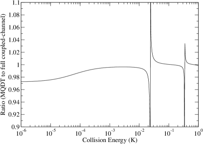
Figure 6: Ratio of the square of the diagonal $\bm{T}$ matrix element for $m_{j}=+1$, $L=0$ at $B=10$ G for MQDT, with the $V_{0}$ reference potential and $r_{\text{match}}=6.8$ Å, to that from full coupled-channel calculations.

Even the $V_{0}$ reference potential does not produce exact results. Figure 6 shows the ratio of the MQDT $T$-matrix elements for this reference potential to the full coupled-channel results. The poles in the ratio arise simply because MQDT places the zeroes in $|T|^{2}$ (where the phase shift is an integer multiple of $\pi$) at very slightly different collision energies. However, at very low energies (below about 1 mK) the MQDT results underestimate the squared $T$-matrix elements by up to 3%. This probably arises because the “best” reference potential would be one that takes account of adiabatic shifts due to mixing in excited rotational levels. For the $n=0$ channels, the shift due to $n=1$ channels may be estimated from 2nd-order perturbation theory to be about 0.012 cm^-1 (equivalent to 17 mK) at $r_{\text{match}}=6.8$ Å. This will cause residual errors in the MQDT $C$ functions that are responsible for the small errors visible in Figure 6.

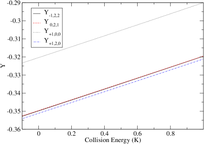
Figure 7: (Color online) Diagonal $\bm{Y}$ matrix elements as a function of energy at $B=10$ G, for the $V_{0}$ reference potential with $r_{\text{match}}=6.8$ Å.

Figure 7 shows representative matrix elements of $\bm{Y}$ obtained at $r_{\text{match}}=6.8$ Å, with the $V_{0}$ reference potential, as a function of energy. It may be seen that they are nearly linear in energy. The other matrix elements of $\bm{Y}$ show similar behavior. While the actual values of matrix elements vary substantially, they are all nearly linear in energy for $r_{\text{match}}=6.8\text{ \AA}$.

It should be noted that when the reference functions are obtained numerically, as in the present work, there is no significant difference in computer time for different choices of reference potential. Using the full $V_{0}$ reference potential is just as inexpensive as using a simpler one.

III.2.2 Feshbach resonances

Magnetic fields have important effects on cold molecular collisions, and in particular magnetically tunable low-energy Feshbach resonances provide mechanisms by which the collisions may be controlled. It is therefore important to establish whether the $\bm{Y}$ matrices obtained from MQDT are smooth functions of magnetic field as well as energy and can be used to characterize Feshbach resonances. If they are, it will offer substantial computational efficiencies.

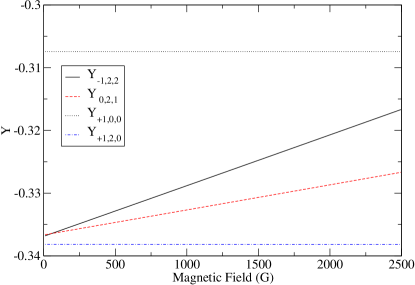
Figure 8: (Color online) Diagonal $\bm{Y}$ matrix elements as a function of magnetic field at $E/k_{\rm B}=400$ mK, for the $V_{0}$ reference potential with $r_{\text{match}}=6.8$ Å.

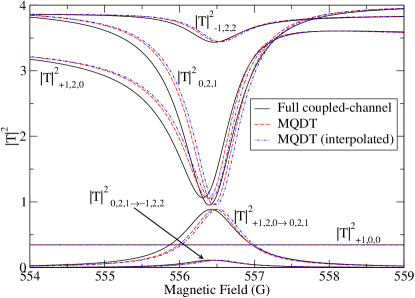
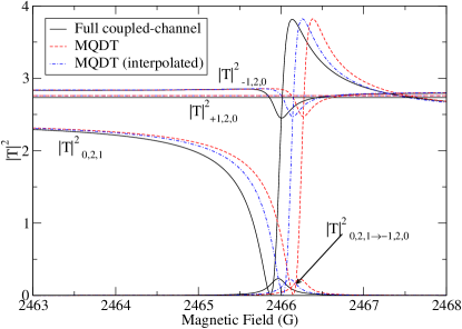
Figure 9: (Color online) Squares of diagonal and off-diagonal $T$-matrix elements as the field is tuned across a Feshbach resonance at $E/k_{\rm B}=400$ mK (upper panel) and 1 mK (lower panel). The MQDT results are obtained with the $V_{0}$ reference potential at $r_{\text{match}}=6.8$ Å.

Figure 8 shows how the diagonal $\bm{Y}$ matrix elements vary as a function of magnetic field for Mg+NH collisions over the range from 0 to 2500 G for a collision energy of 400 mK. It may be seen that the matrix elements are indeed very nearly linear, as required for efficient interpolation.

In Mg+NH, there is a Feshbach resonance due to the $n=1$, $j=0$, $m_{j}=0$, $L=3$ state shown in Figure 3 that tunes down towards the $n=0$, $m_{j}=+1$ threshold with increasing field. Figure 9 shows the comparison between MQDT and full coupled-channel calculations for a selection of diagonal and off-diagonal $\bm{T}$ matrix elements as the magnetic field is tuned across this resonance at energies of 400 mK and 1 mK. At each energy, MQDT results were obtained both by recalculating the $\bm{Y}$ matrix at every field and by linear interpolation between two points separated by 100 G. In both cases, the interpolated MQDT results are within about 0.2 G of the full MQDT results even for this long interpolation, and this could of course be improved simply by considering a few more fields across the range to allow. However, there is also a residual error of of 0.1 to 0.2 G in the resonance position even for the full MQDT results, which is not very different at the two collision energies considered. This is again likely to be due to the effect as described in Section III.2.1: the $V_{0}$ reference potential neglects couplings between channels outside $r_{\text{match}}$, and for the small value of $r_{\text{match}}$ used here these couplings are sufficient to shift the resonance positions slightly. Apart from these small shifts, however, both the elastic and the inelastic scattering around the resonances are very well described at both energies.

The linearity of the $\bm{Y}$ matrix with both energy and applied magnetic field is an extremely promising result, and suggests that MQDT will provide very efficient ways of performing cold collision calculations as a function of energy and magnetic field, without needing to repeat the expensive coupled-channel part of the calculation on a fine grid.

IV Conclusions

We have shown that Multichannel Quantum Defect Theory (MQDT) can be applied to low-energy molecular collisions in applied magnetic fields. MQDT provides a matrix $\bm{Y}$, defined at a distance $r_{\text{match}}$ at relatively short range, which encapsulates all the short-range dynamics of the system. For the prototype Mg+NH system, we have shown that MQDT can provide numerical results that are in quantitative agreement with full coupled-channel calculations if the MQDT reference functions are defined appropriately.

We have investigated the effect of different choices of reference potential and values of $r_{\text{match}}$. For cold atom-molecule collisions, unlike cold atom-atom collisions, calculations are likely to be needed over a significant range of collision energy, perhaps 1 K or so. If $r_{\text{match}}$ is placed at too long a range, there is a significant likelihood of resonant features within the energy range that prevent simple interpolation of $\bm{Y}$. This may be circumvented by carrying out the matching at a smaller distance $r_{\text{match}}$. However, when this is done, a pure $C_{6}$ reference potential may not be sufficient. For Mg+NH, the most satisfactory procedure is to perform matching at fairly short range (inside 7 Å) and use a reference potential that is defined to be the same as the true diagonal potential in the incoming channel.

The major strength of MQDT for molecular applications is that, if the the matching to obtain $\bm{Y}$ is carried out at relatively short range, the matrix is only weakly dependent on collision energy and magnetic field. This allows very considerable computational efficiencies, because the expensive calculation to obtain $\bm{Y}$ needs to be carried out at only one or a few combinations of collision energy and field. The remaining calculations to obtain scattering properties on a fine grid of energies and fields are then computationally inexpensive, varying only linearly with the number of channels $N$. Full coupled-channel calculations, by contrast, scale as $N^{3}$.

MQDT is a promising alternative to full coupled-channel calculations for cold atom-molecule collisions, particularly when fine scans over collision energy and magnetic field are required. In future work, we will investigate further the choice of reference functions to optimize the accuracy and to minimize the dependence of $\bm{Y}$ on collision energy and field. We will also investigate how the results for Mg+NH transfer to more strongly anisotropic systems, with stronger long-range anisotropy and more closed channels that are capable of producing scattering resonances.

V Acknowledgments

JMH is grateful to Chris Greene and John Bohn for interesting him in this project. The authors thank Maykel Leonardo González-Martínez and Jesus Aldegunde for exploratory work on molecular applications of MQDT at the beginning of the project. JFEC is grateful to EPSRC for a High-End Computing Studentship.

References

- Anderson et al. (1995) M. H. Anderson, J. R. Ensher, M. R. Matthews, C. E. Wieman, and E. A. Cornell, Science 269, 198 (1995).
- Davis et al. (1995) K. B. Davis, M.-O. Mewes, M. R. Andrews, N. J. van Druten, D. S. Durfee, D. M. Kurn, and W. Ketterle, Phys. Rev. Lett. 75, 3969 (1995).
- Doyle et al. (2004) J. Doyle, B. Friedrich, R. V. Krems, and F. Masnou-Seeuws, Eur. Phys. J. D 31, 149 (2004).
- Krems (2005) R. V. Krems, Int. Rev. Phys. Chem. 24, 99 (2005).
- Friedrich and Doyle (2009) B. Friedrich and J. M. Doyle, ChemPhysChem 10, 604 (2009).
- Hutson and Soldán (2006) J. M. Hutson and P. Soldán, Int. Rev. Phys. Chem. 25, 497 (2006).
- Ni et al. (2008) K.-K. Ni, S. Ospelkaus, M. H. G. de Miranda, A. Pe’er, B. Neyenhuis, J. J. Zirbel, S. Kotochigova, P. S. Julienne, D. S. Jin, and J. Ye, Science 322, 231 (2008).
- Ospelkaus et al. (2010) S. Ospelkaus, K.-K. Ni, D. Wang, M. H. G. de Miranda, B. Neyenhuis, G. Quéméner, P. S. Julienne, J. L. Bohn, D. S. Jin, and J. Ye, Science 327, 853 (2010).
- Danzl et al. (2010) J. G. Danzl, M. J. Mark, E. Haller, M. Gustavsson, R. Hart, J. Aldegunde, J. M. Hutson, and H.-C. Nägerl, Nature Phys. 6, 265 (2010).
- Hudson et al. (2002) J. J. Hudson, B. E. Sauer, M. R. Tarbutt, and E. A. Hinds, Phys. Rev. Lett. 89, 023003 (2002).
- Bethlem and Ubachs (2009) H. L. Bethlem and W. Ubachs, Faraday Discuss. 142, 25 (2009).
- DeMille (2002) D. DeMille, Phys. Rev. Lett. 88, 067901 (2002).
- Bell and P. Softley (2009) M. Bell and T. P. Softley, Mol. Phys. 107, 99 (2009).
- Weinstein et al. (1998) J. D. Weinstein, R. deCarvalho, T. Guillet, B. Friedrich, and J. M. Doyle, Nature 395, 148 (1998).
- Bethlem and Meijer (2003) H. L. Bethlem and G. Meijer, Int. Rev. Phys. Chem. 22, 73 (2003).
- Soldán and Hutson (2004) P. Soldán and J. M. Hutson, Phys. Rev. Lett. 92, 163202 (2004).
- deCarvalho et al. (1999) R. deCarvalho, J. Kim, J. D. Weinstein, J. M. Doyle, B. Friedrich, T. Guillet, and D. Patterson, Eur. Phys. J. D 7, 289 (1999).
- Lara et al. (2007) M. Lara, J. L. Bohn, D. E. Potter, P. Soldán, and J. M. Hutson, Phys. Rev. A 75, 012704 (2007).
- Żuchowski and Hutson (2009) P. S. Żuchowski and J. M. Hutson, Phys. Rev. A 79, 062708 (2009).
- Tokunaga et al. (2011) S. Tokunaga, W. Skomorowski, R. Moszynski, P. S. Żuchowski, J. M. Hutson, E. A. Hinds, and M. R. Tarbutt, Eur. Phys. J. D (2011), DOI: 10.1140/epjd/e2011-10719-x.
- Seaton (1966) M. J. Seaton, Proc. Phys. Soc. London 88, 801 (1966).
- Seaton (1983) M. J. Seaton, Rep. Prog. Phys. 46, 167 (1983).
- Greene et al. (1979) C. H. Greene, U. Fano, and G. Strinati, Phys. Rev. A 19, 1485 (1979).
- Greene et al. (1982) C. H. Greene, A. R. P. Rau, and U. Fano, Phys. Rev. A 26, 2441 (1982).
- Mies (1984) F. H. Mies, J. Chem. Phys. 80, 2514 (1984).
- Yoo and Greene (1986) B. Yoo and C. H. Greene, Phys. Rev. A 34, 1635 (1986).
- Gao (2008) B. Gao, Phys. Rev. A 78, 012702 (2008).
- Watanabe and Greene (1980) S. Watanabe and C. H. Greene, Phys. Rev. A 22, 158 (1980).
- Mies and Julienne (1984) F. H. Mies and P. S. Julienne, J. Chem. Phys. 80, 2526 (1984).
- Raoult and Balint-Kurti (1988) M. Raoult and G. G. Balint-Kurti, Phys. Rev. Lett. 61, 2538 (1988).
- Raoult and Balint-Kurti (1990) M. Raoult and G. G. Balint-Kurti, J. Chem. Phys. 93, 6508 (1990).
- Julienne and Mies (1989) P. S. Julienne and F. H. Mies, J. Opt. Soc. Am. B 6, 2257 (1989).
- Burke et al. (1998) J. P. Burke, C. H. Greene, and J. L. Bohn, Phys. Rev. Lett. 81, 3355 (1998).
- Mies and Raoult (2000) F. H. Mies and M. Raoult, Phys. Rev. A 62, 012708 (2000).
- Raoult and Mies (2004) M. Raoult and F. H. Mies, Phys. Rev. A 70, 012710 (2004).
- Gao et al. (2005) B. Gao, E. Tiesinga, C. J. Williams, and P. S. Julienne, Phys. Rev. A 72, 042719 (2005).
- Idziaszek et al. (2009) Z. Idziaszek, T. Calarco, P. S. Julienne, and A. Simoni, Phys. Rev. A 79, 010702 (2009).
- Gao (2010a) B. Gao, Phys. Rev. Lett. 104, 213201 (2010a).
- Idziaszek and Julienne (2010) Z. Idziaszek and P. S. Julienne, Phys. Rev. Lett. 104, 113202 (2010).
- Idziaszek et al. (2010) Z. Idziaszek, G. Quéméner, J. L. Bohn, and P. S. Julienne, Phys. Rev. A 82, 020703 (2010).
- Gao (2010b) B. Gao, Phys. Rev. Lett. 105, 263203 (2010b).
- Vogels et al. (2000) J. M. Vogels, R. S. Freeland, C. C. Tsai, B. J. Verhaar, and D. J. Heinzen, Phys. Rev. A 61, 043407 (2000).
- Gao (2001) B. Gao, Phys. Rev. A 64, 010701 (2001).
- Gao (1998a) B. Gao, Phys. Rev. A 58, 1728 (1998a).
- Gao (1998b) B. Gao, Phys. Rev. A 58, 4222 (1998b).
- Gao (2009) B. Gao, Phys. Rev. A 80, 012702 (2009).
- Julienne and Gao (2006) P. S. Julienne and B. Gao, AIP Conference Proceedings 869, 261 (2006).
- Gordon (1969) R. G. Gordon, J. Chem. Phys. 51, 14 (1969).
- Johnson (1973) B. R. Johnson, J. Comput. Phys. 13, 445 (1973).
- González-Martínez and Hutson (2007) M. L. González-Martínez and J. M. Hutson, Phys. Rev. A 75, 022702 (2007).
- Soldán et al. (2009) P. Soldán, P. S. Żuchowski, and J. M. Hutson, Faraday Discuss. 142, 191 (2009).
- Wallis and Hutson (2009) A. O. G. Wallis and J. M. Hutson, Phys. Rev. Lett. 103, 183201 (2009).
- Hutson and Green (2006) J. M. Hutson and S. Green, MOLSCAT computer program, version 14, distributed by Collaborative Computational Project No. 6 of the UK Engineering and Physical Sciences Research Council (2006).
- Alexander and Manolopoulos (1987) M. H. Alexander and D. E. Manolopoulos, J. Chem. Phys. 86, 2044 (1987).
- Numerov (1933) B. Numerov, Publs. Observatoire Central Astrophys. Russ. 2, 188 (1933).
- Johnson (1977) B. R. Johnson, J. Chem. Phys. 67, 4086 (1977).
- Hutson (1993) J. M. Hutson, BOUND computer program, version 5, distributed by Collaborative Computational Project No. 6 of the UK Engineering and Physical Sciences Research Council (1993).
- Fourré and Raoult (1994) I. Fourré and M. Raoult, J. Chem. Phys. 101, 8709 (1994).
- Jones et al. (2006) K. M. Jones, E. Tiesinga, P. D. Lett, and P. S. Julienne, Rev. Mod. Phys. 78, 483 (2006).