Generators of nonclassical states by combination of the linear coupling of boson modes, Kerr nonlinearity and the strong linear losses

Abstract

We show that the generators of quantum states of light can be built by employing the Kerr nonlinearity, a strong linear absorption or losses and the linear coupling of optical modes. Our setup can be realized, for instance, with the use of the optical fiber technology. We consider in detail the simplest cases of three and four coupled modes, where a strongly lossy mode is linearly coupled to other linear and nonlinear modes. In the three-mode design, our scheme emulates the third-order nonlinear absorption, allowing for generation of the single photon states, or the two-photon absorption allowing to generate the phase states. In the four-mode design, the scheme emulates a non-local absorption which produces an entangled state of two uncoupled modes. We also note that in the latter case and in the case of the phase states generation the output state is in the linear modes, which prevents its subsequent degradation by strong losses accompanying a strong Kerr nonlinearity.

I Introduction

Robust, efficient and reliable generators of nonclassical states of light are needed for the current and possible future technology. Nonclassical states are the working tools of quantum information and computation IC , besides other applications in quantum diagnostics and tomography, metrology, communications, etc. An ideal quantum state generator can be thought as a device producing a given quantum state by pushing a button, i.e. deterministically. It is known that a nonlinear media can be used to produce a nonclassical state of light from a classical (i.e. coherent) one TF , for instance, the $n$-photon Fock state can be obtained, at least in principle, in this way KCH . However, the experimental realization of the deterministic nonclassical state generators faces such great difficulties that the “determinism” requirement is currently dropped (it is pertinent to note that the overall efficiency of one of the most promising candidates for the “on-demand” single photons generation, the color centers in diamond, does not exceed a few percent CSD ). Instead, one has to be currently satisfied with the conditionally generated nonclassical states. For instance, the generation of the single photon states TF ; LO is currently based on producing the twin photon pairs by the parametric down-conversion or the heralded single photons generated in the mesoscopic $pn$ junctions pnT ; pnE .

The main difficulty of the deterministic nonclassical states generation using a nonlinear media is the losses, since a strong nonlinearity required for such a generator is inevitably accompanied by a strong absorption (in particular, this is the case of the nonlinear glasses used for fabrication of the nonlinear optical fibers). On the other hand, tailoring of a classical state to a nonclassical one by using the nonlinear absorption was also considered. Thus the dissipation, considered usually as a destructive effect to the fragile quantum features (e. g. the so-called “Schr$\mathrm{\ddot{o}}$dinger cat” quantum state is a proverbial example of this SCAT ), can be used also to drive the system into a nonclassical state (this is the essence of the “quantum state protection” DAV ). A wide variety of initial mixed states (or even an arbitrary mixed state) can be transformed into a desired pure state in this way, thus providing an extreme robustness of the scheme KRAUSS . The artificially designed dissipative systems were also shown to be the means of the quantum computation VWC .

The problem is that the practical realization of a given nonlinear loss channel for photons is rather difficult. One can engineer the dissipation needed for generating of the nonclassical states more or less freely working with the ions in a magnetic trap ZOLL ; WINL , or with the atoms in the optical lattices ZWER . However, designing similar reservoirs for photons is a much more challenging task, where even the theoretical schemes are mostly lacking. A notable exception is a couple of schemes proposed recently for generating of the phase states $(|0\rangle+e^{i\phi}|1\rangle)/\sqrt{2}$ TFAb ; TFComm ; TFRepl and the single-photon states NlAbs . Alas, they still require the very specific nonlinear dissipation (for example, the third-order nonlinear absorption is needed for the scheme of Ref. NlAbs ). Remarkably, in a recent work MS we have shown that one can emulate the needed nonlinear absorption by a simple design based on the optical coupler.

The purpose of the present work is to study in a more general setting the potential of our method of the quantum state generation, employed in Ref. MS . The central idea behind our scheme is the emulation of the needed nonlinear absorption by using a combination of the linear absorption, the Kerr-type nonlinearity and the mode coupling. It can be explained as follows. Consider a strongly lossy local mode linearly coupled to several other local modes. On the short evolution time (or propagation length), inversely proportional to the strong absorption, the lossy mode is emptied, whereas the rest of the modes are still significantly populated (curiously, this is due to the quantum Zeno effect Zeno ). Then the evolution can again be represented as that of a single lossy mode coupled to other modes but now in a coherent basis (i.e. a superposition of the local modes). Since some of the local modes are nonlinear – the usual Kerr nonlinearity is assumed – the coupling of this new lossy mode to other coherent modes is now nonlinear. When the coherent lossy mode is also emptied, the dynamics of the remaining coherent modes is governed by the nonlinear absorption, which can be tailored by selecting the particular setup of mode coupling. We show that, additionally to the single-photon states, also the phase states and the entangled states can be generated by our method. Moreover, output states in the second and third aforementioned examples are localized in the linear modes of the system, thus preventing the degradation of the output quantum state by the strong losses, always accompanying a strong Kerr nonlinearity.

The paper is organized as follows. In section II we describe the general scheme for the quantum state generation. We focus on the three coupled modes in section III, where we consider two nonlinear side modes, subsection III.1, and one nonlinear and one linear side modes, subsection III.2, coupled to a common lossy mode. Moreover, we study the generation of multi-photon Fock states by this scheme in subsection III.3. In section IV the case of four coupled modes is considered. In the Conclusion we outline the perspectives of the method.

II The general scheme for emulation of nonlinear losses

Our design for emulation of nonlinear absorption involves a boson mode subject to strong linear losses and coupled to other linear and nonlinear boson modes. We assume that the dynamics can be described by the master equation in the standard Lindblad form ME . For the system with Hamiltonian $H$ and a strongly lossy mode $b$, with the loss rate $\Gamma$, the evolution of an arbitrary operator $A(t)$ is given by the equation

$$\frac{dA}{dt}=i[H,A]+\Gamma\mathcal{D}[b^{\dagger}]A,$$ (1)

where $t$ is the evolution variable which will be called “time” for below (we use dimensionless variables), $\mathcal{D}[b^{\dagger}]A=b^{\dagger}Ab-\frac{1}{2}\{b^{\dagger}b,A\}$ (here and below the capital letters denote the time-dependent operators, while the small letters are used for the time-independent boson mode operators). We assume that the Hamiltonian $H$ can be expanded in the powers of the lossy mode as follows

$$H=\sum_{\alpha,\beta=0}{H}^{(\alpha,\beta)}(b^{\dagger})^{\alpha}b^{\beta}.$$ (2)

Here the coefficients ${H}^{(\alpha,\beta)}$ are operators in all other modes of the system. We limit our consideration to the Kerr nonlinearity, thus $\alpha,\beta\leq 2$ (note, however, that our method works for arbitrary nonlinearity).

Any time-dependent observable $A(t)$ can always be expanded in the infinite power series with respect to $b^{\dagger}$ and $b$:

$$A(t)=\sum_{\alpha,\beta\geq 0}A^{(\alpha,\beta)}(t)(b^{\dagger})^{\alpha}b^{\beta},$$ (3)

where the coefficients $A^{(\alpha,\beta)}(t)$ are time-dependent functions of the creation and annihilation operators of the other modes of the system.

For strong losses, i.e. $\Gamma\gg||H^{(\alpha,\beta)}||$, for the evolution times $t\gg 1/\Gamma$ the mode $b$ is almost empty and one can adiabatically eliminate it from the operator equation (1). The key observation is that the leading order term in the expansion, i. e. $A^{(0,0)}(t)$, is coupled by the Hamiltonian of Eq. (2) to just a few higher-order terms. The latter can be easily found in the explicit form in the adiabatic approximation. Inserting Eqs. (2) and (3) into Eq. (1) we have

$$\frac{dA^{(0,0)}}{dt}=i[H^{(0,0)},A^{(0,0)}]-iA^{(0,1)}H^{(1,0)}+iH^{(0,1)}A^{(1,0)}$$

$$+2iH^{(0,2)}A^{(2,0)}-2iA^{(0,2)}H^{(2,0)}.$$ (4)

Observing that for large times, $t\gg\Gamma$, the term $A^{(\alpha,\beta)}(t)$, with $\alpha+\beta>0$, decays as $\exp\{-\Gamma(\alpha+\beta)t/2\}$ we retain in the evolution equation for this term the only non-decaying term and the term multiplied by a large parameter (the decay rate $\Gamma$)

$$\frac{dA^{(\alpha,\beta)}}{dt}\approx i[H^{(\alpha,\beta)},A^{(0,0)}]-\frac{\Gamma(\alpha+\beta)}{2}A^{(\alpha,\beta)},$$ (5)

which results in

$$A^{(\alpha,\beta)}(t)\approx\frac{2}{\Gamma(\alpha+\beta)}[H^{(\alpha,\beta)},A^{(0,0)}(t)],\quad\alpha+\beta>0.$$ (6)

Finally, inserting the result (6) into Eq. (4), we arrive at the master equation with generally nonlinear artificial losses

$$\frac{dA^{(0,0)}}{dt}\approx i[H^{(0,0)},A^{(0,0)}]+\frac{4}{\Gamma}\sum_{\alpha=1,2}\mathcal{D}[H^{(0,\alpha)}]A^{(0,0)},$$ (7)

where the Lindblad generator $\mathcal{D}[\cdot]$ is defined below Eq. (1). Eq. (7) has the decay rate in the usual form of the quantum Zeno effect, i.e. the actual losses are inversely proportional to the bare loss rate $\Gamma$ Zeno .

Let us make the following observations about Eq. (7). Though we have assumed that the terms $H^{(0,1)}$ and $H^{(0,2)}$ in the expansion (2) of the Hamiltonian involve the nonlinearities, the strongly lossy mode is not required to be nonlinear (in fact, due to the strong loss, its nonlinearity is always negligible). Moreover, it is only linearly coupled to other modes of the system. Since Kerr nonlinearities are always diagonal in the spatially local boson basis, one needs the coupling to more than one mode, which makes such coupling diagonal in the non-local coherent basis and allows to emulate some nonlinear absorption. Thus, a linear coupling of a strongly lossy mode to two or more other modes, at least one of which is nonlinear, leads in the second adiabatic reduction to emulation of a nonlinear (coherent) lossy mode $b$ coupled to other nonlinear (coherent) modes.

We should mention the conditions which must be imposed for the adiabatic elimination of the lossy modes (in the two stages of the scheme) and the more important condition of the scheme efficiency related to the existence of the natural or induced (see below) linear losses. These conditions are particular to each realization of the general scheme and are given below for each example. We only mention that the first type of conditions are not actually necessary but only sufficient for the emulation of the nonlinear absorptions, but they allow an analytical treatment via the adiabatic elimination, as outlined above. The second type is more important, since, as we will see below, the linear losses, even not naturally present in the output modes, appear due to coupling to the lossy modes though with a significantly reduced rate (as in the case of the phase state generation, section III.2, and the generation of the entangled state, section IV). Moreover, both types of conditions point to the conclusion that a strongly asymmetric modal coupling is needed for the design of a specific nonlinear dissipation and the localization of the output nonclassical state in the local modes.

Finally, the system described by Eq. (7) can be realized using a fiber coupler or multi-core nonlinear fiber, where the optical mode of the central core is linearly coupled to the optical modes of the side cores/fibers, where some of the latter are made of the nonlinear media MS . In this case, the cores have to be the single-mode ones, however, the consideration can be generalized to the multi-mode case as well. Another possibility is to implement the electromagnetically induced transparency (EIT) media, where one can achieve a very high Kerr nonlinearity kerr (termed even the “giant Kerr nonlinearity”). Co-directional modes travelling through such a media can interact simultaneously and resonantly with the strongly damped emitters, in this way realizing the correlated loss of Eq. (2). A variation of this scheme is the propagation of several differently polarized modes in a nonlinear fiber with a strongly dissipative impurities (atoms, quantum dots, etc.) present in the core. When the average distance between impurities is much larger then the pulse length, the correlated modal loss can be achieved.

III Nonclassical state generation by the three mode coupler

Let us see how the above ideas can be applied for the case of three interacting modes. Recently, we have considered some particular realizations of this system MS ; SM . Here we analyze in detail the possibilities of the three-mode arrangement for generation of the nonclassical states, discussing the symmetrical and asymmetrical cases and the possibility of localization of the generated state in the mode with low losses. We consider the following Hamiltonian

$$H_{3}=\left[(g_{1}a_{1}+g_{2}a_{2})a^{\dagger}_{0}+h.c.\right]+\kappa_{1}(a_{1}^{\dagger})^{2}a_{1}^{2}+\kappa_{2}(a_{2}^{\dagger})^{2}a_{2}^{2},$$ (8)

where the strong loss is in mode $a_{0}$ with the loss rate $\Gamma_{0}$ such that $\Gamma_{0}\gg G=\sqrt{g_{1}^{2}+g_{2}^{2}}$ and $\Gamma_{0}\gg|\kappa_{1,2}|$ (here $g_{1,2}$ are real). The master equation for an observable $A=A(t,a^{\dagger}_{0},a_{0},a^{\dagger}_{1},a_{1},a^{\dagger}_{2},a_{2})$ of the whole system reads

$$\frac{dA}{dt}=i[H_{3},A]+\sum_{j=0}^{2}\Gamma_{j}\mathcal{D}[a^{\dagger}_{j}]A.$$ (9)

The first reduction of Eq. (9), given by Eq. (7) with the expansion in Eq. (3) in powers of $a^{\dagger}_{0}$ and $a_{0}$, features $H^{(0,1)}=\sum\limits_{j=1,2}g_{j}a^{\dagger}_{j}$ and $H^{(0,2)}=0$, and emulates the lossy coherent mode $b_{1}$ (with the linear losses rate $4G^{2}/\Gamma_{0}$) coupled to another coherent mode $b_{2}$. The new modes are given by the following rotation of local modes ($q=g_{1}/g_{2}$)

$$\left(\begin{array}[]{c}b_{1}\\ b_{2}\end{array}\right)=\left(\begin{array}[]{cc}\frac{q}{\sqrt{1+q^{2}}}&\frac{1}{\sqrt{1+q^{2}}}\\ -\frac{1}{\sqrt{1+q^{2}}}&\frac{q}{\sqrt{1+q^{2}}}\end{array}\right)\left(\begin{array}[]{c}a_{1}\\ a_{2}\end{array}\right).$$ (10)

Eq. (7) now involves the Lindblad terms for modes $b_{1,2}$ and the Hamiltonian describing the interaction of modes $b_{1}$ and $b_{2}$, which are derived from Eq. (9):

$$\sum_{j=1,2}\Gamma_{j}\mathcal{D}[a^{\dagger}_{j}]A=\sum_{j=1,2}\biggl{\{}\frac{q^{2}\Gamma_{j}+\Gamma_{j^{\prime}}}{1+q^{2}}\mathcal{D}[b^{\dagger}_{j}]A$$

$$+\frac{q(\Gamma_{2}-\Gamma_{1})}{1+q^{2}}\left(b^{\dagger}_{j}Ab_{j^{\prime}}-\frac{1}{2}\{b^{\dagger}_{j}b_{j^{\prime}},A\}\right)\biggr{\}},$$ (11)

$$H^{(0,0)}=\sum\limits_{j=1,2}\frac{\kappa_{j}}{1+q^{2}}(qb_{j}^{\dagger}+(-1)^{j}b_{j^{\prime}}^{\dagger})^{2}(qb_{j}+(-1)^{j}b_{j^{\prime}})^{2},$$ (12)

where $j^{\prime}=2$ for $j=1$ and vice versa.

We assume that the parameters are chosen in such way that mode $b_{1}$ has the shortest evolution time and can be adiabatically eliminated. We consider two particular limiting cases. In the first one both modes $a_{1,2}$ are carried by the nonlinear media with the same nonlinearity, thus $\kappa_{1}=\kappa_{2}$. In the second case only one of the two modes is nonlinear. As we shall see, there are significant differences between these cases.

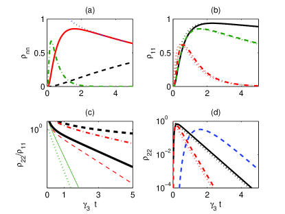
Figure 1: (Color online) (a) Dynamics of $\rho_{00}$ (dashed line), $\rho_{11}$ (solid line), $\rho_{22}$ (dash-dotted line) and average photon number (dotted line)as given by the solution of Eq. (13); $\Gamma=0.1\gamma_{3}$. (b) Dynamics of $\rho_{11}$ as given by Eq. (13) for the linear loss rate $\Gamma=0.01\gamma_{3}$, $0.1\gamma_{3}$, $\gamma_{3}$ (solid, dashed and dash-dotted lines). Dotted lines depict the solutions given by Eq. (19) for the corresponding values of $\Gamma$. (c) Dynamics of the ratio $\rho_{22}/\rho_{11}$ for $\Gamma=0.1\gamma_{3}$, $\gamma_{3}$, $10\gamma_{3}$ (thick solid, thin dashed, thin solid lines). Thick dashed, dash-dotted and dotted lines correspond to the same values of the linear rate, but with $\gamma_{3}$ being a hundred times smaller. (d) Dynamics of $\rho_{22}$ as given by Eq. (13) for the linear loss rate $\Gamma=0.1\gamma_{3}$ and $\Gamma=\gamma_{3}$ (solid and dashed). Dotted lines depict the solutions given by Eq. (19) for the corresponding values of $\Gamma$. In all figures $\gamma_{2}=0.01\gamma_{3}$, and the solution to Eq. (13) is found for the initial coherent state with the amplitude $z=7$.

III.1 Two nonlinear side modes: generation of the single-photon state

Let us consider first the case of two nonlinear side modes $a_{1,2}$, when one has $\kappa_{1}=\kappa_{2}\equiv\kappa$ and $\Gamma_{1}=\Gamma_{2}\equiv\Gamma$. This case was considered before MS as the scheme for the single-photon state generation. Here we turn our attention to the important problem of interplay between the linear and nonlinear losses arising on the long evolution time scale. Also, we outline some general features of dynamics produced by the artificial nonlinear losses.

In Ref. MS it was shown that after the modes $a_{0}$ and $b_{1}$ are emptied, the leading-order master equation for an observable $A=A(t,b^{\dagger}_{2},b_{2})$ becomes

$$\frac{dA}{dt}\approx i[H^{(0,0)},A]+\Gamma\mathcal{D}[b^{\dagger}_{2}]A+\gamma_{2}\mathcal{D}[(b^{\dagger}_{2})^{2}]A+\gamma_{3}\mathcal{D}[(b^{\dagger}_{2})^{2}b_{2}]A,$$ (13)

with the decay rates

$$\gamma_{2}=\frac{4\kappa^{2}q^{4}}{(1+q^{2})^{4}(\frac{4G^{2}}{\Gamma_{0}}+\Gamma)},\quad\gamma_{3}=\frac{4\kappa^{2}q^{2}(q^{2}-1)^{2}}{(1+q^{2})^{4}(\frac{4G^{2}}{\Gamma_{0}}+\Gamma)}$$ (14)

and the Hamiltonian

$$H^{(0,0)}=\frac{\kappa(q^{4}+1)}{2(1+q^{2})^{2}}n^{2}_{2}+\left(\frac{\kappa q^{2}}{(1+q^{2})^{2}}-\frac{\kappa}{2}\right)n_{2}.$$ (15)

We note that the symmetric coupling, i.e. $q=1$ leads to $\gamma_{3}=0$ (see Eq. (14)) and was considered recently in Ref. SM in the context of cold bosons in the triple-well trap. One of the notable results is that the two-photon dissipation (with the rate $\gamma_{2}$) cannot be captured by the mean-field approach, usually applied to systems of large number of bosons, though the induced linear dissipation is described by the mean-field model. Thus, quite naturally, one can expect of such a dissipation to generate nonclassical states.

When the linear and two-photon losses are absent ($\Gamma=0$ and $\gamma_{2}=0$), the scheme described by Eq. (13) is able to generate the single-photon state from a large amplitude coherent input NlAbs ; MS . Indeed, the purity of the output state can be easily estimated. The three-photon dissipation (with the rate $\gamma_{3}$) leaves the following operators invariant: $A_{00}=|0\rangle\langle 0|$, $A_{01}=|0\rangle\langle 1|$ and $A_{10}=A_{01}^{\dagger}$. Since for large times the density matrix $\rho$ involves only the Fock states $|0\rangle$ and $|1\rangle$, the following relations are valid:

$$\rho_{00}(\infty)=\rho_{00}(0),\;\rho_{10}(\infty)=\rho_{10}(0),\;\rho_{11}(\infty)=\sum_{k=1}^{\infty}\rho_{kk}(0).$$ (16)

Eq. (16) gives for the coherent input state $\rho(0)=|z\rangle\langle z|$ the following estimates: $\rho_{00}\approx e^{-|z|^{2}}$, $\rho_{10}\approx ze^{-|z|^{2}}$ and $\rho_{11}\approx 1-e^{-|z|^{2}}$. Thus, for $|z|\gg 1$ and $t\gg 1/\gamma_{3}$ the density matrix $\rho$ is exponentially close to the single photon state $|1\rangle\langle 1|$, i.e. $1-\mathrm{Tr}\{\rho^{2}\}\approx 2e^{-|z|^{2}}$.

Since neither of $g_{j}$ can be zero, the two-photon losses are also inevitable. However, for a strong asymmetry, e.g. $|g_{1}|\gg|g_{2}|$, we get $\gamma_{3}/\gamma_{2}=(q-1/q)^{2}\gg 1$. Therefore the three-photon decay channel dominates, resulting in the single-photon state generation from any coherent input with a large amplitude MS . For example, for $|q|=10$ the fidelity of the single-photon state generation can exceed $99\%$. For such an asymmetric coupling, in the absence of the linear losses, the resulting state is approximated by the following one

$$|\textrm{out}\rangle\approx\frac{1}{\sqrt{1+q^{2}}}\left[q|0\rangle_{1}|1\rangle_{2}-|1\rangle_{1}|0\rangle_{2}\right],$$ (17)

i.e. the photon is carried mostly by the weakly coupled mode $a_{2}$. The linear losses, however, gradually degrade the generated state. For example, for the linear loss rate an order of magnitude smaller than $\gamma_{3}$, the fidelity of the single-photon state generation drops to $86\%$ MS . The effect of the linear loss is smaller for smaller times. However, in that case a significant multi-photon contribution to the state is still present (Fig. 1(a)). The multi-photon component can be a significant obstacle for using the generated state in the quantum cryptography protocols, where a presence of the two-photon component in the signal can be used for security breaking LO .

For small linear losses one can obtain a simple estimate of the parameters range when there is a significant probability of the single-photon state simultaneously with a small probability of the multi-photon components in the signal. We note that in the Fock state basis only the elements $\rho_{n,n+k}$ with a fixed $k$ of the density matrix are coupled by Eq. (13). The diagonal elements satisfy the following equation

$$\frac{d\rho_{nn}}{dt}=\sigma_{n}\rho_{n+2,n+2}+\beta_{n}\rho_{n+1,n+1}-\Gamma_{n}\rho_{nn},$$ (18)

where $\sigma_{n}=(n+2)(n+1)\gamma_{2},\quad\beta_{n}=(n+1)(\Gamma+n^{2}\gamma_{3})$ and $\Gamma_{n}=n[\Gamma+(n-1)\gamma_{2}+(n-1)^{2}\gamma_{3}]$. Assuming that the mode $b_{2}$ is initially in the two-photon Fock state, from Eq. (18) one easily obtains

$$\rho_{22}=\exp{\left\{-2(\Gamma+\gamma_{2}+\gamma_{3})t\right\}},$$

$$\rho_{11}=\frac{\gamma_{3}+\Gamma}{\gamma_{2}+\gamma_{3}+\Gamma/2}$$

$$\times\left(\exp\left\{-\Gamma t\right\}-\exp\left\{-2(\Gamma+\gamma_{2}+\gamma_{3})t\right\}\right)$$ (19)

and $\rho_{00}=1-\rho_{11}-\rho_{22}$.

It is interesting that the simple estimate (19) gives a fairly accurate approximation of the single-photon generation fidelity (i.e. $\rho_{11}$) for times when the initially coherent state of mode $b_{2}$ approaches the single-photon level (Fig. 1(b)). The approximation is quite precise even for the linear decay rate approaching $\gamma_{3}$. One can see that the position of the fidelity maximum is also captured quite precisely. Apart from the initial time interval when the state is far from the single-photon state, the estimate (19) describes quite accurately the behavior of the two-photon component, $\rho_{22}$ (Fig. 1(d)).

Eq. (19) allows to estimate $\rho_{22}/\rho_{11}$ at the time when the output state attains its maximal fidelity of the single-photon component. This latter time, $T$, is defined by the condition $d\rho_{11}/dt=0$ and reads

$$T=\frac{1}{2\gamma_{2}+2\gamma_{3}+\Gamma}\ln\left(1+\frac{\gamma_{2}+\gamma_{3}}{\Gamma}\right).$$ (20)

This estimate of the fidelity maximum gives a very simple result for the ratio

$$\frac{\rho_{22}(T)}{\rho_{11}(T)}=\frac{\Gamma}{\Gamma+\gamma_{3}}.$$ (21)

This result seems rather disappointing, since for having a small ratio $\rho_{22}/\rho_{11}$ at the maximal single-photon fidelity one needs to have the linear loss rate much smaller then the nonlinear one, $\Gamma\ll\gamma_{3}$. However, if we relax the condition of having the maximal possible single-photon fidelity, then even a strong linear loss does not eliminate the applicability of our scheme for the single-photon state generation. Eq. (19) shows that $\rho_{22}$ decays faster than in the linear case, and $\rho_{11}$ decays much slower. Even for the linear loss rates exceeding $\gamma_{3}$, our scheme is an advantage if compared to the simple linear attenuating of a coherent state (Fig. 1(c)).

III.2 The nonclassical states generation with one nonlinear and one linear side modes

Now let us consider the asymmetrical case, when only one of the side modes is carried by nonlinear (and, consequently, lossy) media. We assume that $\kappa_{2}=0$, $\kappa_{1}\equiv\kappa$, and the rate of the linear loss is much less than that of the nonlinear one, $\Gamma_{2}\ll\Gamma_{1}$. The nonlinear term of the Hamiltonian (8), written in the $b$-basis, defines the nonlinear decay channels. Expanding in terms of $b^{\dagger}_{1}$ and $b_{1}$ we get the operator coefficients (see Eq. (2)):

$$H^{(0,1)}=-\frac{2q\kappa}{(1+q^{2})^{2}}(b^{\dagger}_{2})^{2}b_{2},\quad H^{(0,2)}=\frac{q^{2}\kappa}{(1+q^{2})^{2}}(b^{\dagger}_{2})^{2}.$$ (22)

The coupling asymmetry defines the resulting quantum state and the output channel (in this case, the local mode $a_{1}$ or $a_{2}$).

The single-photon state generation.– First, we consider the case of $q\ll 1$, which leads to the localization of the coherent modes as follows $b_{1}\approx a_{2}+qa_{1}$ and $b_{2}\approx-a_{1}+qa_{2}$. Note that, since mode $b_{1}$ is empty, the r.h.s. of Eq. (11) simplifies in this case to the diagonal form with the loss rate $\Gamma_{b_{2}}\approx\Gamma_{1}+q^{2}\Gamma_{2}$ (note that the contribution from the linear losses are negligible since $q^{2}\Gamma_{2}\ll\Gamma_{1}$). Resuming, when the modes $a_{0}$ and $b_{1}$ are emptied, the leading-order master equation for an observable $A=A(t,b^{\dagger}_{2},b_{2})$ becomes

$$\frac{dA}{dt}\approx i[H^{(0,0)}\!\!,A]+\Gamma_{b_{2}}\mathcal{D}[b^{\dagger}_{2}]A+\gamma_{2}\mathcal{D}[(b^{\dagger}_{2})^{2}]A+\gamma_{3}\mathcal{D}[(b^{\dagger}_{2})^{2}b_{2}]A,$$ (23)

with $H^{(0,0)}=\kappa(b^{\dagger}_{2})^{2}b_{2}^{2}$ and the loss rates

$$\gamma_{2}\approx\frac{16q^{4}\kappa^{2}}{4G^{2}/\Gamma_{0}+\Gamma_{1}},\quad\gamma_{3}\approx\frac{16q^{2}\kappa^{2}}{4G^{2}/\Gamma_{0}+\Gamma_{1}},$$

i.e. $\gamma_{2}/\gamma_{3}\approx q^{2}\ll 1$, which is the condition for the single-photon state generation NlAbs . This scheme is similar to our previous proposal MS , considered in section III.1, but involves just one nonlinear side mode. The single-photon state is still localized in the nonlinear mode ($a_{1}$). Below we also present the schemes which generate quantum states in the linear output modes of the system (whether such a scheme exists for the single-photon generation is yet unknown).

The evolution interval for the generation of single-photons is quite similar as in Fig. 1 and given by the condition $1/\gamma_{3}\ll t\ll 1/\Gamma_{1}$. The sufficient conditions (used in the two reductions and the efficiency condition) for the single-photon generation read:

$$\frac{G}{\Gamma_{0}}\ll 1;\;\kappa,\,q\Gamma_{1}\ll\frac{G^{2}}{\Gamma_{0}};\;\frac{G^{2}\Gamma_{1}}{\Gamma_{0}}\ll(q\kappa)^{2},$$ (24)

where the last condition is needed for efficiency of the generator. The consistency of conditions (24) requires that ${\Gamma_{1}\Gamma_{0}}/{G^{2}}\ll q^{2}$, i.e. the efficiency of the generator is limited by the losses in the nonlinear Kerr mode.

The phase state generation.– Let us now consider the case of $q\gg 1$, which also leads to the nonclassical states generation. In this case the scheme emulates the two-photon absorption, as is seen from Eq. (22). Therefore, for an initial coherent state, $|z\rangle$ with $|z|\sim 1$, the output density matrix of mode $b_{2}$ is very close to the phase state $|0\rangle+e^{i\arg(z)}|1\rangle$ TFAb ; TFComm ; TFRepl . Note that the output mode is still given by $b_{2}$, however now it is localized in the linear mode, $b_{2}\approx a_{2}-q^{-1}a_{1}$. We have the same form of the approximate master equation (23) but now with the reduced Hamiltonian $H^{(0,0)}\approx(\kappa/q^{4})(b^{\dagger}_{2})^{2}b^{2}_{2}$, $\gamma_{3}\approx\frac{4\kappa^{2}\Gamma_{0}}{q^{6}G^{2}}$ and $\gamma_{2}\approx\frac{\kappa^{2}\Gamma_{0}}{q^{4}G^{2}}$, with $\gamma_{3}/\gamma_{2}\approx q^{-2}\ll 1$, where we have assumed that the linear mode $a_{2}$ has negligible losses. Moreover, since the operating mode $b_{2}$ is almost localized in the linear mode $a_{2}$ the linear loss rate of this mode is almost equal to that of mode $a_{2}$, i.e. we have from Eq. (11) in this case: $\Gamma_{b_{2}}\approx\Gamma_{2}+\Gamma_{1}/q^{2}$ (the cross-term vanishes since the mode $b_{1}$ is empty). The necessary conditions on the scheme parameters in this case read

$$\frac{G}{\Gamma_{0}}\ll 1,\;qG\sqrt{\frac{\Gamma_{1}}{\Gamma_{0}}}\ll\kappa\ll\frac{G^{2}}{\Gamma_{0}},$$ (25)

with a similar consistency condition as for the single-photon generator, i.e. ${\Gamma_{1}\Gamma_{0}}/{G^{2}}\ll 1/q^{2}$.

III.3 Generation of the multi-photon nonclassical states

Usefulness of the three-mode scheme for generating of the nonclassical states is not limited to generation of the single-photon and phase states. As it was mentioned in the Introduction, the nonlinear decay can be designed to produce an arbitrary quantum state. In particular, the nonlinear dissipation with the Lindblad generator of the type as in Eq. (13), i.e. $f(n_{2})b^{\dagger}_{2}$, where $f(x)$ is a positive definite function, in the absence of the linear losses can lead to the stationary superposition of any given number of Fock states, or even to the “combing” of the initial coherent state by retaining only the components with either even or odd photon numbers mich .

Moreover, for a sufficiently small evolution time even Eq. (13) can lead to strongly nonclassical states. In generation of such states our scheme can be much more robust with respect to the linear losses than in generation of the single-photon state. It is easy to see that the modal dynamics in the presence of nonlinear loss can be fairly impervious to the linear decay for times much smaller than the characteristic time of both linear and nonlinear decay. This can be shown by invoking an argument from the quantum jumps theory. Let us assume, for simplicity, that the evolution is purely dissipative (the Hamiltonian is zero). Then the quantum Monte-Carlo trajectory, $|\psi(t)\rangle$, undergoes random jumps described by the Lindblad operator $L$ ME :

$$|\psi(t)\rangle\rightarrow L|\psi(t)\rangle.$$

The probability of the jump is proportional $\langle\psi(t)|L^{\dagger}L|\psi(t)\rangle$. Obviously, the state components with the high photon numbers will be “jumping down” via the nonlinear decay described by Eq. (13) with much larger rate than that of the linear decay. For instance, it was shown that for $L=b_{2}^{2}$ quite different initial states decay to the stationary state practically in the same time DodMiz .

Thus, one can expect that a classical state can be transformed into a nonclassical one by the scheme described by Eq. (13) in a short evolution time for which the linear losses are still negligible. Indeed, for two nonlinear side modes, when $\gamma_{3}\gg\gamma_{2}$, one should expect a significant change of the quantum state to occur for the evolution time on the order

$$t\sim\left(\gamma_{3}\langle n_{2}^{2}\rangle\right)^{-1}.$$ (26)

Fig. 2(a) confirms this prediction (there the expected significant change occurs at $\gamma_{3}t\approx 0.0004$, i.e. exactly at the estimate (26)). For such times the average number of photons drops by nearly two times. Naturally, the linear decay rate should be of several orders of magnitude larger than the nonlinear one to play any significant role in this case.

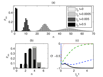
Figure 2: (Color online) (a) Evolution of the photon-number distribution for small losses $\Gamma=0.1\gamma_{3}$. (b) The photon-number distribution at $\gamma_{3}t=0.3$; light gray, dark gray and black bars correspond to $\Gamma=0$,$0.1\gamma_{3}$ and $\gamma_{3}$. (c) The corresponding Mandel parameter $Q$, given by Eq. (27), for $\Gamma=0$, $0.1\gamma_{3}$, $\gamma_{3}$ and $10\Gamma_{3}$ (solid, dashed, dash-dotted and dotted curves). We use the solution of Eq. (13) for the initial coherent state with the amplitude $z=7$. Here $\gamma_{2}=0.01\gamma_{3}$.

We also note that even for larger times and a smaller average photon number the generated state is quite robust with respect to the linear losses. For example, for the states with three or four photons on average, the linear losses with the rate even comparable with $\gamma_{3}$ do not destroy the nonclassicality (Fig. 2(b,c)). It is interesting that for moderate linear losses the few-photon states, generated this way, can be very interesting. One can obtain, for instance, a nearly equal mixture of the one and two-photon components, Fig. 2(a).

The nonclassicality of the generated state can be illustrated by using the Mandel parameter,

$$Q=\frac{\langle n_{2}^{2}\rangle-\langle n_{2}\rangle^{2}}{\langle n_{2}\rangle}-1,$$ (27)

which is zero for a coherent state. It is seen from Fig. 2(c) that for the initial coherent state the generated state is manifestly a sub-Poissonian one during all $t>0$. In the absence of linear losses one can distinguish three stages of the $Q$-parameter evolution. First, it sharply drops (for the time-scale given by the estimate (26)). Then, when the state has a sharp few-photon maximum, the Mandel parameter oscillates. Finally, it slowly approaches $Q_{F}=-1$, i.e. its value for a Fock state.

For the small and moderate linear loss rate, $\Gamma\leq\gamma_{3}$, only the third stage appears to be affected: the Mandel parameter rises slowly towards zero. As long as the linear decay rate remains larger then the time-scale given by the estimate (26), the first stage is practically unaffected. During this stage, the quantum state undergoes strong photon-number squeezing.

Thus the considered scheme can serve as an efficient and robust practical source of the sub-Poissonian nonclassical states. Obviously, all kinds of set-ups mentioned above serve for this purpose. For example, a few centimeters of the three-core fiber with the realistic nonlinearity and linear losses is enough for reaching $Q\sim 0.1$ MS .

We conclude that the multi-core fiber realizations of the scheme described in section II can be quite useful for generating of the multi-photon nonclassical states despite the fact that a strong Kerr nonlinearity is usually accompanied by a strong linear absorption. Linear losses can be dealt with more efficiently in the scheme with the individual damped emitters (quantum dots, atoms, color defects etc.) acting as a common loss reservoir for the light modes. Moreover, the EIT-like schemes exhibiting a very strong Kerr-nonlinearity kerr might be a promising candidate for realization of our setup.

IV The entangled state generation by the four-mode coupler

Let us now explore a four-mode generalization of our scheme. We assume that a strongly lossy mode $a_{0}$ is coupled to three other modes, one from which is a nonlinear mode, $a_{3}$, and two other are linear ones, $a_{1,2}$. We consider the Hamiltonian

$$H_{4}=G\left(a^{\dagger}_{0}\sum_{\ell=1}^{3}g_{\ell}a_{\ell}+a_{0}\sum_{\ell=1}^{3}g_{\ell}a^{\dagger}_{\ell}\right)+\kappa(a^{\dagger}_{3})^{2}a_{3}^{2},$$ (28)

where the coupling coefficients $g_{\ell}$ are real and normalized $\sum_{\ell}g^{2}_{\ell}=1$. Moreover, for specific localization of the coherent modes (see below) the $g_{\ell}$ are assumed to be strongly asymmetric: $g_{1}=g_{2}=\epsilon\ll 1$ and $g_{3}=1-\mathcal{O}(\epsilon^{2})$. The master equation for the observable $A$ of the system reads

$$\frac{dA}{dt}=i[H_{4},A]+\Gamma_{0}\mathcal{D}[a^{\dagger}_{0}]A+\Gamma_{3}\mathcal{D}[a^{\dagger}_{3}]A,$$ (29)

where we neglect the losses in the linear modes $a_{1,2}$ and assume that the strong dissipation of mode $a_{0}$ has the shortest time scale, i.e. $\Gamma_{0}\gg G,\Gamma_{3},\kappa$. To perform the steps which lead us to the second reduction, Eq. (7), we need to introduce a coherent basis $b_{\ell}$ given by the unitary matrix $U$ with the constraint $U_{\ell,3}=(g_{1},g_{2},g_{3})$. This matrix can be chosen as follows

$$\left(\begin{array}[]{c}b_{1}\\ b_{2}\\ b_{3}\end{array}\right)=\left(\begin{array}[]{ccc}\sqrt{1-g_{1}^{2}}&-\frac{g_{1}g_{2}}{\sqrt{1-g^{2}_{1}}}&-\frac{g_{1}g_{3}}{\sqrt{1-g^{2}_{1}}}\\ 0&\frac{g_{3}}{\sqrt{1-g^{2}_{1}}}&-\frac{g_{2}}{\sqrt{1-g^{2}_{1}}}\\ g_{1}&g_{2}&g_{3}\end{array}\right)\left(\begin{array}[]{c}a_{1}\\ a_{2}\\ a_{3}\end{array}\right).$$ (30)

In the strongly asymmetric case, the rotation (30) can be approximated as $b_{\ell}=a_{\ell}-\epsilon a_{3}+\mathcal{O}(\epsilon^{2})$, $\ell=1,2$ and $b_{3}=a_{3}+\epsilon(a_{1}+a_{2})+\mathcal{O}(\epsilon^{2})$. In this case, the adiabatic procedure described in Section II eliminates the lossy mode $a_{0}$ (the first stage) and then the coherent mode $b_{3}$ (the second stage). For the evolution times $t\gg 1/(\Gamma_{3}+4G^{2}/\Gamma_{0})$, i.e. when mode $b_{3}$ is already in the vacuum state, the two coherent modes $b_{1,2}$ possess two channels of decay, as given by Eq. (7). These channels correspond to the two Lindblad generators $H^{(0,1)}$ and $H^{(0,2)}$ obtained by the expansion (as in Eq. (2)) of Hamiltonian (28) in powers of $b^{\dagger}_{3}$ and $b_{3}$. In the leading order approximation we have:

$$H^{(0,1)}=-\epsilon^{3}\kappa(b^{\dagger}_{1}+b^{\dagger}_{2})^{2}(b_{1}+b_{2})+\mathcal{O}(\epsilon^{5}),$$

$$H^{(0,2)}=\epsilon^{2}\kappa\left[(b^{\dagger}_{1})^{2}+(b^{\dagger}_{2})^{2}+b^{\dagger}_{1}b^{\dagger}_{2}\right]+\mathcal{O}(\epsilon^{4}),$$ (31)

hence the corresponding decay rates in Eq. (7) (with $\Gamma=\Gamma_{3}+4G^{2}/\Gamma_{0}$) read $\gamma_{2}\approx 4\epsilon^{4}\kappa^{2}/(\Gamma_{3}+4G^{2}/\Gamma_{0})$ and $\gamma_{3}\approx 4\epsilon^{6}\kappa^{2}/(\Gamma_{3}+4G^{2}/\Gamma_{0})$. The reduced two-mode Hamiltonian is $H^{(0,0)}=\epsilon^{4}\kappa(b^{\dagger}_{1}+b^{\dagger}_{2})^{2}(b_{1}+b_{2})^{2}$.

The output states of this four-mode scheme are localized in the linear modes $a_{1,2}$. Note that the coupling to the lossy nonlinear mode $a_{3}$ induces the coherent linear losses with the Lindblad generator $b_{1}^{\dagger}+b_{2}^{\dagger}$ and a reduced loss rate $\Gamma_{L}\equiv\epsilon^{2}\Gamma_{3}$, which fact can be easily established by expansion of the term $\Gamma_{3}\mathcal{D}[a_{3}^{\dagger}]=\Gamma_{3}\mathcal{D}[\sum_{k}U_{k3}b_{3}^{\dagger}]$ similar as in Eq. (11). For below, we can neglect the decay channel $H^{(0,1)}$, with the decay rate $\gamma_{3}$, as compared to the channel $H^{(0,2)}$ and the linear losses.

The sufficient conditions for the adiabatic elimination of the lossy modes and the condition of the scheme efficiency read

$$\Gamma_{0}\gg G,\Gamma_{3},\kappa;\quad\epsilon^{2}\kappa\ll\Gamma_{3}+\frac{4G^{2}}{\Gamma_{0}}\ll\epsilon\kappa,$$ (32)

with the simple unrestrictive consistency condition $\epsilon\ll 1$ (cf. with that for the three-mode scheme of section III). In Eq. (32) the rightmost inequality is the requirement of the scheme efficiency (the artificial nonlinear loss rate $\gamma_{2}$ is stronger than the induced linear loss in $a_{1,2}$), while the middle one together with the left one (already mentioned above) are sufficient conditions for the adiabatic elimination of the lossy modes. Under these conditions, the strongest nonlinear dissipation, with $H^{(0,2)}$, the linear losses term $\Gamma_{L}\mathcal{D}[b_{1}^{\dagger}+b_{2}^{\dagger}]$ and the reduced Hamiltonian $H^{(0,0)}$ together govern the evolution of observables.

If the liner losses were absent, the nonlinear losses term would dominate the Hamiltonian part, since $\gamma_{2}\gg\epsilon^{4}\kappa$, i.e. $\kappa\gg\Gamma_{3}+4G^{2}/\Gamma_{0}$, which is satisfied due to conditions (32). To find out what structure the output density matrix has, let us simplify the Lindblad generators by performing a rotation to the coherent basis:

$$c_{\pm}=\frac{b_{1}\pm b_{2}}{\sqrt{2}}=\frac{a_{1}\pm a_{2}}{\sqrt{2}}-\epsilon\sqrt{2}a_{3}+\mathcal{O}(\epsilon^{2}).$$ (33)

We have $H^{(2,0)}=\epsilon^{2}\kappa(3c_{+}^{2}-c_{-}^{2})/2$ and $H^{(0,0)}=4\epsilon^{4}\kappa(c^{\dagger}_{+})^{2}c^{2}_{+}$. Then, up to the order $\epsilon^{4}$ the master equation (now written for the density matrix, in the coherent basis) reads

$$\frac{d\rho}{dt}=-i[H^{(0,0)},\rho]+\gamma_{2}\mathcal{D}[(3c_{+}^{2}-c_{-}^{2})/2]\rho+2\Gamma_{L}\mathcal{D}[c_{+}]\rho.$$ (34)

The nonlinear loss term has the null subspace given by the following expansion in the Fock basis of the coherent modes

$$|\textrm{null}\rangle=\sum_{n,m}f(n)g(m)|n,m\rangle,$$ (35)

where each $n$ and $m$ take only even or odd values (independently), while $f(k)=\frac{f_{0}}{3^{k/2}\sqrt{k!}}$ and $g(l)=\frac{g_{0}}{\sqrt{l!}}$. Note that the coherent state $|\alpha,\sqrt{3}\alpha\rangle$ belongs to this null subspace. However, only the following Fock basis vectors

$$|0,0\rangle,\;|0,1\rangle,\;|1,0\rangle,\;|1,1\rangle,$$ (36)

belong to the joint null subspace of $H^{(2,0)}$ and $H^{(0,0)}$.

We will further concentrate on the realistic case with the conditions (32) satisfied, i.e. when there is also the linear loss term and the decay rates are ordered as follows

$$\gamma_{3}\ll\epsilon^{4}\kappa\ll\Gamma_{L}\ll\gamma_{2}.$$

In this case the output density matrix can be found only numerically. Since the initial dynamics (i.e. effecting the two adiabatic reductions) almost leaves the non-dissipated modes unaffected, the state of these modes is close to the initial state. Hence, one can pass to simulating the resulting approximate master equation (34) instead of that for the four coupled modes. While the average values can be found numerically without much effort for quite large amplitudes of the initial coherent state, the entanglement measure (see below) requires knowledge of the whole underlying density matrix. This limits the efficiency of the numerical simulations and we are able to simulate thoroughly only the small amplitude case of $|\alpha_{j}|\sim 1$.

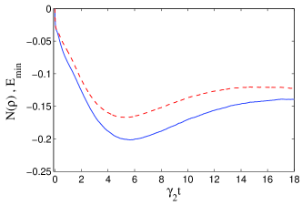
Figure 3: (Color online) The entanglement witness (solid), the sum of the negative eigenvalues of the partial transpose of the density matrix of modes $a_{1,2}$ restricted to Fock indices $n\in\{0,...,5\}$ in each mode, and the corresponding lowest negative eigenvalue (dashed). Here the parameters read $\epsilon=0.1$, $\kappa=30$, $\Gamma_{0}=10$ and $\Gamma_{3}=2$ which give $\gamma_{2}=0.15$, $\epsilon^{4}\kappa=0.012$ and $\Gamma_{L}=0.024$. We have used the following coherent state $|-i\alpha,0.9\alpha\rangle$ as the input state with $\alpha=1.6$ (using another input state with the similar average number of photons does not change the picture). The figure is an average over 17000 quantum trajectories.

Fortunately, considering the small amplitude case is sufficient for concluding on the general case. This is because the nonlinear Lindblad term of the master equation (34) admits some integral invariants, which are also invariants of the Hamiltonian dynamics. Indeed, since in the absence of the linear losses the photons are removed by pairs, the Hilbert space of each of the coherent modes is effectively divided into two subspaces, involving only either even or odd Fock number states. Hence, introducing the identity operators in each parity subspace, $I_{ev}$ and $I_{odd}$, the above mentioned integral invariants are given by taking the trace of four possible products $I_{\sigma_{1}}\otimes I_{\sigma_{2}}$, $\sigma_{1,2}\in\{ev;odd\}$, with the density matrix. For $t\to\infty$ they define the following diagonal output matrix elements $\rho_{00,00}$, $\rho_{10,10}$, $\rho_{01,01}$, $\rho_{11,11}$. For the coherent pure input state $|\alpha_{1},\alpha_{2}\rangle$ (in the modes $c_{\pm}$) we get

$$\rho_{nm,nm}(\infty)=e^{-|\alpha_{1}|^{2}-|\alpha_{2}|^{2}}F^{(n)}(|\alpha_{1}|^{2})F^{(m)}(|\alpha_{2}|^{2}),$$ (37)

where

$$F^{(0)}(|\alpha|^{2})=\cosh(|\alpha|^{2}),\quad F^{(1)}(|\alpha|^{2})=\sinh(|\alpha|^{2}).$$

We have verified numerically that for $|\alpha|^{2}\geq 2$ the two functions $F^{(i)}(x)$ differ by less than 4%, i.e. all $\rho_{nm,nm}$ are very close to each other for such arguments. Noticing that the output density matrix is close to a pure state (and not proportional to the unit matrix) we conclude that the output state is an entangled state for any initial coherent state and small linear losses.

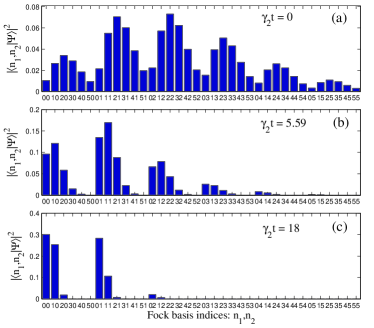
Figure 4: (Color online) We give the structure of the eigenstate of the density matrix corresponding to the maximal eigenvalue (i.e. the maximal probability) of the density matrix for three different propagation times, $\gamma_{2}t=0$ (a), $\gamma_{2}t=5.95$ (b) and $\gamma_{2}t=18$ (c). Here the abscissa is the ordered Fock basis indices $n_{1}n_{2}$ of the state amplitude. The parameters are as in Fig. 3.

The predictions were checked with the quantum Monte-Carlo simulations of the master equation (34) in the local basis $a_{1,2}$ using the “quantum jumps” method ME . The numerically obtained output density matrix indeed describes an entangled state of the two linear local modes $a_{1}$ and $a_{2}$, see Fig. 3. We use the negativity as a measure of the entanglement Negat ; Peres , but with the minus sign in front (for convenience of comparison with the smallest negative eigenvalue). It is equal to the sum of all negative eigenvalues of the partially transposed with respect to the local modes $a_{1,2}$ density matrix, $\rho^{PT}$: $\mathcal{N}(\rho)\equiv\sum_{E<0}E(\rho^{PT})$ (due to technical reasons, in calculation of the negativity the expansion over the Fock states was truncated at $n=5$, however, this turns out to be sufficient to capture negative eigenvalues FN , moreover, the higher Fock number states are populated significantly only for the relatively short time). The output density matrix turns out to be close to a pure state (for a pure input state): the largest eigenvalue of the output density matrix drops during the evolution only to $0.85$ at $\gamma_{2}t=18$ in Fig. 3. The significant elements of the corresponding eigenstate of the density matrix involve the trivial null states given by Eq. (36) and few Fock states with higher population of the local modes $a_{1,2}$, see Fig. 4. Our simulations show that this seems to be the only outcome for the output density matrix at least for small amplitudes of the coherent initial states. In view of the above arguments, this result must be expected also for arbitrary amplitudes.

V Conclusion

We have shown that it is possible to generate the nonclassical states of light by emulation of the nonlinear absorptions using the usual Kerr-nonlinearity, linear mode coupling and the strong linear losses. We have concentrated on the potential capabilities of the scheme to generate various quantum states in the simplest possible setups of three and four coupled modes. We have found that, additionally to the single-photon states, also the phase states and the entangled states can be generated by our method. It is interesting to observe, that though our scheme depends significantly on the Kerr nonlinearity (which must be present at least in one of the modes) the output states can be localized in the linear modes, as in the case of the phase states and the two-mode entangled states. Though, we have not been able to present a similar scheme for the single photon states, there is some hope that such a scheme may also exist. Having the output state localized in the linear modes of the system prevents its subsequent degradation by the destructive linear losses, accompanying any known strong Kerr nonlinearity, but quite small in the linear media. We believe that our scheme can be realized in a practical setup with the current technology. Some perspective candidates are the optical fiber coupler or the multi-core fiber, the electromagnetically induced transparency media, where the “giant” Kerr nonlinearity has been demonstrated kerr .

- (1) M. A. Nielsen and I. L. Chuang, Quantum Computation and Quantum Information (Cambridge University, Cambridge, England, 2000).
- (2) L. Mandel and E. Wolf, Optical Coherence and Quantum Optics (Cambridge University, Cambridge, England, 1995), and the references therein.
- (3) S. Kilin and D. Horoshko, Phys. Rev. Lett. 74, 5206 (1995).
- (4) S. Pezzagna, D.Rogalla, D. Wildanger, J.Meijer and A. Zaitsev, New Jornal of Physics, 13 035024 (2011).
- (5) B. Lounis and M. Orrit, Rep. Prog. Phys. 68 1129 (2005).
- (6) A. Imamoglu and Y. Yamamoto, Phys. Rev. Lett. 72, 210 (1994).
- (7) J. Kim, O. Benson, H. Kan, and Y. Yamamoto, Nature (London) 397, 500 (1999).
- (8) D. F. Walls and G. J. Milburn, Phys. Rev. A31, 4203 (1995).
- (9) A. R. R. Carvalho, P. Milman, R. L. de Matos Filho, and L. Davidovich, Phys. Rev. Lett. 86, 4988 (2001).
- (10) B. Kraus, H. P. Büchler, S. Diehl, A. Kantian, A. Micheli and P. Zoller, Phys. Rev. A 78, 042307 (2008); R. Wu, A. Pechen, C. Brif and H. Rabitz, J. Phys. A: Math. Theor. 40, 5681 (2007).
- (11) F. Verstraete, M. M. Wolf and J. I. Cirac, Nat. Phys. Lett. 5, 633 (2009).
- (12) J. F. Poyatos, J. I. Cirac and P. Zoller, Phys. Rev. Lett. 77, 4728 (1996).
- (13) D. Leibfried, R. Blatt, C. Monroe, D. Wineland, Rev. Mod. Phys. 75, 281 (2003).
- (14) I. Bloch, J. Dalibard,W. Zwerger, Rev. Mod. Phys. 80, 885 (2008).
- (15) H. Ezaki, E. Hanamura, and Y. Yamamoto, Phys. Rev. Lett. 83, 3558 (1999).
- (16) M. Alexanian, S. K. Bose, Phys. Rev. Lett. 85, 1136 (2000).
- (17) H. Ezaki, E. Hanamura, and Y. Yamamoto, Phys. Rev. Lett. 85, 1137 (2000).
- (18) T. Hong, M. W. Jack, and M. Yamashita, Phys. Rev. A 70, 013814 (2004).
- (19) D. Mogilevtsev and V. S. Shchesnovich, Optt. Lett. 35, 3375 (2010).
- (20) P. Facchi and S. Pascazio, J. Phys. A: Math. Theor. 41, 493001 (2008); P. Facchi, H. Nakazato, and S. Pascazio, Phys. Rev. Lett. 86, 2699 (2001); A.G. Kofman and G. Kurizki, Nature (London) 405, 546 (2000), Phys. Rev. Lett. 87, 270405 (2001).
- (21) K. Mølmer, Y. Castin and J. Dalibard, J. Opt. Soc. Am. B 10, 524 (1992); H. Carmichael, An Open Systems Approach to Quantum Optics (Springer, Berlin, 1993); H. P. Breuer and F. Petruccione, The Theory of Open Quantum Systems (Oxford University Press, Oxford, 2002).
- (22) M. Fleischhauer, A. Imamoglu, and J. P. Marangos, Rev. Mod. Phys. 77, 633 (2005).
- (23) V. S. Shchesnovich, D. S. Mogilevtsev, Phys. Rev. A 82, 043621 (2010).
- (24) A. Mikhalychev, D. Mogilevtsev, S. Kilin, unpublished (2011).
- (25) V. V. Dodonov and S. S. Mizrahi, Phys. Lett. A 223, 404 (1996).
- (26) A. Peres, Phys. Rev. Lett. 77, 1413 (1996).
- (27) K. Zyczkowski, P. Horodecki, A. Sanpera and M. Lewenstein, Phys. Rev. A 58, 883 (1998); G. Vidal and R. F. Werner, Phys. Rev. A 65, 032314 (2002).
- (28) This is clear from the fact that, for a Hermitian matrix, if any of the principal submatrices, i.e. consisting of the same subset of rows and columns, has negative eigenvalues, then the full matrix also has negative eigenvalues.