Integrable hierarchies and the mirror model of local $\mathbb{C}\mathbb{P}^{1}$

Abstract.

We study structural aspects of the Ablowitz-Ladik (AL) hierarchy in the light of its realization as a two-component reduction of the two-dimensional Toda hierarchy, and establish new results on its connection to the Gromov-Witten theory of local $\mathbb{C}\mathbb{P}^{1}$. We first of all elaborate on the relation to the Toeplitz lattice and obtain a neat description of the Lax formulation of the AL system. We then study the dispersionless limit and rephrase it in terms of a conformal semisimple Frobenius manifold with non-constant unit, whose properties we thoroughly analyze. We build on this connection along two main strands. First of all, we exhibit a manifestly local bi-Hamiltonian structure of the Ablowitz-Ladik system in the zero-dispersion limit. Secondarily, we make precise the relation between this canonical Frobenius structure and the one that underlies the Gromov-Witten theory of the resolved conifold in the equivariantly Calabi-Yau case; a key role is played by Dubrovin’s notion of “almost duality” of Frobenius manifolds. As a consequence, we obtain a derivation of genus zero mirror symmetry for local $\mathbb{C}\mathbb{P}^{1}$ in terms of a dual logarithmic Landau-Ginzburg model.

1. Introduction

Integrable hierarchies find a special place of appearance in moduli space problems motivated by topological field theory. A prominent case study is provided by the classical integrable hierarchies that conjecturally govern the Gromov–Witten theory of symplectic manifolds. Denote with $\overline{\mathcal{M}}_{g,n}(X,\beta)$ the stable compactification [Kontsevich:1994na] of the moduli space of degree $\beta\in H_{2}(X,\mathbb{Z})$ $J$-holomorphic maps from $n$-pointed, arithmetic genus $g$ curves to a Kähler manifold $(X,J,\omega)$. The Gromov–Witten invariants of $X$ are defined as

$$\left\langle\tau_{p_{1}}(\phi_{\alpha_{1}})\dots\tau_{p_{n}}(\phi_{\alpha_{n}})\right\rangle_{g,n,\beta}^{X}:=\int_{[\overline{\mathcal{M}}_{g,n}(X,\beta)]^{\rm vir}}\prod_{i=1}^{n}\operatorname{ev}^{*}_{i}(\phi_{\alpha_{i}})\psi_{i}^{p_{i}}$$ (1)

where $[\overline{\mathcal{M}}_{g,n}(X,\beta)]^{\rm vir}$ is the virtual fundamental class of $\overline{\mathcal{M}}_{g,n}(X,\beta)$, $\phi_{\alpha_{i}}\in H^{\bullet}(X,\mathbb{C})$ are arbitrary co-homology classes of $X$, $\operatorname{ev}_{i}:\overline{\mathcal{M}}_{g,n}(X,\beta)\to X$ is the evaluation map at the $i^{\rm th}$ marked point, and $\psi_{i}=c_{1}(\mathcal{L}_{i})$ are the first Chern classes of the universal cotangent line bundles $\mathcal{L}_{i}$ on $\overline{\mathcal{M}}_{g,n}(X,\beta)$. These numbers are interesting from a variety of points of view: in string theory, they compute worldsheet instanton effects for type IIA strings; in symplectic topology, they yield a highly sophisticated set of invariants of the symplectic structure $\omega$; in enumerative algebraic geometry, they have an interpretation as a “virtual count” of holomorphic curves inside $X$.

Kontsevich’s celebrated proof [Kontsevich:1992ti] of Witten’s conjecture [MR1068086, Witten:1990hr] relating the Korteweg–de Vries hierarchy to intersection theory on the Deligne–Mumford moduli space of curves $\overline{\mathcal{M}}_{g,n}$ suggested a connection between Gromov–Witten theory and integrable systems in the following form. Let $\epsilon$ and $t^{\alpha,p}$ be formal symbols, where $\alpha=\{1,\dots,h_{X}\}$, $h_{X}:=\dim_{\mathbb{C}}H^{\bullet}(X,\mathbb{C})$ and $p\in\mathbb{N}$, and denote with $\mathbf{t}$ the set $\mathbf{t}:=\left\{t^{\alpha,p}\right\}_{\begin{subarray}{c}\alpha\in h_{X}\\ p\in\mathbb{N}\end{subarray}}$. Write $\phi_{1}$ for the identity of $H^{\bullet}(X)$ and define $x:=t^{1,0}$. The all-genus, full-descendant Gromov–Witten potential of $X$ is the formal power series

$$\mathcal{F}^{X}(\epsilon,\mathbf{t})=\sum_{g\geq 0}\epsilon^{2g-2}\sum_{\beta\in H_{2}(X,\mathbb{Z})}\sum_{n\geq 0}\sum_{p_{1},\ldots,p_{n}}{\prod_{i=1}^{n}t^{\alpha_{i},p_{i}}\over n!}\left\langle\tau_{p_{1}}(\phi_{\alpha_{1}})\dots\tau_{p_{n}}(\phi_{\alpha_{n}})\right\rangle_{g,n,\beta}^{X}.$$ (2)

We then have the following

Conjecture 1.1.

Let $\mathcal{F}^{X}(\epsilon,\mathbf{t})$ denote the all-genus full descendant Gromov-Witten potential of $X$. Then there exists a Hamiltonian integrable hierarchy of PDEs such that $\epsilon^{2}\mathcal{F}^{X}(\epsilon,\mathbf{t})$ is the logarithm of a $\tau$–function associated with one of its solutions. The variables $t^{\alpha,p}$ are identified with times of the hierarchy, and the genus counting variable $\epsilon$ with a perturbative parameter in a small dispersion expansion of the equations.

The case $X=\{\mathrm{pt}\}$ is the statement of the Witten–Kontsevich theorem. This connection has provided a mutually fruitful source of insights for the integrable systems community on one hand, and for symplectic and algebraic geometers on the other.

After the Witten–Kontsevich theorem, a lot of effort has been put to further elucidate the origin of integrability in Gromov–Witten theory, and to find constructuve proofs of Conjecture 1.1 for more general target spaces. Research in this direction has received much attention in the early 90’s, starting from the discovery by Dubrovin and Krichever of a clear link between topological Landau–Ginzburg models and the hydrodynamics of weakly deformed soliton lattices [Krichever:1992qe, Dubrovin:1992eu]. Subsequently, the field gained further momentum from Dubrovin’s systematic study of WDVV equations [MR1068086, Dijkgraaf:1990qw] and his universal construction [Dubrovin:1992dz], for arbitrary homogeneous chiral algebras, of dispersionless (bi-)Hamiltonian integrable hierarchies that encode the descendent sector of the theory - namely, in the case of quantum co-homologies, the complete set of descendent genus zero Gromov–Witten invariants.
In more recent times, the (hard) task of incorporating dispersive corrections in the picture - corresponding, in the original Witten-Kontsevich picture, to higher genus Gromov–Witten invariants - has followed two main strands. On one hand, the Dubrovin–Zhang program of classification of normal forms of bi-Hamiltonian evolutionary hierarchies has provided a concrete incarnation of Virasoro constraints from the integrable system point of view, along with a complete reconstruction theorem for higher genus descendent invariants [dubrovin-2001]; on the other, generalizations of the Witten–Kontsevich correspondence were explicitly constructed for the quantum co-homology of simple target orbifolds, such as $BG$ [MR1950944] and $[\mathbb{CP}^{1}/G]$ [MR2199226, MR2433616, pauljohnsonthesis, rossi-2008].

1.1. The resolved conifold and the Ablowitz–Ladik hierarchy

Inspired by the appearance of trilogarithmic prepotentials in Dubrovin’s study of the Ablowitz–Ladik (AL) hierarchy [MR2462355], one of us proposed in [Brini:2010ap] that Conjecture 1.1 should hold true when $X$ is a particular local Calabi-Yau manifold of dimension three – the resolved conifold – given by the strict transform of the nodal quadric in $\mathbb{A}^{4}$, and the corresponding integrable hierarchy is the Ablowitz–Ladik hierarchy [MR0377223]. The precise statement, which was proven in [Brini:2010ap] at the first few orders in the genus expansion, relates a peculiar form of the AL hierarchy to the Gromov-Witten theory of $\mathcal{O}_{\mathbb{P}^{1}}(-1)_{[\nu]}\oplus\mathcal{O}_{\mathbb{P}^{1}}(-1)_{[-\nu]}$, equivariant with respect to a fiber-wise $T\simeq\mathbb{C}^{*}$-action which covers the trivial action on the base $\mathbb{P}^{1}$ and rotates the fibers with opposite weights; we denoted with $\nu$ the first Chern class of the line bundle $\mathcal{O}(1)\to BT\simeq\mathbb{C}\mathbb{P}^{\infty}$. Restricting to genus zero, primary invariants, this statement can be rephrased as the equality of the quantum co-homology ring of the resolved conifold in the equivariantly Calabi-Yau case with the Frobenius structure that arises from a particular solution of WDVV, first encountered in the treatment of the AL system in [MR2462355].

This example, which is of remarkable importance in the Gromov–Witten theory of Calabi-Yau threefolds, raised various interesting questions: among them, the possibility to provide a local mirror symmetry construction for this equivariant case, and the explanation of the apparent breakdown of bi-Hamiltonianity on the integrable system side. In this paper we study both aspects in detail, by regarding the AL hierarchy as the Toeplitz reduction of 2D-Toda [MR1794352, MR1993935, MR2534519]. We first of all build, in Section 2, on the identification of the AL lattice with the Toeplitz lattice and provide a clean proof of the invariance of the Toeplitz condition under the 2D-Toda flows at the dispersive level in the bi-infinite case. By observing that the Toeplitz Lax matrices admit a factorization in terms of two bi-diagonal matrices, we show that the Toeplitz lattice is an instance of rational reduction of the 2D-Toda hierarchy, which can be defined in general by analogy with the rational reductions of KP hierarchy [MR1340299, MR1352392]. We then apply the dispersionless Lax formalism of 2D-Toda to associate a new, canonical Frobenius structure with the hierarchy. This new Frobenius manifold is different from the one that appears in Gromov–Witten theory: it fails to have a covariantly constant unit vector field, but it satisfies all the other axioms of a Frobenius manifold, including somewhat surprisingly the existence of a linear Euler vector field. In particular, this entails the existence of a local bi-Hamiltonian structure of Dubrovin–Novikov type [MR1037010], to be contrasted with the inhomogeneity of the prepotentials in [MR2462355, Brini:2010ap] and the non–locality of the pairs constructed in [MR2238744].
A natural question that arises is then how this new Frobenius structure and the quantum co-homology of the resolved conifold are related to one another. We find in Section 3 that the relation in question is remarkably given in the form of Dubrovin’s almost duality of Frobenius manifolds [MR2070050]. By pushing the dispersionless Lax formalism through the duality we obtain a logarithmic Landau–Ginzburg mirror for local $\mathbb{CP}^{1}$, close in form to the LG models proposed by Hori, Iqbal and Vafa for the non-equivariant theory [Hori:2000ck]. We finally study the period structure of the resulting almost Frobenius manifold, and find a remarkable connection to the theory of singularities of divisors considered in the context of twisted Picard–Lefschetz theory by Givental in [MR936695]. We conclude in Section 4 with remarks on open problems and new avenues of research.

Acknowledgements.

It is a privilege to dedicate this work to Boris Dubrovin, for his guidance during our PhD years in Trieste and for the many enlightening (and fun!) discussions we have had with him over the last few years. We would moreover like to thank M. Cafasso, I. Krichever, P. Lorenzoni, F. Magri and all the participants of the conference on “Integrable Systems in Pure and Applied Mathematics” at Alghero, June 2010, for discussions and their interest in this project. We would also like to thank the Complex Geometry Group of Université Paris VI, the Departments of Mathematics of the Universities of Geneva, Glasgow and Milano-Bicocca, and in particular G. Falqui, X. Ma, I. Strachan and A. Szenes for kind hospitality while this work was being prepared. A. B. was supported by a Postdoctoral Fellowship of the Swiss National Science Foundation (FNS); partial support from the INdAM-GNFM Grant “Teoria di stringa topologica e sistemi integrabili” is also acknowledged. G. C. wishes to acknowledge the support of the Center for Mathematics of the University of Coimbra (CMUC), the Mathematical Physics sector of SISSA in Trieste and the Mathematics Department of University of Milano-Bicocca. P. R. was supported by a Postdoc of Fondation de Sciences Mathématiques de Paris at the Institut de Mathématiques de Jussieu, UPMC, Paris 6.

2. Ablowitz-Ladik and $2D$-Toda hierarchies

2.1. Ablowitz-Ladik system and Toeplitz lattice

The complexified Ablowitz-Ladik (AL) system [MR0377223] is given by the pair of equations

$$\dot{x}_{n} = \frac{1}{2}(1-x_{n}y_{n})(x_{n-1}+x_{n+1}),$$

$$\dot{y}_{n} = -\frac{1}{2}(1-x_{n}y_{n})(y_{n-1}+y_{n+1})$$ (3)

defining the time evolution of two sequences of complex variables $x_{n}$, $y_{n}$ with $n\in\mathbb{Z}$. The AL system admits an infinite number of conservation laws and is part of a hierarchy of mutually commuting evolutionary flows, usually described by semidiscrete zero-curvature equations [MR0377223, MR1993935].

In the semi-infinite case the AL hierarchy is equivalent, as noted in [MR1794352, MR1993935] and shown in detail by Cafasso [MR2534519], to a peculiar reduction of the 2D-Toda lattice hierarchy, called the Toeplitz lattice, which naturally arises in the study of the integrable dynamics of moment matrices associated with biorthogonal polynomials on the unit circle and whose orbits are selected by Toeplitz initial data for an associated factorization problem [MR0810626]. In particular it describes the solution associated with a unitary matrix model [MR1794352].

Rather than dealing with the semi-infinite case, we present here a slightly more general definition of the Toeplitz lattice in the case of bi-infinite matrices, i.e. we assume that the matrix indices below span integer values, $n,m\in\mathbb{Z}$. This choice turns out to be somehow more natural, allowing us to easily identify the Toeplitz lattice with a rational reduction of the 2D-Toda hierarchy and to obtain the dispersionless limit that we need later. The semi-infinite case will be recovered as a further simple reduction (see Appendix A for further details of this analysis in the case of the semi-infinite Toeplitz lattice).

Recall that the 2D-Toda Lax matrices [MR810623] are given by

$$L_{1}=\Lambda+\sum_{j\leq 0}u^{(1)}_{j}\Lambda^{j},\qquad L_{2}=u^{(2)}_{-1}\Lambda^{-1}+\sum_{j\geq 0}u^{(2)}_{j}\Lambda^{j}$$ (4)

where $\Lambda$ is the shift matrix

$$\Lambda_{n,m}=\delta_{n+1,m},$$ (5)

the diagonal matrices $u_{j}^{(i)}$ represent the dependent variables and the matrix indices $n,m\in\mathbb{Z}$. The 2D-Toda flows can be written in the Lax form as

$$\partial_{s^{(1)}_{j}}L_{i}=\left[\left(L_{1}^{j}\right)_{+},L_{i}\right],\quad\partial_{s^{(2)}_{j}}L_{i}=\left[\left(L_{2}^{j}\right)_{-},L_{i}\right],\qquad i=1,2$$ (6)

where we denoted by $M_{+}$ (resp. $M_{-}$) the upper (resp. lower) diagonal part of a matrix $M$, including (resp. excluding) the main diagonal.

Definition 2.1.

We say that $L_{1}$ and $L_{2}$ are Toeplitz Lax matrices if they can be written in the form

$$L_{1}=\left(\begin{array}[]{ccc|ccccc}\ddots&&&&&&\\ &-x_{-1}y_{-2}&1&0&0&0&\\ &-v_{-1}x_{0}y_{-2}&-x_{0}y_{-1}&1&0&0&\\ \hline\cr&-v_{-1}v_{0}x_{1}y_{-2}&-v_{0}x_{1}y_{-1}&-x_{1}y_{0}&1&0&\\ &-v_{-1}v_{0}v_{1}x_{2}y_{-2}&-v_{0}v_{1}x_{2}y_{-1}&-v_{1}x_{2}y_{0}&-x_{2}y_{1}&1&\\ &-v_{-1}v_{0}v_{1}v_{2}x_{3}y_{-2}&-v_{0}v_{1}v_{2}x_{3}y_{-1}&-v_{1}v_{2}x_{3}y_{0}&-v_{2}x_{3}y_{1}&-x_{3}y_{2}&\\ &&&&&&\ddots\end{array}\right),$$ (7a)

$$L_{2}=\left(\begin{array}[]{ccc|ccccc}\ddots&&&&&&\\ &-x_{-2}y_{-1}&-x_{-2}y_{0}&-x_{-2}y_{1}&-x_{-2}y_{2}&-x_{-2}y_{3}&\\ &v_{-1}&-x_{-1}y_{0}&-x_{-1}y_{1}&-x_{-1}y_{2}&-x_{-1}y_{3}&\\ \hline\cr&0&v_{0}&-x_{0}y_{1}&-x_{0}y_{2}&-x_{0}y_{3}&\\ &0&0&v_{1}&-x_{1}y_{2}&-x_{1}y_{3}&\\ &0&0&0&v_{2}&-x_{2}y_{3}&\\ &&&&&&\ddots\end{array}\right)$$ (7b)

where $x_{n}$, $y_{n}\in\mathbb{C}$, $n\in\mathbb{Z}$ and $v_{n}:=1-x_{n}y_{n}$.

We will prove shortly that this is indeed a symmetry reduction of the 2D-Toda lattice.

It is convenient to write these matrices in the equivalent form

$$L_{1} =\Lambda-x^{+}\left(1-(1-xy)\Lambda^{-1}\right)^{-1}y,$$ (8a)

$$L_{2} =(1-xy)\Lambda^{-1}-x\left(1-\Lambda\right)^{-1}y^{+}$$ (8b)

where $x$, resp. $y$, are diagonal matrices with entries given by $x_{n}$, resp. $y_{n}$, and $x^{+}$ denotes the shifted variable $x$, $\Lambda x=x^{+}\Lambda$.

Here and in the following the formal inverse of a matrix of the form $1-X$ is given by geometric series in $X$ and for this reason we sometimes denote it with $\frac{1}{1-X}$. Note that this is a proper (left and right) inverse of the bi-diagonal matrix $1-X$ with respect to the usual matrix multiplication.

Note that we can also write

$$L_{1}=\Lambda\frac{1}{v}\left(1-x\frac{1}{1-v\Lambda^{-1}}y\right),\quad L_{2}=\left(1-x\frac{1}{1-\Lambda}y\right)\Lambda^{-1}.$$ (9)

One can easily recognize $L_{2}$ to be a simple extension to the bi-infinite case of the semi-infinite version given in [MR1794352]. On the other hand $L_{1}$ is usually given in a dressed form. To see this, let $\ell$ be a diagonal matrix

$$\ell=\operatorname{diag}\left(\dots,\ell_{-1},\ell_{0},\ell_{1},\dots\right)$$ (10)

with entries that satisfy

$$\frac{\ell_{n+1}}{\ell_{n}}=1-x_{n+1}y_{n+1},\qquad n\in\mathbb{Z}.$$ (11)

Then

Lemma 2.1.

We have

$$\ell^{-1}L_{1}\ell=\Lambda\left(1-x\frac{1}{1-\Lambda^{-1}}y\right)$$

where $(1-\Lambda^{-1})^{-1}$ is given by the matrix $\sum_{k\geq 0}\Lambda^{-k}$.

Proof.

A simple computation, rewriting (11) as

$$\ell\Lambda\ell^{-1}=\Lambda\frac{1}{1-xy},\qquad\ell\Lambda^{-1}\ell^{-1}=(1-xy)\Lambda^{-1}.$$

∎

Explicitly

$$\ell^{-1}L_{1}\ell=\left(\begin{array}[]{ccc|ccccc}\ddots&&&&&&\\ &-x_{-1}y_{-2}&v_{-1}&0&0&0&\\ &-x_{0}y_{-2}&-x_{0}y_{-1}&v_{0}&0&0&\\ \hline\cr&-x_{1}y_{-2}&-x_{1}y_{-1}&-x_{1}y_{0}&v_{1}&0&\\ &-x_{2}y_{-2}&-x_{2}y_{-1}&-x_{2}y_{0}&-x_{2}y_{1}&v_{2}&\\ &-x_{3}y_{-2}&-x_{3}y_{-1}&-x_{3}y_{0}&-x_{3}y_{1}&-x_{3}y_{2}&\\ &&&&&&\ddots\end{array}\right)$$

which is the obvious extension of $\ell^{-1}L_{1}\ell$ appearing in the semi-infinite Toeplitz lattice.

We now show that the form of these matrices is preserved by 2D-Toda flows and that they correspond to the simplest rational reduction. This follows from two simple observations.

Proposition 2.2.

The Lax operators $L_{i}$ can be factorized as

$$L_{1}=AB^{-1},\qquad L_{2}=BA^{-1}$$ (12)

where the bi-diagonal matrices $A$ and $B$ are given by

$$A=-\frac{1}{y^{+}}(1-\Lambda)y,\qquad B=\frac{1}{y}(1-v\Lambda^{-1})y.$$ (13)

Proof.

A simple computation, in the case of $L_{2}$

$$BA^{-1} =-\frac{1}{y}\left(1-v\Lambda^{-1}\right)\left(1-\Lambda\right)^{-1}y^{+}$$

$$=\frac{1}{y}\left(v\Lambda^{-1}(1-\Lambda)-xy\right)(1-\Lambda)^{-1}y^{+}$$

$$=\frac{v}{y}\Lambda^{-1}y^{+}-x(1-\Lambda)^{-1}y^{+}$$

that is equal to (8b). Notice that in the second equality we have used the identity $\Lambda^{-1}\Lambda=1$, which is not satisfied in the semi-infinite case. ∎

Explicitly

$$A=\left(\begin{array}[]{cc|ccc}\ddots&&&&\\ &-\frac{y_{-1}}{y_{0}}&1&0&\\ \hline\cr&0&-\frac{y_{0}}{y_{1}}&1&\\ &0&0&-\frac{y_{1}}{y_{2}}&\\ &&&&\ddots\end{array}\right),\quad B=\left(\begin{array}[]{ccc|cc}\ddots&&&&\\ &-v_{-1}\frac{y_{-2}}{y_{-1}}&1&0&\\ \hline\cr&0&-v_{0}\frac{y_{-1}}{y_{0}}&1&\\ &0&0&-v_{1}\frac{y_{0}}{y_{1}}&\\ &&&&\ddots\end{array}\right).$$

We prove that rational Lax matrices (12) are invariant under the 2D-Toda flows following an argument similar to that of [MR1340299] for the rational reductions of the KP hierarchy.

Proposition 2.3.

Given infinite matrices of the form

$$A=\Lambda+a,\quad B=1+b\Lambda^{-1}$$ (14)

for diagonal matrices $a$, $b$, the equations

$$A_{s^{(1)}_{i}}=((AB^{-1})^{i})_{+}A-A((B^{-1}A)^{i})_{+},\quad B_{s^{(1)}_{i}}=((AB^{-1})^{i})_{+}B-B((B^{-1}A)^{i})_{+},$$ (15a)

$$A_{s^{(2)}_{i}}=((BA^{-1})^{i})_{-}A-A((A^{-1}B)^{i})_{-},\quad B_{s^{(2)}_{i}}=((BA^{-1})^{i})_{-}B-B((A^{-1}B)^{i})_{-}$$ (15b)

are well-defined and induce the 2D-Toda equations (6) on the Lax operators (12).

Proof.

Let us check the first equation in  (15a). Clearly the right-hand side is upper triangular. Rewriting it as

$$A((B^{-1}A)^{i})_{-}-((AB^{-1})^{i})_{-}A$$

one concludes that it is actually diagonal, hence the equation is well-defined. ∎

2.2. Hamiltonian formalism and dispersionless limit

The bi-infinite Toeplitz flows can be cast in Hamiltonian form

$$\frac{\partial x_{n}}{\partial s^{(k)}_{i}}=(1-x_{n}y_{n})\frac{\partial H^{(k)}_{i}}{\partial y_{n}}, \frac{\partial y_{n}}{\partial s^{(k)}_{i}}=-(1-x_{n}y_{n})\frac{\partial H^{(k)}_{i}}{\partial x_{n}}$$ (16)

where the Hamiltonians

$$H^{(k)}_{i}:=-\frac{1}{i}\operatorname{Tr}~{}{L}_{k}^{i},~{}~{}i=1,2,3,...,~{}~{}k=1,2$$ (17)

mutually commute with respect to the symplectic structure

$$\omega:=\sum_{k\in\mathbb{Z}}\frac{dx_{k}\wedge dy_{k}}{1-x_{k}y_{k}}.$$ (18)

The first equations of the hierarchy, i.e. the Ablowitz-Ladik system (3), correspond to the combination of Hamiltonians

$$H_{AL}:=\frac{1}{2}(H_{1}^{(1)}+H_{1}^{(2)})=-\frac{1}{2}\operatorname{Tr}~{}\left(L_{1}+L_{2}\right)=\frac{1}{2}\sum_{i\in\mathbb{Z}}\left(x_{i+1}y_{i}+x_{i}y_{i+1}\right).$$

To conclude our treatment of the Toeplitz lattice as rational 2D-Toda reduction we prove that

Proposition 2.4.

The Hamilton equations (16) induce on the matrices (13) the flows (15).

Proof.

As noted in previous proof, both sides of the first equation in (15a) are diagonal, hence it can be written

$$\frac{\partial}{\partial s_{i}^{(1)}}\left(\frac{y_{n}}{y_{n+1}}\right)=\frac{y_{n}}{y_{n+1}}\left((AB^{-1})^{i}-(B^{-1}A)^{i}\right)_{n,n}.$$ (19)

On the other hand the Hamilton equations (16) give

$$\frac{\partial}{\partial s_{i}^{(1)}}\left(\frac{y_{n}}{y_{n+1}}\right)=\frac{y_{n}}{y_{n+1}}\left(-\frac{v_{n}}{y_{n}}\frac{\partial H_{i}^{(1)}}{\partial x_{n}}+\frac{v_{n+1}}{y_{n+1}}\frac{\partial H_{i}^{(1)}}{\partial x_{n+1}}\right).$$ (20)

We need to check that (20) implies (19). Using the fact that $L_{1}=AB^{-1}$ and that $A$ does not depend on $x_{n}$ we can compute

$$\frac{\partial H_{i}^{(1)}}{\partial x_{n}}=(y^{-}\Lambda^{-1}B^{-1}L_{1}^{i})_{n,n}$$

and

$$-\frac{v_{n}}{y_{n}}\frac{\partial H_{i}^{(1)}}{\partial x_{n}}=-\left(\frac{vy^{-}}{y\ }\Lambda^{-1}B^{-1}L_{1}^{i}\right)_{n,n}=\left((AB^{-1})^{i}\right)_{n,n}-\left(B^{-1}(AB^{-1})^{i}\right)_{n,n},$$ (21)

where, in the last equality, we have used the identity

$$-\frac{vy^{-}}{y\ }\Lambda^{-1}=B-1$$

which follows from (13). Similarly

$$\frac{v_{n+1}}{y_{n+1}}\frac{\partial H_{i}^{(1)}}{\partial x_{n+1}} =\left(\frac{vy^{-}}{y\ }\Lambda^{-1}B^{-1}L_{1}^{i}\right)_{n+1,n+1}$$

$$=\left(B^{-1}L_{1}^{i}\frac{vy^{-}}{y\ }\Lambda^{-1}\right)_{n,n}$$ (22)

$$=-\left((B^{-1}A)^{i}\right)_{n,n}+\left(B^{-1}(AB^{-1})^{i}\right)_{n,n}.$$

Substituting (21) and (22) in (20) we conclude. The rest of the equations (15) are obtained from the Hamilton equations with analogous computations which we leave as an exercise to the reader. ∎

Remark 2.5.

We already mentioned that the multiplication might not be associative in the case of infinite matrices. Indeed, from the factorization (12) one is tempted to conclude that $L_{1}L_{2}=(AB^{-1})(BA^{-1})$ equals, assuming associativity, to $A(B^{-1}B)A^{-1}=1$. However it is easy to check from (7) that $L_{1}L_{2}\not=1\not=L_{2}L_{1}$. A version of this constraint will nonetheless work in semi-infinite case.

In view of the last remark, it is worth to point out that the semi-infinite Toeplitz lattice departs slightly from the bi-infinite case, and it is interesting to investigate on its own especially in view of its connection to unitary matrix models [MR1794352]. We give the details of this case in Appendix A.

Following [MR2462355], we introduce the pair of variables

$$\begin{split}w&=\log\left(1-xy\right),\\ v&=\frac{1}{2}\left(1-\Lambda^{-1}\right)(\log x-\log y).\end{split}$$ (23)

With this choice of dependent variables, the Lax matrices can be rewritten as

$$\begin{split}L_{1}&=\Lambda\mathrm{e}^{-w}\left(1-\sqrt{1-\mathrm{e}^{w}}\frac{1}{1-\mathrm{e}^{v+w}\Lambda^{-1}}\sqrt{1-\mathrm{e}^{w}}\right),\\ L_{2}&=\left(1-\sqrt{1-\mathrm{e}^{w}}\frac{1}{1-\Lambda\mathrm{e}^{-v}}\sqrt{1-\mathrm{e}^{w}}\right)\Lambda^{-1}.\end{split}$$ (24)

In this case

$$L_{1}=AB^{-1},\quad L_{2}=BA^{-1}$$

for

$$A=-\frac{\mathrm{e}^{v^{+}}}{\sqrt{1-\mathrm{e}^{w^{+}}}}\left(1-\mathrm{e}^{-v^{+}}\Lambda\right),\quad B=\frac{1}{\sqrt{1-\mathrm{e}^{w}}}\left(1-\mathrm{e}^{v+w}\Lambda^{-1}\right).$$

These matrices can be alternatively seen as formal difference operators acting on the real line and, correspondingly, the dependent variables $v$ and $w$ as functions of a space variable $x$ (not to be confused with the dependent variable denoted above with the same symbol).

This observation allows us to straightforwardly obtain the long-wave limit of the Toeplitz lattice in Lax form. The symbols of the Lax operators [MR1346289]

$$\lambda_{i}(p)=\sigma_{L_{i}}(p),\quad i=1,2$$

are given by rational functions

$$\lambda_{1}(p)=p\left(\frac{p-\mathrm{e}^{v}}{p-\mathrm{e}^{v+w}}\right)=(\lambda_{2}(p))^{-1},$$ (25)

hence the dispersionless Lax equations can be compactly written in terms of the Lax symbol $\lambda(p):=\lambda_{1}(p)$ as

$$\frac{\partial\lambda}{\partial s^{(1)}_{n}}=\{\left(\lambda^{n}\right)_{+},\lambda\}_{[L]},\quad\frac{\partial\lambda}{\partial s^{(2)}_{n}}=\{\left(\lambda^{-n}\right)_{-},\lambda\}_{[L]},\quad i=1,2\quad,$$ (26)

where $()_{\pm}$ denote the projections to the analytic and principal part and the Poisson bracket $\{,\}_{[L]}$ is defined as

$$\{a(p,x),b(p,x)\}_{[L]}:=p\frac{\partial a(p,x)}{\partial p}\frac{\partial b(p,x)}{\partial x}-p\frac{\partial a(p,x)}{\partial x}\frac{\partial b(p,x)}{\partial p}.$$ (27)

2.3. A conformal Frobenius manifold for the AL hierarchy

The dispersionless Lax formalism for the Toeplitz reduction of 2D-Toda paves the way to canonically associate a Frobenius manifold with the AL hierarchy. We denote by $M_{g;n_{1},\dots,n_{m}}$ the Hurwitz space

$$M_{g;n_{1},\dots,n_{m}} =\big{\{} (\Gamma;p_{1},\dots,p_{m};f):\Gamma\hbox{ smooth projective, }\dim_{\mathbb{C}}\Gamma=1,h^{1,0}(\Gamma)=g,$$ (28)

$$f:\Gamma\to\mathbb{C}\mathbb{P}^{1}\in\mathcal{O}_{\Gamma\setminus\{p_{1},\dots,p_{m}\}},e_{f}(p_{j})=n_{j}\big{\}}/\mathord{\sim}$$

where the quotient is under biholomorphic equivalence. We can view the dispersionless Lax operator

$$\lambda(p)=p+\mathrm{e}^{v}(\mathrm{e}^{w}-1)+\mathrm{e}^{2v+w}\frac{\mathrm{e}^{w}-1}{p-\mathrm{e}^{v+w}}$$ (29)

as the datum of a degree 2 covering map $\lambda:\mathbb{C}\mathbb{P}^{1}\to\mathbb{C}\mathbb{P}^{1}$ which is unramified at infinity, that is, $[(\lambda(p),\mathbb{C}\mathbb{P}^{1})]/\mathord{\sim}\in M_{0;1,1}$, where we pick an equivalence class under Möbius transformation in the form (29). We have in this case

$$p_{1}=\infty,\quad p_{2}=\mathrm{e}^{v+w}.$$ (30)

By regarding (29) as the tree-level superpotential of a topological Landau-Ginzburg model [Dubrovin:1992eu, Dubrovin:1994hc, Krichever:1992qe], we can associate a Frobenius structure with $M_{0;1,1}$ as follows. Let $[\Gamma,f]\in M_{g,n_{1},\dots,n_{m}}$, $0<D<\sum_{i=1}^{m}n_{i}p_{i}$ a divisor on $\Gamma$ and $\mathrm{d}\omega\in H^{1,0}_{\bar{\partial}}(\Gamma\setminus D)$ a meromorphic differential, possibly with poles at $p_{i}$ of orders less than $n_{i}+1$. The pair $(M_{g;n_{1},\dots n_{m}},\mathrm{d}\omega)$ can be endowed with the structure of a Frobenius manifold through the Landau-Ginzburg formulae [Cecotti:1992rm, Dubrovin:1994hc]

$$\eta(\partial_{i},\partial_{j}) = \sum\mathrm{Res}_{\mathrm{d}\lambda=0}\left\{\frac{\partial_{i}\lambda(p)\partial_{j}\lambda(p)}{\lambda^{\prime}(p)}\frac{\mathrm{d}p}{p^{2}}\right\}$$ (31)

$$c(\partial_{i},\partial_{j},\partial_{k}) = \sum\mathrm{Res}_{\mathrm{d}\lambda=0}\left\{\frac{\partial_{i}\lambda(p)\partial_{j}\lambda(p)\partial_{k}\lambda(p)}{\lambda^{\prime}(p)}\frac{\mathrm{d}p}{p^{2}}\right\}$$ (32)

In order for $(M_{g;n_{1},\dots n_{m}},\mathrm{d}\omega)$ to satisfy all axioms of a Frobenius manifold, $\mathrm{d}\omega$ should fall in one of five different categories of meromorphic 1-forms, which were characterized in detail in [Dubrovin:1992eu, Dubrovin:1994hc]; such 1-differentials go under the name of admissible primary differentials. We refer the reader to [Dubrovin:1994hc] for more details, and concentrate on the case of $M_{0;1,1}$ in the following.
For the case of $M_{0;1,1}$, Dubrovin’s classification reduces to one case: $\mathrm{d}\omega$ is the unique meromorphic third kind differential with

$$\mathrm{Res}_{p=p_{1}}\mathrm{d}\omega=1,\quad\mathrm{Res}_{p=p_{2}}\mathrm{d}\omega=-1,$$ (33)

i.e., when $p_{1}=\infty$,

$$\mathrm{d}\omega=\left\{\begin{array}[]{ccc}\frac{p\mathrm{d}p}{p_{2}(p-p_{2})}&\mathrm{for}&p_{2}\neq 0\\ -\frac{\mathrm{d}p}{p}&\mathrm{for}&p_{2}=0\end{array}\right.$$ (34)

In this case, the Frobenius manifold induced by (31), (32) is the one associated with the Extended Toda hierarchy [MR2108440], which is in turn related to the Gromov-Witten theory of the projective line. In our case, the Toeplitz reduction of 2D-Toda (56) binds us to take as primitive form

$$\mathrm{d}\omega=\frac{\mathrm{d}p}{p}$$ (35)

which is not admissible; as a consequence, moving from 1D-Toda to AL implies that the solution of WDVV associated with (31), (32) will not satisfy all axioms of a Frobenius manifold. With a slight abuse of language, we will sometimes refer to this weaker structure induced on $M_{0;1,1}$ still as a “Frobenius manifold”.

This section is devoted to a thorough characterization of this canonical Frobenius structure associated with the AL hierarchy. We have the following

Theorem 2.6.

Eq. (31), (32) endow the Hurwitz space $M_{0;1,1}$ with the structure of a charge $d=1$, non-degenerate, semi-simple Frobenius manifold $\mathcal{M}_{AL}:=(M_{0;1,1},e,E,\eta,F_{0})$ with a non-covariantly constant unit $e$. In flat co-ordinates $t_{1}$, $t_{2}$ for the metric $\eta$, the prepotential reads

$$F_{0}=\frac{1}{2}t_{2}t_{1}^{2}+\mathrm{e}^{t_{2}}t_{1}+\frac{1}{2}t_{1}^{2}\log t_{1}$$ (36)

whereas the unit $e$ and the Euler vector field $E$ are given as

$$e = \frac{t_{1}\partial_{t_{1}}-t_{2}}{t_{1}-\mathrm{e}^{t_{2}}},$$ (37)

$$E = t_{1}\partial_{t_{1}}+t_{2}.$$ (38)

Proof. The proof follows from a straightforward calculation from (31), (32). We reproduce here the main steps.

It is immediate to check that the metric $\eta$ is flat. Introducing co-ordinates $(t_{1},t_{2})$ such that

$$\mathrm{e}^{v}=\mathrm{e}^{t_{2}}-t_{1},\quad w=t_{2}-\log(\mathrm{e}^{t_{2}}-t_{1}),$$ (39)

the metric $\eta$ takes the off-diagonal form

$$\eta\left(\partial_{t_{i}},\partial_{t_{j}}\right)=\delta_{i+j,3}.$$ (40)

In this co-ordinates, the Landau-Ginzburg formula (32) for the structure constants yields the expression (36) for the prepotential.

As for the usual theory of Frobenius structures on Hurwitz spaces, the critical values of the superpotential give a set of canonical co-ordinates of the Frobenius manifold. Denoting by $q_{1,2}$ the critical points of $\lambda(p)$,

$$q_{1} = \mathrm{e}^{\frac{t_{2}}{2}}\left(\mathrm{e}^{\frac{t_{2}}{2}}+\sqrt{t_{1}}\right),$$

$$q_{2} = \mathrm{e}^{\frac{t_{2}}{2}}\left(\mathrm{e}^{\frac{t_{2}}{2}}-\sqrt{t_{1}}\right),$$ (41)

canonical co-ordinates are given as

$$u_{1} = \lambda(q_{1})=\left(\mathrm{e}^{\frac{t_{2}}{2}}+\sqrt{t_{1}}\right)^{2},$$

$$u_{2} = \lambda(q_{2})=\left(\mathrm{e}^{\frac{t_{2}}{2}}-\sqrt{t_{1}}\right)^{2},$$ (42)

and it is straightforward to check that the corresponding vector fields give idempotents of the algebra (32)

$$\partial_{\gamma}uc^{\gamma}_{\alpha\beta}=\partial_{\alpha}u\partial_{\gamma}u.$$ (43)

In particular, the Frobenius algebra induced on the tangent bundle of $M_{0;1,1}$ is generically semi-simple.

With this ingredients at hand, we can readily determine the expression for the unit $e$ and the Euler vector field $E$. By definition, we have

$$e=\partial_{u_{1}}+\partial_{u_{2}}$$ (44)

and (42) implies (37). On the other hand, we know that in the usual theory of Frobenius manifolds associated with Hurwitz spaces, the vector

$$E:=\sum_{i=1,2}u_{i}\partial_{u_{i}}$$ (45)

is the Euler vector field of the Frobenius manifold. For the case at hand, (45) becomes, in flat co-ordinates

$$E=t_{1}\partial_{t_{1}}+\partial_{t_{2}}.$$ (46)

This is indeed the Euler vector field for the solution of WDVV (36). Up to quadratic terms, we have explicitly

$$L_{E}F_{0}=2F_{0}=(3-1)F_{0},$$ (47)

namely, the Frobenius structure is quasi-homogeneous, with charge $d=1$. Its non-degeneracy

$$[e,E]=e$$ (48)

follows trivially from (37), (38). ∎

Remark 2.7.

As compared to the classical definition of a Frobenius manifold, we see that the axiom of covariant constancy of the unit vector field with respect to the Levi-Civita connection of $\eta$

$$\nabla e=0$$ (49)

is violated by (36). In particular

$$\partial_{\alpha}\partial_{\beta}L_{e}F_{0}\neq\eta_{\alpha\beta}$$ (50)

Somewhat remarkably, though, the grading axiom, which states that the Euler vector field is linear

$$\nabla\nabla E=0$$ (51)

is instead respected, as is manifest from (38).

2.4. Bi-Hamiltonian structure

Denote by $\{,\}_{i}$, $i=1,2$ the Poisson brackets of hydrodynamic type on the loop space $\mathcal{L}(\mathcal{M}_{AL})$ associated with the metric $\eta$ and the intersection form $g$ respectively. Recall that the intersection form is the bilinear pairing on the cotangent bundle $T^{*}\mathcal{M}_{AL}$ defined by

$$g(w_{1},w_{2}):=i_{E}(w_{1}\cdot w_{2})$$ (52)

where the product of the $1$-forms $w_{i}$ is induced on $T^{*}\mathcal{M}_{AL}$ by the Frobenius algebra on the tangent by the map $\eta:T\mathcal{M}_{AL}\rightarrow T^{*}\mathcal{M}_{AL}$.

It is a general result of the theory of Frobenius manifolds that the contravariant metrics $\eta$ and $g$ form a flat pencil; this in particular implies that the associated Poisson brackets $\{,\}_{i}$ are compatible. In the present case the compatibility is confirmed by a straightforward computation.

In flat coordinates the Poisson brackets are given by

$$\{t_{1}(x),t_{2}(y)\}_{1}=\delta^{\prime}(x-y),\quad$$

with the other entries equal to zero, and

$$\{t_{1}(x),t_{1}(y)\}_{2}=2t_{1}\mathrm{e}^{t_{2}}\delta^{\prime}(x-y)+(t_{1}\mathrm{e}^{t_{2}})^{\prime}\delta(x-y),$$ (53a)

$$\{t_{1}(x),t_{2}(y)\}_{2}=(t_{1}+\mathrm{e}^{t_{2}})\delta^{\prime}(x-y)+(t_{1}+\mathrm{e}^{t_{2}})^{\prime}\delta(x-y),$$ (53b)

$$\{t_{2}(x),t_{2}(y)\}_{2}=2\delta^{\prime}(x-y).$$ (53c)

Remark 2.8.

The Poisson pencil $\{,\}_{1}+z\{,\}_{2}$ is not exact: it can be easily proved that there is no vector field $X$ such that

$$\mathrm{Lie}_{X}\{,\}_{2}=\{,\}_{1},\quad\mathrm{Lie}_{X}\{,\}_{1}=0.$$ (54)

This fact is a direct consequence of dropping the axiom of flatness of $e$: indeed, all Poisson pencils associated with Frobenius manifolds with flat unit are exact; in such a case a vector field $X$ such that (54) holds is given by the unit $e$.

Remark 2.9.

Note that we do not claim any relation of these Poisson structures with the Poisson structures of 2D-Toda [GC] or with the symplectic form (18) of the Toeplitz lattice. It would be interesting to obtain the Poisson pencil presented here as a reduction of the 2D-Toda Poisson pencil, or to obtain dispersive counterparts of the Poisson brackets $\{,\}_{i}$.

Considering the last remark is somehow unexpected that the 2D-Toda Hamiltonians and the Poisson brackets given above provide the correct flows. Denote

$$\mathcal{H}^{(i)}_{n}=\int h^{(i)}_{n}(v,w)dx,$$ (55)

where $h^{(i)}_{n}$ for $n\geq 1$, $i=1,2$ are the dispersionless Hamiltonian densities obtained by restriction of the dispersionless 2D-Toda Hamiltonian densities to the submanifold of symbols of the form (25), i.e.

$$h^{(1)}_{n}=-\mathrm{Res}_{p=\infty}\frac{\lambda^{n}}{n}\frac{dp}{p},\qquad h^{(2)}_{n}=\mathrm{Res}_{p=0}\frac{\lambda^{-n}}{n}\frac{dp}{p}.$$ (56)

These densities can be written in closed form in terms of hypergeometric functions. We have

$$h^{(1)}_{n} = -\mathrm{Res}_{p=\infty}\frac{\lambda^{n}}{n}\frac{\mathrm{d}p}{p}=-\mathrm{Res}_{p=\infty}\frac{1}{n}\left(p\frac{p-\mathrm{e}^{v}}{p-\mathrm{e}^{v+w}}\right)^{n}\frac{\mathrm{d}p}{p}=\frac{\mathrm{e}^{nv}}{n\ n!}\frac{\mathrm{d}^{n}}{\mathrm{d}x^{n}}\left(\frac{1-x}{1-x\mathrm{e}^{w}}\right)^{n}\Bigg{|}_{x=0}$$ (59)

$$= \frac{\mathrm{e}^{nv}}{n\ n!}\sum_{k=0}^{n}\left(\begin{array}[]{c}n\\ k\end{array}\right)\frac{\mathrm{d}^{n-k}}{\mathrm{d}x^{n-k}}(1-x)^{n}\frac{\mathrm{d}^{k}}{\mathrm{d}x^{k}}(1-x\mathrm{e}^{w})^{-n}\Bigg{|}_{x=0}$$

$$= \frac{(-1)^{n}\mathrm{e}^{nv}}{n}\sum_{k=0}^{n}\left(\begin{array}[]{c}n\\ k\end{array}\right)\left(\begin{array}[]{c}n+k-1\\ k\end{array}\right)(-\mathrm{e}^{w})^{k}$$

$$= \frac{(-1)^{n}\mathrm{e}^{nv}}{n}\,_{2}F_{1}\left(-n,n;1;\mathrm{e}^{w}\right)$$

and, by a similar computation,

$$h^{(2)}_{n}=\frac{(-1)^{n}\mathrm{e}^{-nv}}{n}\ _{2}F_{1}(n,-n,1;\mathrm{e}^{w}).$$

As an example, the dispersionless Ablowitz-Ladik Hamiltonian reads

$$\mathcal{H}_{AL}:=-\frac{1}{2}\int\left(h^{(1)}_{1}(v,w)+h^{(2)}_{1}(v,w)\right)\mathrm{d}x=\int(1-\mathrm{e}^{w})\cosh v\ \mathrm{d}x.$$ (65)

We have:

Proposition 2.10.

The dispersionless AL flows (26) admit the following Hamiltonian formulation

$$\frac{\partial}{\partial s^{(1)}_{n}}\cdot=\{\cdot,\mathcal{H}^{(1)}_{n+1}\}_{1},\quad\frac{\partial}{\partial s^{(2)}_{n}}\cdot=\{\cdot,\mathcal{H}^{(2)}_{n}\}_{1},$$

for $n>0$.

Note the somewhat surprising relation of the 2D-Toda Hamiltonians with the restrictions of the 2D-Toda Lax flows. Even more surprisingly:

Proposition 2.11.

The Hamiltonians $\mathcal{H}^{(i)}_{n}$ satisfy the following recursion relations for $n>0$

$$\{\cdot,\mathcal{H}^{(1)}_{n}\}_{2}=\{\cdot,\mathcal{H}^{(1)}_{n+1}\}_{1},$$ (66)

$$\{\cdot,\mathcal{H}^{(2)}_{n+1}\}_{2}=\{\cdot,\mathcal{H}^{(2)}_{n}\}_{1}.$$ (67)

The first sequence of Hamiltonians $\mathcal{H}^{(1)}_{n}$ is obtained by the bi-Hamiltonian recursion (66) starting from the Casimir $\mathcal{H}^{(1)}_{1}=\int t_{1}\ dx$ of $\{,\}_{1}$. The second recursion involves the Hamiltonians $\mathcal{H}^{(2)}_{n}$ in a somewhat opposite order; moreover this second chain does not contain the Casimir $\int t_{2}\ dx$, which turns out to be a Casimir of both Poisson brackets, a phenomenon related to the resonance of the spectrum of $\mathcal{M}_{AL}$.

As in the case of Frobenius manifolds with flat unit, one can define the deformed flat connection $\tilde{\nabla}$ of $\mathcal{M}_{AL}\times\mathbb{C}^{*}$ and construct a Levelt basis of deformed flat coordinates $\theta_{\alpha}(\zeta)$ which provide the Hamiltonians of the associated Principal hierarchy on the loop space $\mathcal{L}(\mathcal{M}_{AL})$ .

They are given by

$$\bar{h}_{\alpha,p}=\int\theta_{\alpha,p+1}\ dx,\quad\alpha=1,2,p\geq-1$$

where the densities are obtained by expanding

$$\theta_{\alpha}(\zeta)=\sum_{p\geq 0}\theta_{\alpha,p}\zeta^{p}$$

in the deformation parameter $\zeta$. An explicit computation shows that the generating function of the densities $h_{n}^{(1)}$ obtained in the reduction from 2D-Toda

$$f(\zeta) = \sum_{p=0}^{\infty}\frac{h_{p+1}^{(1)}}{p!}\zeta^{p},$$ (68)

has horizontal differential w.r.t. the extended deformed connection on $\mathcal{M}_{AL}\times\mathbb{C}^{*}$

$$\tilde{\nabla}df{(\zeta)}=0.$$ (69)

At the level of the generating function we have

$$f(\zeta)=(1-\mathrm{e}^{w})\mathrm{e}^{v}\Psi_{2}\left(1;1,2;\zeta\mathrm{e}^{v}(1-\mathrm{e}^{w}),-\mathrm{e}^{w+v}\zeta\right)$$ (70)

where we denoted by $\Psi_{2}(a;b,c;x,y)$ the generalized hypergeometric Humbert function [MR0058756]

$$\Psi_{2}(a;b,c;x,y):=\sum_{l,m=0}^{\infty}\frac{(a)_{l+m}}{(b)_{l}(c)_{m}}\frac{x^{l}y^{m}}{l!m!}.$$ (71)

and with $(a)_{n}$ the Pochhammer symbol $\Gamma(a+n)/\Gamma(a)$. The leading order in the $\zeta$-expansion of (70) shows that $f(\zeta)$ yields the deformed flat co-ordinate $\theta^{1}(\zeta)=\theta_{2}(\zeta)$, hence in this case

$$\theta_{2,p}=\frac{h^{(1)}_{p+1}}{p!}.$$

For the other co-ordinate, by solving recursively the deformed flatness equations, we obtain

$$\theta_{1,0}=t_{2},$$

$$\theta_{1,1}=\mathrm{e}^{t_{2}}+t_{1}(t_{2}+\log t_{1}-1),$$

$$\theta_{1,2}=\frac{t_{1}}{4}(2(2\mathrm{e}^{t_{2}}+t_{1})\log t_{1}+t_{1}(2t_{2}-1)+4\mathrm{e}^{t_{2}}(t_{2}-1))+\frac{1}{4}\mathrm{e}^{2t_{2}}.$$

From the general theory it follows that the Hamiltonians $\bar{h}_{\alpha,p}$ satisfy the bi-Hamiltonian recursion relations

$$\{\cdot,\bar{h}_{1,p-1}\}_{2}=2\{\cdot,\bar{h}_{2,p-1}\}_{1}+p\{\cdot,\bar{h}_{1,p}\}_{1},$$

$$\{\cdot,\bar{h}_{2,p-1}\}_{2}=(p+1)\{\cdot,\bar{h}_{2,p}\}_{1}$$

for $p\geq 0$. The recursion relation for the first set of Hamiltonians takes into account the resonance of spectrum of $\mathcal{M}_{AL}$ mentioned above.

Another remarkable fact related to the non-flatness of $e$ is that the momentum functional $p=t_{1}t_{2}$ generating the $x$-translations does not appear among the Hamiltonians densities $\theta_{\alpha,p}$ of the Principal hierarchy.

3. Mirror symmetry for local $\mathbb{C}\mathbb{P}^{1}$

3.1. Dubrovin’s almost duality and a logarithmic Landau-Ginzburg mirror

In the light of our findings in Section 2, it is natural to ask whether the Frobenius structure associated with the Gromov-Witten theory of the resolved conifold has anything to do with the one in (36) and, if so, whether we can learn anything new about the former from our discussion of the Toeplitz reduction and its dispersionless limit. We now turn to answer both questions in the affirmative.

A key role in the discussion to follow will be played by Dubrovin’s notion [MR2070050] of “duality of (almost)-Frobenius manifolds”, which we briefly recall here. Let $\mathcal{M}:=(M,e,E,\eta,F_{0})$ be a Frobenius manifold, with unit $e$, Euler vector field $E$, flat invariant pairing $\eta$ and structure constants $c_{\alpha,\beta}^{\gamma}=\eta^{\gamma\delta}\partial^{3}_{\alpha\beta\delta}F_{0}$. As in (52) we associate with this data a bilinear form $g$ on $T^{*}M$, called intersection form. On the complement of the discriminant, i.e. the analytic subset $\mathrm{discr}M\subset M$ where $g$ is degenerate, the inverse of the intersection form defines a second flat metric (we still denote it by $g$). We can associate with $\mathcal{M}$ another solution of WDVV, which does not in principle satisfy all axioms of a Frobenius manifold.

Definition 3.1.

The Dubrovin dual $\widehat{\mathcal{M}}$ of a Frobenius manifold $\mathcal{M}$ is the quadruplet $(\widehat{M},E,g,\widehat{F_{0}})$, where $\widehat{M}=M\setminus\mathrm{discr}M$, $E$ is the Euler vector field on $M$, $g$ is the second metric. In flat co-ordinates $p_{i}$ for $g$, $\widehat{F_{0}}$ is defined as to satisfy

$$\frac{\partial^{3}\widehat{F_{0}}}{\partial p_{i}\partial p_{j}\partial p_{k}}=G_{ia}G_{jb}\frac{\partial t_{\gamma}}{\partial p_{k}}\frac{\partial p_{a}}{\partial t_{\alpha}}\frac{\partial p_{b}}{\partial t_{\beta}}c_{\gamma}^{\alpha\beta}$$ (72)

where $G_{ij}$ is the Gram matrix of the metric $g$.

Theorem 3.1 (Dubrovin, [MR2070050]).

The dual prepotential (72) induces a commutative, associative product $\star:T\widehat{M}\otimes T\widehat{M}\to T\widehat{M}$,

$$\partial_{i}\star\partial_{j}=E^{-1}\cdot\partial_{i}\cdot\partial_{j}$$ (73)

under which the intersection pairing is invariant

$$g(\partial_{i}\star\partial_{j},\partial_{k})=g(\partial_{i},\partial_{j}\star\partial_{k}).$$ (74)

In particular, the Euler vector field on $M$ is the identity of the dual product on $\widehat{\mathcal{M}}$.

Remark 3.2.

The solutions of WDVV obtained by the duality (73) do not fulfill all axioms of a Frobenius manifold. First of all, the Euler vector field - that is, the dual unity field - need not be covariantly constant under the Levi-Civita connection of $g$. Secondarily, when the charge $d$ of $\mathcal{M}$ is different from 1, the dual prepotential is homogeneous of degree $(1-d)$ under $L_{E}$ [MR2070050], but it need not satisfy a quasi-homogeneity condition if $d=1$. Note that in our case, while the dual prepotential will indeed fail to be homogeneous, the dual unit vector field will turn out to be nonetheless covariantly constant.

Remark 3.3.

It should be stressed that in the definition (73) of the dual product, and in the proof of its associativity, no reference is made to the fact the unit $e$ of $\mathcal{M}$ be constant in flat co-ordinates $t_{\alpha}$. In other words, the notion of Dubrovin-duality generalizes to the case in which $e$ is not covariantly constant under the Levi-Civita connection of $\eta$.

When a Landau-Ginzburg description of $\mathcal{M}$ is available we can obtain a rather compact picture of Dubrovin’s duality. It is straightforward to show [MR2070050] that the intersection pairing and dual product are obtained by sending $\lambda\to\log\lambda$ in (31), (32):

$$g(\partial_{i},\partial_{j}) = \sum\mathrm{Res}_{\mathrm{d}\lambda=0}\left\{\frac{\partial_{i}\log\lambda(p)\partial_{j}\log\lambda(p)}{\lambda^{\prime}(p)}\frac{\lambda(p)\mathrm{d}p}{p^{2}}\right\}$$ (75)

$$\widehat{c}(\partial_{i},\partial_{j},\partial_{k}) = \sum\mathrm{Res}_{\mathrm{d}\lambda=0}\left\{\frac{\partial_{i}\log\lambda(p)\partial_{j}\log\lambda(p)\partial_{k}\log\lambda(p)}{\lambda^{\prime}(p)}\frac{\lambda(p)\mathrm{d}p}{p^{2}}\right\}$$ (76)

where the sums run over critical points of the superpotential $\lambda$.

It is natural to conjecture that the notion of Dubrovin-duality could be the key to connect the Toeplitz lattice hierarchy to the topological hierarchy of [Brini:2010ap]. Indeed, consider the $T\simeq\mathbb{C}^{*}$-equivariant Gromov-Witten theory of a toric variety $X$, where $T$ acts on $X$ with compact fixed loci. Then the genus zero primary $T$-equivariant Gromov-Witten potential of $X$

$$F_{0}^{X} = \sum_{n=0}^{\infty}\sum_{\beta\in H_{2}(X,\mathbb{Z})}\sum_{\alpha_{1},\dots,\alpha_{n}}\frac{t_{\alpha_{1}}\dots t_{\alpha_{n}}}{n!}\left\langle\phi_{\alpha_{1}}\dots\phi_{\alpha_{n}}\right\rangle_{0,n,\beta}^{X}$$ (77)

$$\left\langle\phi_{\alpha_{1}}\dots\phi_{\alpha_{n}}\right\rangle_{g,n,\beta}^{X} = \int_{[\mathcal{M}_{g,n,\beta}]^{\mathrm{vir}}}\prod_{i=1}^{n}\mathrm{ev}^{*}_{i}\phi_{\alpha_{i}},\qquad\phi_{j}\in H_{T}^{\bullet}(X,\mathbb{C}),\phi_{1}=\mathbf{1}$$ (78)

is, as in ordinary non-equivariant Gromov-Witten theory, a solution of WDVV for which the fundamental class and point splitting axiom [Kontsevich:1994qz] pin down the direction of the unit $\mathbf{1}\in H^{\bullet}(X)$ as the one that induces the Poincaré pairing on $H^{\bullet}(X)$

$$\frac{\partial^{3}F_{0}^{X}}{\partial t_{1}\partial t_{\alpha}\partial t_{\beta}}=\int_{X}\phi_{\alpha}\cup\phi_{\beta}=\eta(\partial_{\alpha},\partial_{\beta})$$ (79)

i.e., a flat invariant pairing on $TH^{\bullet}(X)$. In other words, in presence of a torus action the tangent bundle of the equivariant quantum co-homology $\mathcal{M}_{X}=QH_{T}^{\bullet}(X)$ is again endowed with the structure of a commutative, associative algebra with a covariantly constant unit. What departs from the ordinary theory of Frobenius manifolds is the existence of an Euler vector field, as the degree axiom of Gromov-Witten theory breaks down, due to the non-trivial grading of the ground ring $\mathbb{C}(\nu)$ of $QH^{\bullet}_{T}(X)$. As a consequence, the genus zero equivariant Gromov-Witten potential of $X^{\circlearrowleft T}$ is still a solution of WDVV, but it fails to be quasi-homogeneous.

As was discussed in detail in [2010arXiv1006.0649M], the Dubrovin-duals of charge $d=1$ Frobenius manifolds are solutions of WDVV with covariantly constant unit, whereas the dual Euler vector field is ill-defined. They are therefore the natural structures to look at in order to connect our results in Section 2 to the topology of moduli spaces. We have indeed the following

Theorem 3.4.

The Dubrovin dual $\widehat{\mathcal{M}}_{AL}$ of the Frobenius manifold $\mathcal{M}_{AL}$ associated with the Toeplitz reduction of 2D-Toda is the Frobenius algebra structure induced on $TM_{0;1,1}$ by the dual prepotential

$$\widehat{F_{0}}=\frac{1}{2}v^{2}w+\operatorname{Li}_{3}(\mathrm{e}^{w}),$$ (80)

with constant unit $E=\partial_{v}$. In (80), $v$ and $w$ are flat co-ordinates for the intersection form and are defined as in (23), (29), (39)

$$t_{2} =v+w,$$

$$t_{1} =\mathrm{e}^{v}(\mathrm{e}^{w}-1).$$

Proof. The proof follows from a straightforward calculation from (29), (75) and (76).
∎
The prepotential (80) coincides with the genus zero Gromov-Witten potential of $\mathcal{O}_{\mathbb{P}^{1}}(-1)_{[\nu]}$ $\oplus$ $\mathcal{O}_{\mathbb{P}^{1}}(-1)_{[-\nu]}$ [Brini:2010ap], upon sending $v\to\mathrm{i}\frac{v}{\nu}$, where $\nu$ is the equivariant parameter of the anti-diagonal $\mathbb{C}^{*}$-action on $\mathcal{O}_{\mathbb{P}^{1}}(-1)\oplus\mathcal{O}_{\mathbb{P}^{1}}(-1)$. The combination of the Toeplitz reduction with Dubrovin’s duality therefore yields a mirror Landau-Ginzburg description of the Gromov-Witten theory of local $\mathbb{C}\mathbb{P}^{1}$, with a logarithmic superpotential

$$\widehat{\lambda}(p)=\log\left(p\frac{p-\mathrm{e}^{v}}{p-\mathrm{e}^{v+w}}\right).$$ (81)

3.2. Almost duality and twisted Picard–Lefschetz theory

We want to compute a system of deformed flat coordinates for the Frobenius manifold $\widehat{\mathcal{M}}_{AL}$ using oscillating integrals for the Landau-Ginzburg model given by the superpotential (81).

Such model corresponds to the twisted Picard–Lefschetz theory of the meromorphic function $\lambda_{v,w}(p)=p\frac{p-\mathrm{e}^{v}}{p-\mathrm{e}^{v+w}}$. In particular it corresponds to considering cycles in the complement of $\lambda_{v,w}^{-1}(0)$, endowed with a local system of coefficients transforming nontrivially upon circuit around such hypersurface, as opposed to ordinary Picard–Lefschetz theory, which considers cycles on $\lambda_{v,w}^{-1}(0)$. We will here review the basics of twisted Picard–Lefschetz theory, referring the reader to [MR936695] for more details.

Let us denote by $\pi:X\to\mathbb{P}^{1}\setminus\{0,\mathrm{e}^{v},\mathrm{e}^{v+w},\infty\}$ the cover where $\widehat{\lambda}(p)$ is defined (an infinite number of sheets joint at the branch cuts $[0,\mathrm{e}^{v+w}]$, $[\mathrm{e}^{v},\infty]$). The oscillating integral formula for the deformed flat coordinates of $\widehat{\mathcal{M}}_{AL}$ is

$$\mathfrak{p}_{\alpha}(z):=\frac{1}{2\pi\mathrm{i}}\int_{\gamma_{\alpha}}\mathrm{e}^{z\widehat{\lambda}(p)}\frac{\mathrm{d}p}{p},\qquad\alpha=1,2.$$ (82)

The integration cycles $\gamma_{1}$, $\gamma_{2}$ are a basis of the homology with local coefficients $H_{1}(\mathbb{P}^{1}\setminus\{0,\mathrm{e}^{v},\mathrm{e}^{v+w},\infty\},\{0,\mathrm{e}^{v}\};\mathbf{L}(q))$.

In general, for a superpotential $\widehat{\lambda}=\log(\lambda(x,a))$ with $\lambda:\mathbb{C}^{n}\times\mathbb{C}^{\mu}\to\mathbb{P}^{1}$ and $\lambda_{a}:=\lambda(\cdot,a)$ a meromorphic function, the homology with local coefficients $H_{\bullet}(\mathbb{C}^{n}\setminus\lambda_{a}^{-1}(\{0,\infty\});\mathbf{L}(q))$ can be defined using the complex generated by singular chains with coefficients in $\mathbb{Z}[q,q^{-1}]$ on the infinite cover $X$ of $\mathbb{C}^{n}\setminus\lambda_{a}^{-1}(\{0,\infty\})$ where $\log(\lambda(x,a))$ is defined; multiplication by $q$ is defined by the covering transformation moving each point up one sheet (i.e. the deck transformation associated with a circuit around $\lambda_{a}^{-1}(0)$). Notice that, by assigning a specific complex value $q=\mathrm{e}^{2\pi\mathrm{i}z}$, we obtain the homology with a local system of coefficients described by the function $\lambda^{z}$. This, in turn, is defined using the chain groups generated over $\mathbb{Z}(\mathrm{e}^{2\pi\mathrm{i}z})$ by pairs $(\phi,s)$ where $\phi$ is a singular simplex in $\mathbb{C}^{n}\setminus\lambda_{a}^{-1}(\{0,\infty\})$ and $s$ is a specific branch of $\lambda^{z}|_{\phi}$, quotiented by the relation $\mathrm{e}^{2\pi\mathrm{i}z}(\phi,s)\sim(\phi,\mathrm{e}^{2\pi\mathrm{i}z}s)$. Then, the usual boundary operator gives a complex and its homology is denoted by $H_{*}(\mathbb{C}^{n}\setminus\lambda_{a}^{-1}(\{0,\infty\});\mathbb{Z}(\mathrm{e}^{2\pi\mathrm{i}z}))$.

The homology groups $H_{n}(\mathbb{C}^{n}\setminus\lambda_{a}^{-1}(\{0,\infty\}),\lambda_{a}^{-1}(0);\mathbf{L}(q))$ of $\mathbb{C}^{n}\setminus\lambda_{a}^{-1}(\{0,\infty\})$ relative to (a tubular neighbourhood of) $\lambda_{a}^{-1}(0)$ with local coefficients can be defined along the same lines as for the absolute case.

Remark 3.5.

It is interesting to notice [MR936695, MR2070050] that, considering the suspension $\tilde{\lambda}_{a}:=\lambda_{a}(x)-y^{2}$ and the zero sets $V_{a}=\lambda_{a}^{-1}(0)$, $\tilde{V}_{a}=\tilde{\lambda}_{a}^{-1}(0)$

$$H_{n}(\tilde{V}_{a})\simeq H_{n}(\mathbb{C}^{n}\setminus\lambda_{a}^{-1}(\{0,\infty\}),\lambda_{a}^{-1}(0);\mathbb{Z}(-1)),$$

$$H_{n}(V_{a})\simeq H_{n}(\mathbb{C}^{n}\setminus\lambda_{a}^{-1}(\{0,\infty\}),\lambda_{a}^{-1}(0);\mathbb{Z}(1)).$$

In this way we could say that in twisted Picard-Lefschetz theory the study of $\widehat{\lambda}$ interpolates between a superpotential $\lambda$ and its suspension $\tilde{\lambda}$. The relevance of suspensions in local mirror symmetry has already been pointed out in various places in the literature, see e.g. [Hori:2000ck, MR2651908].

3.3. Twisted periods

Let us now turn to the computation of the loop integrals (82). A basis $\{\gamma_{1},\gamma_{2}\}$ for $H_{1}(\mathbb{P}^{1}\setminus\{0,\mathrm{e}^{v},\mathrm{e}^{v+w},\infty\},\{0,\mathrm{e}^{v}\};\mathbf{L}(q))$ is given by any lift to $X$ of the two relative paths on $(\mathbb{P}^{1}\setminus\{0,\mathrm{e}^{v},\mathrm{e}^{v+w},\infty\},\{0,\mathrm{e}^{v}\})$ issuing from $\mathrm{e}^{v}$ and encircling $\mathrm{e}^{v+w}$ or $\infty$ respectively (see Fig. 1).

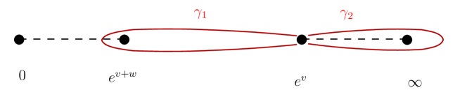
Figure 1. Paths of integration for the twisted periods.

The integration can be performed explicitly by making $\pi(\gamma_{1})$ and $\pi(\gamma_{2})$ tend to the segments $[\mathrm{e}^{v+w},\mathrm{e}^{v}]$ and $[\mathrm{e}^{v},\infty]$. Indeed it is easy to see that

$$\int_{C_{\epsilon}^{\exp(v+w)}}\mathrm{e}^{z\widehat{\lambda}(p)}\frac{\mathrm{d}p}{p}\,\to\ 0\ ,\ \int_{C_{\epsilon}^{\exp(v)}}\mathrm{e}^{z\widehat{\lambda}(p)}\frac{\mathrm{d}p}{p}\,\to\,0\ ,\ \int_{C_{\epsilon}^{\infty}}\mathrm{e}^{z\widehat{\lambda}(p)}\frac{\mathrm{d}p}{p}\,\to\,0$$ (83)

as $\epsilon\to 0$, where $C_{\epsilon}^{a}$ is the (non-closed) lift of a circle of radius $\epsilon$ around $p=a$ and $-1<z<0$.

Moreover, using Euler’s integral representation for the hypergeometric function

$$\phantom{.}_{2}F_{1}(a,b,c,z)=\frac{\Gamma(c)}{\Gamma(b)\Gamma(c-b)}\,\int_{0}^{1}x^{b-1}(1-x)^{c-b-1}(1-zx)^{-a}\mathrm{d}x,$$ (84)

(for $\mathfrak{Re}(c)>\mathfrak{Re}(b)>0$) we can express the remaining line integrals as

$$\begin{split}\mathfrak{p}_{1}(z)=&\frac{1}{2\pi\mathrm{i}}\left(\int_{[\mathrm{e}^{v+w},\mathrm{e}^{v}]}^{+}+\int_{[\mathrm{e}^{v},\mathrm{e}^{v+w}]}^{-}\right)\lambda^{z}(p)\frac{\mathrm{d}p}{p}=\frac{1}{2\pi\mathrm{i}}(1-\mathrm{e}^{2\pi\mathrm{i}z})\,\int_{\mathrm{e}^{v+w}}^{\mathrm{e}^{v}}\,\lambda^{z}(p)\frac{\mathrm{d}p}{p}=\\ &=-z\mathrm{e}^{2\pi\mathrm{i}z}\mathrm{e}^{zv}(1-\mathrm{e}^{w})\phantom{.}_{2}F_{1}(1-z,1+z,2,1-\mathrm{e}^{w})\end{split}$$ (85)

where we used $\Gamma(1+z)\Gamma(1-z)=\frac{\pi z}{\sin(\pi z)}$ and we applied the change of variables $p=\mathrm{e}^{v}(1-(1-\mathrm{e}^{w})x)$ in (84).

Similarly,

$$\begin{split}\mathfrak{p}_{2}(z)=&\frac{1}{2\pi\mathrm{i}}\left(\int_{[\mathrm{e}^{v},\infty]}^{+}+\int_{[\infty,\mathrm{e}^{v}]}^{-}\right)\lambda^{z}(p)\frac{\mathrm{d}p}{p}=\frac{1}{2\pi\mathrm{i}}(1-\mathrm{e}^{2\pi\mathrm{i}z})\,\int_{\exp(v)}^{\infty}\,\lambda^{z}(p)\frac{\mathrm{d}p}{p}=\\ &=\mathrm{e}^{\pi\mathrm{i}z}\mathrm{e}^{zv}\phantom{.}_{2}F_{1}(z,-z,1,\mathrm{e}^{w})\end{split}$$ (86)

where, this time, $x=p$ in (84).

Remark 3.6.

It is worthwhile to stress what happens when we specialize to the suspension by setting $z=1/2$, that is, when we compute the odd periods of $\mathcal{M}_{AL}$. In this case, the universal cover $X$ reduces to an elliptic curve, and we obtain

$$\mathfrak{p}_{1}\left(\frac{1}{2}\right) = \frac{2e^{v/2}\left(E\left(1-e^{w}\right)-K\left(1-e^{w}\right)\right)}{\pi\left(e^{w}-1\right)}$$ (87)

$$\mathfrak{p}_{2}\left(\frac{1}{2}\right) = -\frac{2ie^{v/2}E(e^{w})}{\pi}$$ (88)

where $K(x)$ and $E(x)$ denote the complete elliptic integrals of the first and second kind respectively. Remarkably, upon identifying $u:=\mathrm{e}^{v}(1-\mathrm{e}^{w/2})$, $\Lambda^{4}:=\mathrm{e}^{v+w}$, (87)-(88) yield respectively the derivative of the effective prepotential and the quantum Coulomb branch parameter of $\mathcal{N}=2$ $SU(2)$ super Yang–Mills theory in four dimensions [Seiberg:1994rs], in a vacuum parameterized by a classical value $u=\left\langle\operatorname{Tr}\phi^{2}\right\rangle$ for the adjoint scalar and with RG invariant scale $\Lambda$.

The twisted periods (85)-(86) give a basis of solutions for the deformed flatness conditions associated with the prepotential (80). We thus recover from the LG perspective the observation of [Brini:2010ap] that the quantum differential equation for $\mathcal{O}_{\mathbb{P}^{1}}(-1)_{[-\nu]}\oplus\mathcal{O}_{\mathbb{P}^{1}}(-1)_{[\nu]}$ factorizes in the product of an exponential ODE satisfied by $v$ (as required by the string -axiom) and a Gauss ODE in the variable $w$. The choice of cycles in (85)-(86) however turns out to be non-canonical from the point of view of Gromov–Witten theory; in particular, they are related by an affine transformation to the topological deformed flat coordinates $\mathfrak{p}_{\alpha}^{\mathrm{top}}(z)=\sum_{p=0}^{\infty}\mathfrak{p}_{\alpha,p}^{\mathrm{top}}$ for the resolved conifold, i.e. those deformed flat coordinates for the associated non-homogeneous Frobenius manifold such that

$$\mathfrak{p}_{\alpha,p}^{\mathrm{top}}:=\partial_{t^{\alpha,p}}\mathcal{F}_{0},$$ (89)

where now $\mathcal{F}_{0}$ is the restriction to genus zero and to primary fields of the Gromov–Witten potential (2) of $\mathcal{O}_{\mathbb{P}^{1}}(-1)_{[\nu]}\oplus\mathcal{O}_{\mathbb{P}^{1}}(-1)_{[-\nu]}$. Explicitly, it was found in [Brini:2010ap] that

$$\begin{split}\mathfrak{p}^{\rm top}_{1}(z)=&\left(-\frac{1}{z}+\pi\cot(\pi z)-2\gamma\right)\phantom{.}_{2}F_{1}(-z,z,1,\mathrm{e}^{w})\mathrm{e}^{vz}\\ &-\frac{\pi z}{\sin{\pi z}}\phantom{.}_{2}F_{1}(z+1,-z+1,2,1-\mathrm{e}^{w})(1-\mathrm{e}^{w})\mathrm{e}^{vz}\\ \mathfrak{p}^{\rm top}_{2}(z)=&\frac{\phantom{.}{}_{2}F_{1}(-z,z,1,\mathrm{e}^{w})\mathrm{e}^{vz}-1}{z}\end{split}$$ (90)

where $\gamma$ is the Euler-Mascheroni constant. By comparing with our formulas above for the oscillating integrals, we find

$$\left(\begin{array}[]{c}\mathfrak{p}^{\mathrm{top}}_{1}(z)\\ \mathfrak{p}_{2}^{\mathrm{top}}(z)\end{array}\right)\,=\,\left(\begin{array}[]{cc}0&\frac{\mathrm{e}^{-\mathrm{i}\pi z}}{z}\\ \frac{\mathrm{e}^{-2\mathrm{i}\pi z}(1+2z\gamma-\pi z\cot(\pi z))}{z^{2}}&-\pi\mathrm{e}^{-\mathrm{i}\pi z}z\csc(\pi z)\end{array}\right)\left(\begin{array}[]{c}\mathfrak{p}_{1}(z)\\ \mathfrak{p}_{2}(z)\end{array}\right)-\left(\begin{array}[]{c}\frac{1}{z}\\ 0\end{array}\right).$$

4. Outlook

We list here some possible developments of this work. First of all, the bi-Hamiltonian structure we constructed deserves further investigation: it would be important, on one hand, to elucidate the relation with the bi-Hamiltonian structure of 2D-Toda, and on the other, to find a full dispersive formulation of the pencil. Moreover, the factorization of the Lax matrices that we observe in the Toeplitz reduction points to a generalization of this system to a class of rational reductions of the 2D-Toda hierarchy and, in the dispersionless limit, to corresponding examples of (almost) Frobenius manifolds.

Secondarily, our study of the Frobenius structure (36) suggests that an interesting generalization of the Dubrovin–Zhang theory should find a place in the case of conformal Frobenius manifolds with non-costant unit, and, correspondingly, of bi-Hamiltonian hierarchies with non-exact Poisson pencils. On a more practical note, we remark also that the second half of the Levelt basis for (36) needs further understanding and an explicit construction.

On the dual side, an enticing possibility would be to leverage our construction of a Landau–Ginzburg mirror in order to shed some light on the higher genus theory, and to generalize the picture to more general target spaces. We leave these problems for future investigation.

Appendix A The semi-infinite Toeplitz lattice

The semi-infinite Lax matrices are obtained by restricting the matrix indices in  (8)-(9) to non-negative values. They are indeed simply given by the lower-right blocks in (7):

$$L_{1}=\left(\begin{tabular}[]{lllll}$-x_{1}y_{0}$&$1$&$0$&$0$&\\ $-v_{1}x_{2}y_{0}$&$-x_{2}y_{1}$&$1$&$0$&\\ $-v_{1}v_{2}x_{3}y_{0}$&$-v_{2}x_{3}y_{1}$&$-x_{3}y_{2}$&$1$&\\ $-v_{1}v_{2}v_{3}x_{4}y_{0}$&$-v_{2}v_{3}x_{4}y_{1}$&$-v_{3}x_{4}y_{2}$&$-x_{4}y_{3}$&\\ &&&&$\ddots$\\ \end{tabular}\right),$$

$$L_{2}=\left(\begin{tabular}[]{lllll}$-x_{0}y_{1}$&$-x_{0}y_{2}$&$-x_{0}y_{3}$&$-x_{0}y_{4}$&\\ $1-x_{1}y_{1}$&$-x_{1}y_{2}$&$-x_{1}y_{3}$&$-x_{1}y_{4}$&\\ ~{}~{}$0$&$1-x_{2}y_{2}$&$-x_{2}y_{3}$&$-x_{2}y_{4}$&\\ ~{}~{}$0$&~{}~{}$0$&$1-x_{3}y_{3}$&$-x_{3}y_{4}$&\\ &&&&$\ddots$\\ \end{tabular}\right).$$

The first Lax matrix still factorizes as

$$L_{1}=AB^{-1}$$

with semi-infinite matrices $A$, $B$ still given by (13), while for $L_{2}$ we have

$$L_{2}=BA^{-1}+E$$ (91)

where the matrix $E$, which is zero except for the first row, is given by

$$E_{n,m}=\frac{v_{0}}{y_{0}}\delta_{n,0}y_{m+1},\qquad n,m\geq 0.$$

This is due to the fact that, in the semi-infinite case, the matrix $\Lambda^{-1}$ is the right-inverse of $\Lambda$ but not its left-inverse; indeed, in this case

$$\Lambda^{-1}\Lambda=1-\mathcal{E}$$ (92)

with $\mathcal{E}$ everywhere zero but in the upper-left corner, where it is equal to $1$. In the proof of Proposition 2.2 the left-inverse property of $\Lambda^{-1}$ is used only in the factorization of $L_{2}$; using (92) instead, we easily obtain (91).

In the semi-infinite case, the matrix product $L_{1}L_{2}$ does not involve infinite sums and the problem with associativity mentioned in Remark 2.5 does not arise. We need however to correct $L_{2}$ with the contribution of $E$; we have

Proposition A.1.

In the semi-infinite Toeplitz lattice the Lax matrices satisfy the constraint

$$L_{1}\hat{L}_{2}=1,$$

where

$$\hat{L}_{2}=L_{2}-E=\left(\begin{tabular}[]{lllll}$-\frac{y_{1}}{y_{0}}$&$-\frac{y_{2}}{y_{0}}$&$-\frac{y_{3}}{y_{0}}$&$-\frac{y_{4}}{y_{0}}$&\\ $1-x_{1}y_{1}$&$-x_{1}y_{2}$&$-x_{1}y_{3}$&$-x_{1}y_{4}$&\\ ~{}~{}$0$&$1-x_{2}y_{2}$&$-x_{2}y_{3}$&$-x_{2}y_{4}$&\\ ~{}~{}$0$&~{}~{}$0$&$1-x_{3}y_{3}$&$-x_{3}y_{4}$&\\ &&&&$\ddots$\\ \end{tabular}\right).$$

Note that the associativity problem is still present for the product $\hat{L}_{2}L_{1}$, which is not equal to the identity matrix.

A special role is played by the constraint $x_{0}y_{0}=1$, which is in particular satisfied by the solution of the semi-infinite Toeplitz lattice obtained from the unitary matrix model [MR1794352]. Under such constraint, which is clearly preserved by the hierarchy (cf. equation (16)), the matrix $E$ vanishes, hence $L_{1}L_{2}=1$.

Remark A.2.

Adler - van Moerbeke have shown [MR1794352, MR1993333] that the ratios

$$x_{n}=(-1)^{n}\frac{\tau_{n}^{(1)}}{\tau_{n}^{(0)}},\quad y_{n}=(-1)^{n}\frac{\tau_{n}^{(-1)}}{\tau_{n}^{(0)}},\quad n\geq 1$$

of the tau-functions of the unitary matrix integral defined by

$$\tau_{n}^{(k)}=\int_{U(n)}(\det M)^{k}\mathrm{e}^{\sum_{j=1}^{\infty}\operatorname{Tr}(s^{(1)}_{j}M^{j}-s^{(2)}_{j}\bar{M}^{j})}\ dM$$

satisfy the semi-infinite Toeplitz lattice with $x_{0}(s)=y_{0}(s)=1$ and $x_{n}(0)=y_{n}(0)=0$ for $n>0$. Since $v_{0}=0$, for such solution we have $L_{1}L_{2}=1$.