Re-examining High Abundance SDSS Mass-Metallicity Outliers: High N/O, Evolved Wolf-Rayet Galaxies?

Abstract

We present new MMT spectroscopic observations of four dwarf galaxies representative of a larger sample observed by the Sloan Digital Sky Survey (SDSS) and identified by Peeples et al. (2008) as low-mass, high oxygen abundance outliers from the mass-metallicity relation. Peeples et al. (2008) showed that these four objects (with metallicity estimates of $8.5\leq 12+\log{(\mbox{O/H})}\leq 8.8$) have oxygen abundance offsets of 0.4-0.6 dex from the M_B luminosity-metallicity relation. Our new observations extend the wavelength coverage to include the [O II] $\lambda\lambda$3726,3729 doublet, which adds leverage in oxygen abundance estimates and allows measurements of N/O ratios. All four spectra are low excitation, with relatively high N/O ratios ($\mbox{N/O}\gtrsim 0.10$), each of which tend to bias estimates based on strong emission lines toward high oxygen abundances. These spectra all fall in a regime where the “standard” strong line methods for metallicity determinations are not well calibrated either empirically or by photoionization modeling. By comparing our spectra directly to photoionization models, we estimate oxygen abundances in the range of $7.9\leq 12+\log{\mbox{(O/H)}}\leq 8.4$, consistent with the scatter of the mass-metallicity relation. We discuss the physical nature of these galaxies that leads to their unusual spectra (and previous classification as outliers), finding their low excitation, elevated N/O, and strong Balmer absorption are consistent with the properties expected from galaxies evolving past the “Wolf-Rayet galaxy” phase. We compare our results to the “main” sample of Peeples et al. (2008) and conclude that they are outliers primarily due to enrichment of nitrogen relative to oxygen, and not due to unusually high oxygen abundances for their masses or luminosities.

1 INTRODUCTION

There is a fundamental relationship between the mass of stars in a galaxy and its metallicity evolution (hereafter, the M-Z relation). Empirically, this has been observed as a luminosity-metallicity relationship for low redshift dwarf galaxies (e.g., Lequeux et al., 1979; Skillman et al., 1989; Lee et al., 2006b, and references therein) and spiral galaxies (e.g., McCall et al., 1985; Garnett & Shields, 1987; Zaritsky et al., 1994; Tremonti et al., 2004, and references therein). This robust relationship is observed over a range of 10 magnitudes in galaxy optical luminosity (e.g., Zaritsky et al., 1994; Tremonti et al., 2004; Lee et al., 2006b). In recent years, galaxies at higher redshifts have also shown a mass-metallicity or luminosity-metallicity relationship, and mounting evidence suggests this relationship evolves with time (e.g., Kobulnicky et al., 2003; Kobulnicky & Kewley, 2004; Shapley et al., 2004; Savaglio et al., 2005; Maiolino et al., 2008, and references therein), but see also Mannucci et al. (2010). Thus, this relationship provides both a very strong constraint on theories of galaxy evolution and a tool to better understand galaxies at higher redshifts.

Tremonti et al. (2004, hereafter T04) derived luminosities, metallicities, and masses for $\sim$53,000 low redshift galaxies observed in the Sloan Digital Sky Survey (SDSS; York et al., 2000) and convincingly demonstrated that the basis of the empirically observed luminosity-metallicity relationship is an underlying association between stellar mass and metal abundance. The metallicities were estimated by fitting all observable strong emission lines and deriving a metallicity likelihood distribution for each galaxy based on theoretical model fits calculated using a combination of stellar population synthesis and photoionization models. These models were then used with z-band luminosities to form mass estimates.

The physical driver for the M-Z relationship is still debated. Many studies favor supernova driven winds for the inability of a low-mass galaxy to retain its newly synthesized heavy elements, resulting in a lower effective yield with decreasing mass (e.g., Dekel & Silk, 1986). Other observational and theoretical studies are critical of this theory. For example, Dalcanton (2007) emphasizes the additional importance of star formation efficiency as outflows are an insufficient regulator in the absence of depressed star formation. Thus, a better understanding of the mass-metallicity relationship remains important.

Although the M-Z relationship is well defined, it shows measurable scatter. Since observational error accounts for only half of the metallicity spread in the M-Z relation (Cooper et al., 2008), one or more physical processes may be responsible for the remainder. Suggestions for the scatter include variations in the star formation history (e.g., recent starbursts, Contini et al., 2002), variations in stellar surface mass density (Ellison et al., 2008), and variations in local galaxy density (e.g., Cooper et al., 2008, and references therein). Motivated by the fact that outliers often provide key insights into the nature of physical relationships (e.g., Skillman et al., 1996), Peeples et al. (2008, hereafter P08) and Peeples et al. (2009) identified samples of outlier galaxies from the T04 study.

P08 analyzed a sample of 41 high oxygen abundance, low-luminosity galaxy outliers from the M-Z relation of T04. Their “main” sample is comprised of 24 high abundance (8.95 $\leq$ 12 + log(O/H) $\leq$ 9.27), relatively low-mass (9.1 $\leq$ log$(\mbox{M}_{\star}/\mbox{M}_{\odot})$ $\leq$ 9.9), low-luminosity (sub-L_⋆; $-$19 $\leq$ M_B $\leq$ $-17$) dwarf galaxies. A redshift lower limit of z $>0.024$ was imposed to ensure the inclusion of the [O II] $\lambda\lambda 3726,3729$ emission doublet in the SDSS spectral coverage. The data set was extended to include even lower mass galaxies, creating a second “very low mass” sample, with 7.4 $\leq$ log$(\mbox{M}_{\star}/\mbox{M}_{\odot})$ $\leq$ 9.0, $-$17 $\leq$ M_B $\leq$ $-14$, and 8.68 $\leq$ 12 + log(O/H) $\leq$ 9.12. In order to increase the sample to these lower masses, the redshift limit was dropped. All galaxies in the resulting “very low mass” sample have z $<0.024$, and thus lack an [O II] $\lambda\lambda 3726,3729$ spectral measurement. The typical oxygen abundance offset in the O/H - M_B plane for a galaxy in the “main” sample is $\approx$ 0.4 dex, while the typical offset for the “very low mass” sample is $\approx$ 0.6 dex (with offsets as large as $\approx$ 0.9 dex).

P08 favored isolated or undisturbed systems with relatively low gas mass fractions nearing the end of their star formation activity as an explanation for the unexpectedly high oxygen abundances. Other possible causes for the high abundance outliers were considered and ruled out, such as discrepantly low luminosities for their masses or inaccurate metallicity calculations.

Nebular oxygen abundances derived from the observations of strong emission lines and in the absence of direct measurements of the electron temperature are always subject to systematic effects (e.g., Kennicutt et al., 2003, and references therein). This is particularly true at the higher abundances typically found in spiral galaxies where several calibrations of methods based solely on strong lines result in systematically higher oxygen abundances when compared to oxygen abundances derived from direct measurements of the electron temperature (see, e.g., discussion in Bresolin, 2007, and references therein). Importantly, Yin et al. (2007) and Pérez-Montero & Contini (2009) have pointed out that strong line calibrators that are based on the strength of the [N II] $\lambda\lambda$6548,6584 emission lines are biased in the sense that large values of N/O lead to overestimates of the oxygen abundance. At lower values of oxygen abundance, in general, the strong line methods show better agreement with the oxygen abundances derived from direct temperature measurements, but van Zee et al. (2006b) have shown that there can be significant discrepancies at low values of excitation ($\lambda$5007/$\lambda$3727). Given the uncertainties in strong line oxygen abundance measurements, it is warranted to reinvestigate the conclusions of P08.

The prospect of galaxy outliers from the M-Z relationship, and their consequences for galaxy evolution models, motivated the re-analysis of these objects. In this paper we discuss the previous SDSS and new MMT observations in § 2 and describe the analysis of the latter in § 3. In § 4 we use our new observations of the [O II] $\lambda\lambda 3726,3729$ emission lines to compare the properties of the outliers to the SDSS galaxies. Section 5 is dedicated to looking at several metallicity determinations and the appropriate applications, including the O3N2 method (§ 5.3.1), the N2 indicator (§ 5.3.2), and the R₂₃ index (§ 5.3.3). Our best estimates of the oxygen abundances, the nature of the objects in the “very low mass” sample that gives rise to their discrepant spectra, and an inspection of the nature of the objects in the P08 “main” sample are discussed in § 6.

2 DATA

2.1 Sample

Four of the 17 metal-rich galaxies identified by P08 as “very low mass” ($\log(\mbox{M}_{\star}$/M${}_{\odot})<8.7$) outliers from the M-Z relationship were selected for follow-up observations with the MMT (see Table 1). These targets were chosen both for their significant departures from the mass-metallicity relationship and their availability during a single scheduled observing run. They have suggested high metallicities, as measured by T04, of $8.69\leq 12+\log(\mbox{O/H})\leq 8.86$. For SDSS J022628.28+010937.7, SDSS J024121.80+000329.2, SDSS J082639.19+253553.5, and SDSS J082633.77+252959.2 respectively (hereafter abbreviated as SDSS- plus the first six digits of the Right Ascension), these oxygen abundances lie 0.37, 0.40, 0.55, and 0.55 dex above (and well outside the $\sim$ 0.1 dex scatter of) the luminosity-metallicity relationship histogram medians presented by P08. Like all of the objects in the P08 parent sample, these four galaxies are fairly isolated, low-redshift ($0.0051<z<0.0227$) dwarfs ($-17<\mbox{M}_{B}<-15$), with no obvious companions and somewhat depressed star formation rates (P08).

Table 1: Present Sub-Sample of Low-Luminosity Outliers from Peeples et al. 2008

Object	SDSS Spectra	RA	DEC	MB	log M⋆	Redshift	g-r
SDSS J022628.28+010937.7	spSpec-51869-0406-561.fits	36.6179	1.16053	-16.86	7.92	0.0051	0.51
SDSS J024121.80+000329.2	spSpec-52177-0707-355.fits	40.3408	0.05813	-16.56	8.70	0.0227	0.46
SDSS J082639.19+253553.5	spSpec-52945-1586-164.fits	126.6633	25.59821	-15.87	8.59	0.0078	0.71
SDSS J082633.77+252959.2	spSpec-52945-1586-161.fits	126.6407	25.49979	-15.23	8.07	0.0072	0.55

Note. — Publicly available SDSS spectra can be found at SDSS.org. The RA, DEC, M_B, log M$\star$, and redshift values are taken from P08 (see their Table 1 for more details). The SDSS DR 7 provided g-r colors.

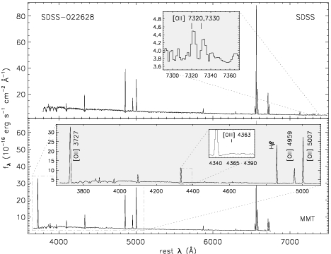
Figure 1: Spectra of SDSS J022628.28+010937.7. The two panels compare the optical H II region spectra from the SDSS and the MMT. Note that the SDSS spectral bandpass does not contain [OII] $\lambda$3727, but does encompass measurable [O II] $\lambda\lambda$7320,7330, as shown in the upper inset box. The bottom inset box is an enlarged view of the MMT spectrum to emphasize the dominance of [O II] over [O III]. This scale also reveals the significant [N II] $\lambda\lambda$6548,6584 strength and the lack of a [O III] $\lambda$4363 detection.

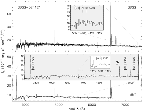
Figure 2: Same as Figure 1, but the spectra are of SDSS J024121.80+000329.2. The SDSS spectrum is too noisy to detect the [O II] $\lambda\lambda$7320,7330 doublet, but displays the strong nitrogen lines. Again, note the strength of the [O II] $\lambda$3727 emission relative to the [O III] emission in the MMT spectrum.

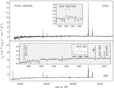
Figure 3: Same as Figure 1, but the spectra are of SDSS J082639.19+253553.5. The SDSS spectrum falls short of capturing the [O II] $\lambda$3727 line and lacks the high signal to noise needed to detect the red [O II] lines. Below, in the MMT spectrum, the [O II] $\lambda$3727 line strength exceeds that of the [O III] $\lambda\lambda$4959,5007 doublet. Also notice the strong [N II] $\lambda\lambda$6548,6584 lines.

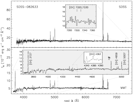
Figure 4: Same as Figure 1, but the spectra are of SDSS J082633.77+252959.2. The MMT spectrum for this object has the most prominent [O II] $\lambda$3727 line relative to the [O III] doublet and, again, strong [N II] lines. Note that while [O III] $\lambda$4363 appears to be measurable, its flux is less than the 3 $\sigma$ uncertainty, and so was not used.

2.2 SDSS Spectra

The measurements made by T04 and used by P08 were derived from the publicly available SDSS Data Release 4 (Adelman-McCarthy et al., 2006) data files referenced in Table 1. We used the SDSS pipeline reduced spectra (rather than performing our own 1-D extraction and reductions) to minimize differences between analyses. For a thorough description of the data reduction refer to Adelman-McCarthy et al. (2006). While the median signal-to-noise (S$/$N) values for the SDSS spectra (12–47) meet the S/N (per pixel) $>8$ requirement for reliable metallicity estimates (Kobulnicky et al., 1999), the wavelength coverage (3800–9200 Å) excludes the [O II] $\lambda$3727 emission line from their spectra. Although the red [O II] $\lambda\lambda$7320,7330 lines are included in the wavelength range, they are only detected in the spectrum of SDSS-022628. In Figures 1-4, we have indicated the locations of the [O II] $\lambda$3727 and [O II] $\lambda\lambda$7320,7330 emission lines.

In § 4 and later in the paper, we compare galaxies from P08 to samples from the SDSS. In these comparisons, we use values of nebular emission line strengths, stellar absorption line strengths, star formation rates, and stellar masses based on SDSS spectra and photometry from the MPA-JHU data catalogue. Stellar masses were determined based on fits to photometry following the work of Kauffmann et al. (2003), and star formation rates (SFR) were based on Brinchmann et al. (2004) and Salim et al. (2007). Objects with [O II], [O III], H$\beta$, [N II], and H$\alpha$ line strengths less than 5 $\sigma$ were filtered out in order to increase the quality of this data set.

2.3 MMT Spectra

2.3.1 Observations

New MMT observations were acquired in order to obtain improved S$/$N spectra and extended blue wavelength coverage including the [O II] $\lambda$3727 line. The MMT data were taken with the Blue Channel spectrograph (Schmidt et al., 1989) on the UT date of 2008 November 1-2. Sky conditions were optimal with no cloud cover and sub-arcsecond seeing. A 500 line grating, $1\arcsec$ slit, and UV-36 blocking filter were used, yielding an approximate dispersion of 1.2 Å per pixel, a full width at half maximum resolution of $\lesssim 3$ Å, and a wavelength coverage of 3690–6790 Å. Bias frames, flat-field lamp images, and sky flats were taken each night. The latter were primarily necessary due to significant differences between the chip illumination patterns of the sky and the MMT Top Box that houses the Blue Channel incandescent flat-field lamp. Multiple standard stars from Oke (1990) with spectral energy distributions peaking in the blue and containing minimal absorption were observed throughout the night using a 5$\arcsec$ slit over a range of airmasses.

All four galaxies had strong central brightness peaks which were centered on the $1\arcsec\times 180\arcsec$ slit. Three 900 second exposures (600 seconds for SDSS-086239) were made at a fixed position angle which approximated the parallactic angle at half the total integration time. This, in addition to observing the galaxies at an airmass below 1.5, served to minimize the wavelength-dependent light loss due to differential refraction (Filippenko, 1982). A single slit position for each target was sufficient to characterize the global oxygen abundance, as metallicity gradients are small in low-mass galaxies (e.g., Skillman et al., 1989; Kobulnicky & Skillman, 1996, 1997; Lee et al., 2006a). Finally, combined helium, argon, and neon arc lamps were observed at each pointing for accurate wavelength calibration.

2.3.2 Data Reduction

The MMT observations were processed using ISPEC2D (Moustakas & Kennicutt, 2006), a long-slit spectroscopy data reduction package written in IDL. A master bias frame was created from $\gtrsim 20$ zero second exposures by discarding the highest and lowest value at each pixel and taking the median. Master sky and dome flats were similarly constructed after normalizing the counts in the individual images. Those calibration files were then used to bias-subtract, flat-field, and illumination-correct the raw data frames. Dark current was measured to be an insignificant $\sim 1$ e^- per pixel per hour and was not corrected for.

Misalignment between the trace of the light in the dispersion direction and the orientation of the CCD detector was rectified via the mean trace of the standard stars for each night, providing alignment to within a pixel across the detector. A two-dimensional sky subtraction was performed using individually selected sky apertures, followed by a wavelength calibration applied from the HeArNe comparison lamps taken at the same telescope pointing. Airmass dependent atmospheric extinction and reddening were corrected for using the standard Kitt Peak extinction curve (Crawford & Barnes, 1970).

For each galaxy, the three sub-exposures were combined, eliminating cosmic rays in the process. The resulting images were then flux-calibrated using the sensitivity curve derived from the standard star observations taken throughout a given night. Finally, the trace fit to the strongest continuum source in the slit was used to extract the galaxy light within 15-30$\arcsec$ apertures that encompassed $\gtrsim$ 99% of the spatially smooth and centrally peaked emission. Figures 1-4 show the resulting one-dimensional spectra (with median S/N values $>$ 30) in comparison to the SDSS spectra. Inset windows with a narrower spectral range emphasize the blue emission lines and the dominance of [O II] over [O III] in all four galaxies.

3 ANALYSIS

3.1 Emission Line Measurements

Emission line strengths were measured for both the MMT and SDSS spectra using standard methods available within IRAF. In particular, the SPLOT routine was used to analyze the extracted one-dimensional spectra and fit Gaussian profiles to emission lines to determine their integrated fluxes. The H$\alpha$ and the adjacent [N II] lines were fitted simultaneously for an accurate deblending.

Special attention was paid to the Balmer lines, which are located in troughs of significant underlying stellar absorption. Although the equivalent widths of the H$\alpha$ emission lines were large enough that the underlying absorption was not a concern, this was not the case for H$\beta$ and the bluer Balmer lines. We experimented with several different methods to correct the measurement of the H$\beta$ emission flux for the effects of underlying absorption. At one extreme, maximizing the H$\beta$ line intensity (by overestimating the underlying absorption) leads to a minimum H$\alpha$/H$\beta$ value and a minimum estimate of the reddening. Because the underlying absorption is much broader than the emission and these features are both well resolved and relatively high signal-to-noise, the subtraction of the underlying absorption represents only a small contribution to the uncertainty in the reddening corrections (see Table 2).

For our final analysis of the Balmer emission lines, we used the PAN analysis package to simultaneously fit the continuum, the Gaussian emission peak, and a broad, negative Lorentzian absorption feature. PAN uses a least-squares fit to minimize $\chi^{2}$ and estimates the uncertainty using a “bootstrap” Monte Carlo error analysis, providing a reliable measurement of the flux and associated uncertainty of the Balmer emission line. Figure 5 exhibits both the individual component and total fits determined by PAN, with minimal residuals validating the goodness of fit to our spectra. The emission line fluxes are reported relative to H$\beta$ in Table 2, and represent the multiple component fits for the H$\beta$ and H$\gamma$ emission lines and the single or deblended Gaussian profile fits from SPLOT for the rest of the emission lines.

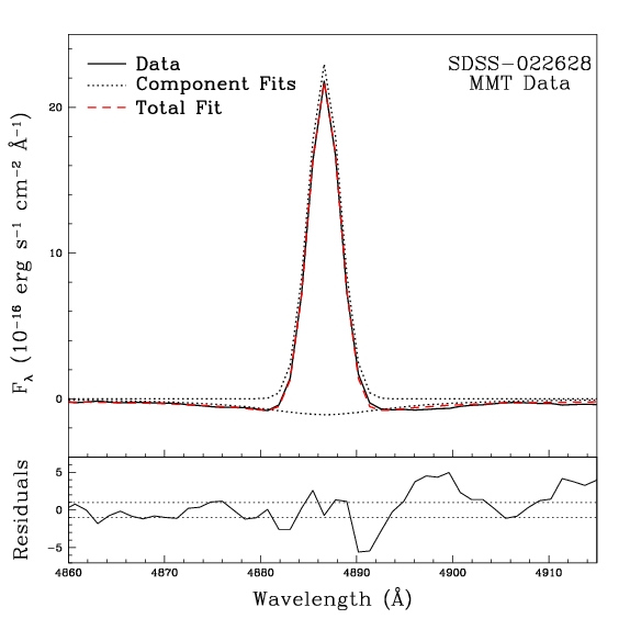
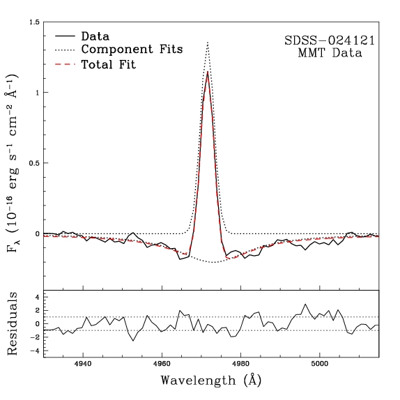
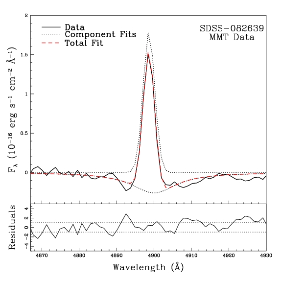
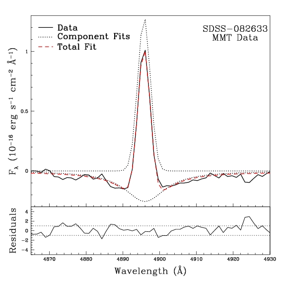
Figure 5: H$\beta$ region of the MMT spectra, as measured in PAN. The dotted gray lines correspond to the Lorentzian absorption and Gaussian emission component fits. The red dashed line displays the best overall fit to the original data (solid black line). The residual difference between the fit and data is shown in the bottom panel, with very little divergence near the emission peak, confirming a successful fit. The ensuing H$\beta$ emission flux, accounting for Balmer absorption, can be found in Table 2.

The errors of the flux measurements were approximated using

$$\sigma\approx 2\sqrt{N}\ rms,$$ (1)

where N is the number of pixels spanning the Gaussian profile fit to the narrow emission lines (typically 11). The rms noise in the continuum was taken to be the average of the rms on each side of an emission line. This error approximation is valid for weak lines whose uncertainty is dominated by error from the continuum subtraction. For cases where the flux measurements were much stronger than the rms noise of the continuum, the error is dominated by flux calibration and de-reddening uncertainty. This is true for several lines in both the SDSS and MMT spectra of SDSS-022628, and for all the H$\alpha$ lines (where a minimum uncertainty of 2% was assumed). Flux line strengths relative to H$\beta$ and corresponding errors are listed in Table 2. As we were not able to detect [O III] $\lambda$4363 and He II $\lambda$4686 at the level of more than 3 $\sigma$ in any of the spectra, a flux upper limit was estimated using Equation 1. We calculated upper limits on the electron temperatures based on these $\lambda$4363 fluxes, but none provided significant constraints for abundance calculations. In some cases, the H$\alpha$/H$\beta$ ratios for the SDSS and MMT spectra are significantly different. Using the MMT data for our reference ratio, the average percentage difference between the SDSS and MMT H$\alpha$/H$\beta$ ratio is 15%, whereas the average [O III] $\lambda$5007/H$\beta$ percentage difference is 16%. Since the [O III]/H$\beta$ ratio is less sensitive to flux calibrations, these differences between the two data sets are likely due to using long-slit (MMT spectra) versus circular fiber apertures (SDSS spectra).

3.2 Reddening Corrections

The wide range of observed wavelengths require fluxes to be corrected for extinction and reddening. Since the relative intensities of the Balmer lines are nearly independent of both density and temperature, they can be used to solve for the reddening. Assuming standard H II region characteristics (T${}_{e}=1.25\times 10^{4}$ K and n${}_{e}=10^{2}$ cm^-3), both the MMT and SDSS spectra were de-reddened using a Balmer decrement of 2.82 (Hummer & Storey, 1987) and the Cardelli et al. (1989) reddening law (with A${}_{V}=3.1\ E(B-V)$). The extinction, $A_{1}(\lambda)$, from the Cardelli et al. (1989) law was calculated using the York Extinction Solver (McCall, 2004). With these values we then derived the reddening value, $E(B-V)$, using

$$\log{\frac{I(H\alpha)}{I(H\beta)}\ }=\log{\frac{F(H\alpha)}{F(H\beta)}\ }+0.4\ E(B-V)\ [A_{1}(H\alpha)-A_{1}(H\beta)],$$ (2)

where F(H$\alpha$)/F(H$\beta$) is the observed flux ratio and I(H$\alpha$)/I(H$\beta$) is the de-reddened line intensity ratio using case B from Hummer & Storey (1987). Following Lee & Skillman (2004) the reddening value can be converted to the logarithmic extinction at $H\beta$ as

$$c(H\beta)=1.43\ E(B-V).$$ (3)

Original and de-reddened flux values for both the MMT and SDSS data are given in Table 2, where errors were propagated from those associated with the individual line measurements. All of the H$\alpha$/H$\beta$ ratios are larger than 2.82, indicative of significant extinction and reddening due to dust. Since the Galactic latitudes for the four galaxies are all large (ranging from $31\arcdeg$ to $54\arcdeg$), little foreground extinction from Galactic dust is expected, and, indeed, the calculated values of $E(B-V)$ (see Table 2) are substantially greater than the foreground extinction determined by Schlegel et al. (1998). Our reddening corrections can be checked by comparing the corrected H$\gamma$/H$\beta$ ratios with their theoretical values. As seen in Table 2, this ratio is consistent with the theoretical case B recombination ratio of 0.47 (Hummer & Storey, 1987) in all four cases. This result implies accurate reddening corrections were made, which strengthens the argument for significant intrinsic extinction.

Table 2: Normalized and Reddening Corrected Emission Line Intensity Ratios for the Observed Sample

	SDSS-022628			SDSS-024121			SDSS-082639			SDSS-082633
MMT Data	F($\lambda$)/F(H$\beta$)	I($\lambda$)/I(H$\beta$)		F($\lambda$)/F(H$\beta$)	I($\lambda$)/I(H$\beta$)		F($\lambda$)/F(H$\beta$)	I($\lambda$)/I(H$\beta$)		F($\lambda$)/F(H$\beta$)	I($\lambda$)/I(H$\beta$)
[O II] $\lambda$3727	2.12$\pm$0.06	2.47$\pm$0.09		2.62$\pm$0.13	4.13$\pm$0.22		1.89$\pm$0.12	3.67$\pm$0.25		3.50$\pm$0.17	3.90$\pm$0.22
H$\gamma$ $\lambda$4340	0.40$\pm$0.01	0.43$\pm$0.01		0.33$\pm$0.04	0.41$\pm$0.05		0.37$\pm$0.06	0.49$\pm$0.08		0.34$\pm$0.05	0.38$\pm$0.05
[O III] $\lambda$4363	$<$ 0.02 (3 $\sigma$)	$<$ 0.02 (3 $\sigma$)		$<$ 0.12 (3 $\sigma$)	$<$ 0.14 (3 $\sigma$)		$<$ 0.15 (3 $\sigma$)	$<$ 0.19 (3 $\sigma$)		$<$ 0.16 (3 $\sigma$)	$<$ 0.17 (3 $\sigma$)
He II $\lambda$4686	$<$ 0.01 (3 $\sigma$)	$<$ 0.01 (3 $\sigma$)		$<$ 0.10 (3 $\sigma$)	$<$ 0.10 (3 $\sigma$)		$<$ 0.15 (3 $\sigma$)	$<$ 0.16 (3 $\sigma$)		$<$ 0.10 (3 $\sigma$)	$<$ 0.10 (3 $\sigma$)
H$\beta$ $\lambda$4861	1.00$\pm$0.03	1.00$\pm$0.03		1.00$\pm$0.04	1.00$\pm$0.04		1.00$\pm$0.03	1.00$\pm$0.03		1.00$\pm$0.06	1.00$\pm$0.06
[O III] $\lambda$4959	0.39$\pm$0.01	0.39$\pm$0.01		0.28$\pm$0.04	0.27$\pm$0.03		0.18$\pm$0.05	0.17$\pm$0.05		0.32$\pm$0.08	0.31$\pm$0.08
[O III] $\lambda$5007	1.18$\pm$0.03	1.16$\pm$0.03		0.70$\pm$0.04	0.67$\pm$0.04		0.54$\pm$0.05	0.50$\pm$0.05		0.95$\pm$0.09	0.93$\pm$0.09
He I $\lambda$5876	0.12$\pm$0.02	0.11$\pm$0.02		0.15$\pm$0.02	0.11$\pm$0.02		0.23$\pm$0.04	0.15$\pm$0.03		0.13$\pm$0.02	0.13$\pm$0.02
[N II] $\lambda$6548	0.20$\pm$0.01	0.17$\pm$0.01		0.35$\pm$0.04	0.23$\pm$0.02		0.42$\pm$0.05	0.23$\pm$0.03		0.19$\pm$0.05	0.15$\pm$0.04
H$\alpha$ $\lambda$6563	3.24$\pm$0.10	2.79$\pm$0.08		4.30$\pm$0.15	2.79$\pm$0.10		5.19$\pm$0.15	2.79$\pm$0.10		3.50$\pm$0.16	2.79$\pm$0.13
[N II] $\lambda$6584	0.63$\pm$0.02	0.55$\pm$0.02		1.02$\pm$0.05	0.67$\pm$0.03		1.38$\pm$0.06	0.74$\pm$0.04		0.71$\pm$0.06	0.57$\pm$0.04
H$\beta$ Flux	956$\pm$19			57.7$\pm$1.7			70.3$\pm$1.4			55.4$\pm$2.3
H$\beta$ EW	-23.6$\pm$0.7			-6.1$\pm$0.8			-4.9$\pm$0.9			-5.1$\pm$0.9
H$\beta$ Abs EW	5.7$\pm$0.2			8.1$\pm$0.5			6.9$\pm$0.3			7.0$\pm$0.4
H$\alpha$ EW	-87.2$\pm$1.8			-34.5$\pm$2.5			-25.7$\pm$1.4			-24.9$\pm$1.8
E(B-V)	0.14$\pm$0.01			0.42$\pm$0.02			0.62$\pm$0.03			0.22$\pm$0.01
C(H$\beta$)	0.20$\pm$0.01			0.61$\pm$0.02			0.88$\pm$0.03			0.31$\pm$0.01
	SDSS-022628			SDSS-024121			SDSS-082639			SDSS-082633
SDSS Data	F($\lambda$)/F(H$\beta$)	I($\lambda$)/I(H$\beta$)		F($\lambda$)/F(H$\beta$)	I($\lambda$)/I(H$\beta$)		F($\lambda$)/F(H$\beta$)	I($\lambda$)/I(H$\beta$)		F($\lambda$)/F(H$\beta$)	I($\lambda$)/I(H$\beta$)
H$\beta$ $\lambda$4861	1.00$\pm$0.03	1.00$\pm$0.03		1.00$\pm$0.11	1.00$\pm$0.11		1.00$\pm$0.09	1.00$\pm$0.09		1.00$\pm$0.09	1.00$\pm$0.09
[O III] $\lambda$4959	0.39$\pm$0.02	0.38$\pm$0.02		0.18$\pm$0.07	0.17$\pm$0.07		$\cdots$	$\cdots$		0.37$\pm$0.07	0.36$\pm$0.07
[O III] $\lambda$5007	0.92$\pm$0.03	0.88$\pm$0.03		0.61$\pm$0.09	0.59$\pm$0.08		0.42$\pm$0.08	0.39$\pm$0.07		1.00$\pm$0.09	0.96$\pm$0.09
[N II] $\lambda$6548	0.28$\pm$0.01	0.19$\pm$0.01		0.30$\pm$0.04	0.23$\pm$0.03		0.42$\pm$0.05	0.22$\pm$0.02		0.22$\pm$0.05	0.15$\pm$0.03
H$\alpha$ $\lambda$6563	4.09$\pm$0.13	2.79$\pm$0.09		3.71$\pm$0.29	2.79$\pm$0.22		5.34$\pm$0.34	2.79$\pm$0.18		4.02$\pm$0.28	2.79$\pm$0.19
[N II] $\lambda$6584	0.87$\pm$0.03	0.60$\pm$0.02		0.95$\pm$0.08	0.72$\pm$0.06		1.46$\pm$0.10	0.77$\pm$0.05		0.74$\pm$0.07	0.52$\pm$0.05
[O II] $\lambda$7320	0.03$\pm$0.01	0.02$\pm$0.01		$\cdots$	$\cdots$		$\cdots$	$\cdots$		$\cdots$	$\cdots$
[O II] $\lambda$7330	0.02$\pm$0.01	0.01$\pm$0.01		$\cdots$	$\cdots$		$\cdots$	$\cdots$		$\cdots$	$\cdots$
H$\beta$ Flux	979$\pm$24			87.2$\pm$6.6			114.7$\pm$7.2			88.0$\pm$5.8
H$\beta$ EW	-23.5$\pm$1.2			-5.4$\pm$2.1			-5.5$\pm$1.2			-5.9$\pm$1.8
H$\beta$ Abs EW	9.8$\pm$0.4			7.5$\pm$0.6			9.5$\pm$0.4			7.2$\pm$0.6
H$\alpha$ EW	-89.5$\pm$2.9			-30.7$\pm$2.3			-27.9$\pm$0.9			-28.8$\pm$2.1
E(B-V)	0.37$\pm$0.02			0.28$\pm$0.01			0.64$\pm$0.03			0.36$\pm$0.02
Galactic Lat.	-53.626			-52.102			31.400			31.351
Galactic E(B-V)	0.031			0.029			0.080			0.070

Note. — The spectra were de-reddened assuming Hummer & Storey (1987) case B for T${}_{e}=1.25\times 10^{4}$ K and n${}_{e}=$ 100 cm^-3 and the Cardelli et al. (1989) reddening law with $R_{\mbox{v}}=3.1$. For each galaxy, the measured flux ratio is given by F($\lambda$)/F(H$\beta$), and the dereddened flux ratio by I($\lambda$)/I(H$\beta$). The Galactic $E(B-V)$ is taken from Schlegel et al. (1998). The equivalent widths measure the H$\beta$ and H$\alpha$ Balmer emission lines using SPLOT, and the broad H$\beta$ absorption features using PAN. EWs are given in units of Å.

4 COMPARISON OF SAMPLE GALAXIES TO THE SDSS

Our new observations allow us to examine these Peeples et al. (2008) galaxies against larger samples drawn from the MPA-JHU SDSS database. Since the “very low mass” sample lacked [O II] measurements, we are particularly interested in how the strengths of these emission lines compare. Figure 6 illustrates properties of the four observed galaxies with respect to star-forming galaxies in the SDSS that fall in the “very low mass” sample range of $7\leq$ log(M_⋆/M${}_{\odot})\leq 9$. We have further restricted the SDSS comparison sample to those objects with s/n $\geq$ 5 in the relevant lines.

The top panel in Figure 6 shows a comparison of the excitation, measured by the [O II]/[O III] ratio. The two more massive galaxies are clearly discrepantly strong in [O II] emission; these are very low excitation galaxies. With decreasing mass, the SDSS comparison sample becomes relatively sparse, but the two lower mass galaxies have comparatively low excitation.

The second panel shows a comparison of the [N II]/[O II] ratio, primarily a function of the N/O abundance. Again, for the two more massive galaxies, there is a clear offset from the locus defined by the SDSS galaxies. While the [N II]/[O II] ratios are of comparable strength in the two lower mass galaxies, the trend in the SDSS sample is less clear. Extrapolating from the higher mass galaxies, the lower mass galaxies would be clearly discrepant, but they lie in the middle of a very sparse scatter in the diagram. Quantitatively, in a comparison with a least-squares fit to the SDSS compilation, the values of log(N/O) for our four observed galaxies are $0.2-0.4$ dex higher than is typical for objects in the same stellar mass range.

The lower two panels compare the equivalent widths of the underlying stellar absorption and the star formation rates derived from H$\alpha$. The four objects presented in this paper have H$\beta$ absorption equivalent widths on the high end of the SDSS distribution and star formation rates on the low side of the distribution.

In sum, the four galaxies which we have observed are outliers in a number of properties. Given that oxygen abundances derived from strong emission lines are subject to a number of systematic uncertainties, it is clearly warranted to revisit their status as oxygen abundance outliers.

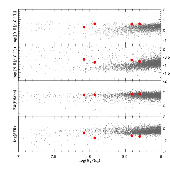
Figure 6: Properties of low-mass star-forming galaxies in the SDSS (gray dots) plotted against stellar mass. The four objects presented in this paper are shown as red dots in comparison. Interestingly, the [N II]/[O II] ratios are well above average for the mass range, and the [O II]/[O III] ratios show that these objects have significantly lower excitation than is typical. Additionally, their star formation rates are relatively low and their H$\beta$ absorption equivalent widths are on the high end of the SDSS range.

5 OXYGEN ABUNDANCE DETERMINATIONS

Relative to the SDSS spectra, our MMT spectra have the advantages of higher signal to noise and the inclusion of the blue [O II] $\lambda$3727 line. Kniazev et al. (2003) showed from SDSS spectra that O⁺/H⁺ ionic abundances can be determined reasonably well by observing the red [O II] $\lambda\lambda$7320,7330 lines (as a substitute for [O II] $\lambda$3727); however, because they are auroral lines, their strong sensitivity to temperature can result in relatively high abundance uncertainties. In all four MMT spectra (Figures 1-4) the preferred [O II] $\lambda$3727 emission line strengths are noticeably stronger than the [O III] $\lambda$5007 lines, underscoring the importance of accurately accounting for the contribution from the lower ionization state in determining oxygen abundances.

Accurate “direct” oxygen abundance determinations from H II regions require a measurement of the electron temperature (typically via observation of the temperature sensitive [O III] $\lambda$4363 auroral line). However, as metallicity increases, cooling via metal lines becomes more efficient and the electron temperature decreases, making these intrinsically faint lines even more difficult to detect. Since we did not reliably detect [O III] $\lambda$4363 in any of our targets, abundances must be estimated empirically or theoretically using relationships dependent upon relative strong line flux ratios.

Alloin et al. (1979) and Pagel et al. (1979) were the first to provide strong-line calibrations, where oxygen abundance is related to one or more ratios of recombination and collisionally excited lines. Several other methods have since been developed and categorized as semi-empirical, empirical, or theoretical. Semi-empirical calibrations were determined using a combination of electron temperature measurements at low metallicity and photoionization models at high metallicity in correspondence with observational limitations. Empirical calibrations result from observations of H II regions with electron temperature measurements. However, the relatively small number of direct oxygen abundance determinations available are typically biased in the sense that they are based upon high-excitation H II regions only. In contrast, theoretical strong-line calibrations use ab initio photoionization models. One advantage to theoretical models is that they allow a wide range in ionization parameter in addition to input metallicity. However, these models rely on simplified assumptions of nebular properties and so do not yet provide entirely realistic representations of H II regions. Most troubling is that all theoretical strong line abundance determination methods over-predict abundances in the metal-rich (roughly solar metallicity and above) regime when compared to abundances determined from direct temperature measurements.

Here we review the original oxygen abundances as determined by T04 using Bayesian models, the revised strong line oxygen abundances calculated by P08, strong line oxygen abundances from our new MMT spectra (with and without the addition of the blue [O II] emission), and the N/O relative abundance ratios. T04 found this type of comparison is valid for SDSS data by showing that analytic R23-metallicity relations roughly bracket the range of metallicities that they derive, concluding that their M-Z relationship is in line with previous strong-line calibrations. The culmination of these efforts is presented in Figure 7, which allows us to compare all of the oxygen abundance estimates with those expected from the M-Z relationship. Note that Figure 7 is shown for illustrative purposes only, and not to suggest which calibrator is more fundamentally correct.

5.1 The T04 Oxygen Abundances

P08 initially identified outliers from luminosities, gas-phase oxygen abundances, and stellar masses provided by T04. The T04 abundance calculations are based on a Bayesian statistical analysis of the strongest six emission lines using stellar population synthesis models from Bruzual & Charlot (2003) and photoionization models from CLOUDY (Ferland et al., 1998). Note that while the T04 abundances were used to identify the outliers (in a self-consistent manner), P08 derived their own abundances, which are systematically lower than the T04 abundances. Yin et al. (2007, hereafter Y07) compared the oxygen abundances from T04 with oxygen abundances derived from direct temperature measurements (using auroral lines) and found the T04 oxygen abundances to be systematically higher on average. Y07 further showed that the magnitude of this offset correlates well with the N/O abundance ratio, and concluded that the offset is due to the assumption of a single N enrichment trend in the underlying Charlot & Longhetti (2001) modeling.

Kewley & Ellison (2008, hereafter KE08) compared the M-Z relationships derived from ten different strong-line methods and found large systematic discrepancies between empirical and theoretical calibrations. In the KE08 study, T04 metallicities tend to be in the middle of the range when low metallicities are considered (12 + log(O/H) $\approx$ 8.5) and at the high end of the range when the high metallicities are considered (12 + log(O/H) $\approx$ 9.0). KE08 provide relations for converting one metallicity scale to another, but the results of the Y07 analysis imply that a simple conversion is not always sufficient. That is, not only can the absolute abundances provided by the strong-line methods be systematically offset from the true nebular abundances, but, in some cases, the strong-line methods do not even accurately rank the abundances (see Table 3 and Figure 7 for different rankings among the 4 objects presented here).

5.2 The P08 Oxygen Abundances

P08 derived their own oxygen abundances for the outliers identified from the T04 sample. Since there was insufficient information to reproduce the results of the Bayesian statistical analysis of T04, P08 used two of the methods investigated by KE08. They used the [N II]/[O II] ratio as calibrated by KE08 for the “main” sample (where [O II] $\lambda$3727 was observed), and the [O III]/[N II] ratio (the “O3N2” method) as calibrated by Pettini & Pagel (2004) for the remaining galaxies in the “very low mass” sample. P08 did not use the $R_{23}$ diagnostic for their “main” sample because of concerns regarding its calibration at high metallicities (the presumed regime for their samples). P08 found that their oxygen abundances derived from the [N II]/[O II] ratio for the “main” sample agreed well with the T04 oxygen abundances. However, the O3N2 abundances were consistently lower than the T04 abundances by roughly 0.3 dex (in concordance with the offsets determined by KE08). The net effect is that the abundances derived by P08 are lower than those derived by T04. P08 concluded that, regardless of the metallicity calibration used, their sample of 41 galaxies are true high-metallicity, low mass outliers from the mass-metallicity relation. Despite any offsets between the T04 and P08 data sets, both use a strong line calibration based partially on [N II] strength, which make abundance estimates liable to overestimates if the galaxies are nitrogen-enhanced (see § 5.3.2 and § 5.4).

5.3 Strong Line Methods Revisited

We have chosen to re-compute the oxygen abundances for this sample using the MMT spectra with several strong line calibrations: the O3N2 method, the N2 method, the R₂₃ index, and determinations using assumed temperatures. This serves to highlight differences amongst methods, outline the resulting range of possible abundances, and demonstrate that strong line calibrations are not appropriate for the present sample. These measurements are discussed below and compared in Figure 7.

5.3.1 “O3N2” Method

The O3N2 method is one of two empirical calibrations used by P08 for the “main” sample, and the only calibration used for the “very low mass” sample since these objects lacked the necessary [O II] measurements. It was introduced by Pettini & Pagel (2004, hereafter PP04) using empirical fits to strong line ratios from H II regions with “direct” oxygen abundances. Derived for the purpose of measuring metallicities in galaxies at high redshift, lines close in wavelength are used to mitigate the need for flux calibrations and reddening corrections. Direct metallicities were compared to the ratio of ([O III] $\lambda$5007/H$\beta$)/([N II] $\lambda$6584/H$\alpha$) for a sample of 137 H II regions. See the resulting O3N2 relationship of Equation 3 in PP04, where O3N2 = $\log$(([O III] $\lambda 5007/$H$\beta$)/([N II] $\lambda 6584/\mathrm{H}\alpha))$.

P08 favored the O3N2 method with its high sensitivity to oxygen abundance. Indeed, O3N2 is a good calibration in the high-metallicity regime, where [N II] tends to saturate, but the strength of [O III] continues to decrease with increasing metallicity. Note that the choice by PP04 to use only objects with direct metallicities, in an effort to provide a more secure calibration, introduces a bias because low excitation spectra (i.e., relatively low values of $\lambda$5007/$\lambda$3727) are excluded from the calibration. Thus, the unintended consequence of the choice to limit the sample to objects which were perceived to have more accurate abundances has resulted in a biased sample. This biased sample gives the impression of a smaller scatter in the relationship than occurs in nature (cf., Yin et al., 2007).

To confirm consistency with P08, we duplicated the O3N2 measurements for the SDSS spectra and calculated O3N2 from our MMT spectra. The results are listed in Table 3 and closely match the measurements by P08 using the same O3N2 methodology; they are lower than the values found by T04 by 0.2 - 0.3 dex.

Y07 showed a large scatter in the comparison of abundances derived from the O3N2 calibration with oxygen abundances derived from the direct method. They suggest that the scatter could be due to excluding the ionization parameter in the O3N2 calibration. The importance of the ionization parameter strengthens in the low-metallicity regime where O3N2 is much less dependent on metallicity. Additionally, at low Z, N is thought to be a primary element, implying that the N/O ratio is independent of O/H.

Since the calibration of the O3N2 method does not account for possible variations in N/O for a given O/H, inherent biases are possible. Pérez-Montero & Contini (2009, hereafter PMC09) found that a strong correlation exists between metallicity derived from the O3N2 parameter and the N/O ratio, such that when the N/O is enhanced, the O3N2 strong line calibration tends to overestimate the O/H abundances. PMC09 corrected for this dependence by using 12 + log(O/H) versus O3N2 residuals to modify the O3N2 calibration (see Equation 8 in PMC09). Using the N/O calculations from § 5.4 and given in Table 4, we calculated the revised O3N2 abundances and list them in Table 3. This calibration lowers the O3N2 abundances only slightly (by an average of $\sim 0.1$ dex) relative to PP04 O3N2 estimates. In § 5.5 we look at the higher abundances from the O3N2 method relative to relationships predicted by direct and photoionization model abundances.

5.3.2 “N2” Indicator

Denicoló et al. (2002, hereafter D02) proposed the use of the [N II] $\lambda$6584/H$\alpha$ ratio as a sensitive metallicity indicator. This is a promising estimator: like O3N2 it eliminates uncertainties due to reddening and flux calibrations, and functions well for metallicity values below the [N II] saturation level. The original N2 calibration developed by D02 (see Equation 2 in D02), where N2 = $\log$([N II] $\lambda 6584/\mathrm{H}\alpha)$, was based on $\sim$155 H II regions and used a least squares fit with an estimated uncertainty of $\sim$0.2 dex. For our objects, this method produces oxygen abundances (8.61 $\leq$ 12 + log(O/H) $\leq$ 8.70) in agreement with the P08 values.

PP04 re-calibrated this parameter, primarily with electron temperature-based metallicities, characterizing the fit both linearly and with a third-order polynomial. The polynomial fit is given in Equation 2 of PP04, yielding oxygen abundances of 8.45 $\leq$ 12 + log(O/H) $\leq$ 8.56. The results for both calibrations are listed in Table 3.

Note, again, as with the PP04 calibration of the O3N2 method, the exclusive use of calibrators determined with measured electron temperatures underestimates the scatter in the relationship, and biases against low-ionization H II regions. Yin et al. (2007) found similar results in their analysis of the N2 method as found for the O3N2 method. The uncertain roles of the ionization parameter and the relationship between N/O and O/H as a function of metallicity result in appreciable uncertainty and scatter in the N2 method. Expanding on this idea, PMC09 found an expectedly strong dependence of metallicities predicted by N2 on the N/O ratio. PMC09 derived a calibration correcting for this effect (see their Equation 13). Using N/O ratios from § 5.4 and tabulated in Table 4, we present the results of this calibration in Table 3. This method predicts oxygen abundances which are $\sim 0.1$ and $\sim 0.2$ dex smaller on average than those predicted by the PP04 and D02 N2 methods respectively. Shifts to smaller oxygen abundances of this size can account for roughly half of the offset from the L-Z and M-Z relationships.

5.3.3 R₂₃ Index

Pagel et al. (1979) promoted the use of the R₂₃ index, R₂₃ = ([O II] $\lambda 3727$ + [O III] $\lambda\lambda$4959, 5007)/(H$\beta$), as a good estimate of oxygen abundance in the absence of an electron temperature measurement. Because the optical [O II] and [O III] emission lines decrease at both high abundances (due to an increasing role of fine structure line cooling) and low abundances (due to the decrease in the relative number of oxygen atoms), the relationship is bi-valued and, therefore, potentially ambiguous. The turn-around in the relationship occurs at oxygen abundances near 12 + log(O/H) $\approx$ 8.4 where R₂₃ reaches a maximum of $\approx$10. However, the degeneracy between the two branches of solutions can, in most situations, be broken with an additional determinant. Also, since R₂₃ is based on emission lines with significant separation in wavelength, accurate reddening corrections and uncertainties are important. Below, we discuss two R₂₃ calibrations, one constructed from photoionization models, and another empirically based. Since P08 believed the sample to be high-metallicity, they did not consider the R₂₃ diagnostic due to the potential of [O II] + [O III] to saturate and the lack of [O II] measurements in their “very low mass” sample.

McGaugh (1991) created a calibration based on theoretical photoionization models using R₂₃ and the additional O₃₂ index: O₃₂ = ([O III] $\lambda\lambda 4959,5007$)/([O II] $\lambda 3727$). McGaugh developed this model using the photoionization code CLOUDY (Ferland et al., 1998) and zero-age H II region models, accounting for photoionization parameter variations. To discriminate between the two branches, van Zee et al. (1998), followed by others, advised using the ratio of ([N II] $\lambda$6584)/([O II] $\lambda$3727). McGaugh (1994) suggested that [N II]/[O II] is approximately $<$ 0.1 for low abundances and $>$ 0.1 for high abundances, giving a rough distinction between lower and upper branches. Note, however, that McGaugh (1994) also points out (his Figure 3) that there is a dependence on the N/O ratio on the behavior of this discriminant. For the four galaxies in our sample, [N II]/[O II] ranges from 0.15 to 0.22 with an average uncertainty of $\sim$0.02, naively suggesting that they are upper branch objects near the turn-around region. We determined oxygen abundances using the analytic equations of the semi-empirical calibration from Kobulnicky et al. (1999), which have an estimated accuracy of $\sim$0.15 dex (Kobulnicky & Kewley, 2004). The results for both upper and lower branch calculations are listed in Table 3. The upper branch values define an upper limit to the metallicity estimates and are roughly equal to the P08 values, while the lower branch values are approximately 0.3 to 0.5 dex lower and would be consistent with the scatter in the luminosity-metallicity relation.

Pilyugin et al. (2001a) and Pilyugin et al. (2001b) empirically calibrated the R₂₃ index with electron temperature based H II region oxygen abundances. This relation was later refined by Pilyugin & Thuan (2005, hereafter PT05), where the resulting fit incorporates the excitation parameter (which accounts for the effect of the ionization parameter) P = ([O III] $\lambda\lambda$4959,5007/H$\beta$)/R₂₃. The upper and lower branches correspond to electron temperature based metallicities with 12 + log(O/H) $>8.25$ and 12+ log(O/H) $<8.0$ respectively (see Equations 22 and 24 in PT05). The PT05 model upper and lower branch values, both of which are several tenths of dex below the P08 values and have an estimated accuracy of $\sim$0.1 dex, are given in Table 3. However, note that all four of our objects lie outside of the calibrated region for the PT05 method (see PT05, Figure 12).

The [O III]/[O II] ratio is sensitive to the ionization parameter, and important for characterizing the physical conditions in the H II region. Since the age of an H II region is linked to the evolution of the ionization parameter and shape of the ionizing spectrum, photoionization models which assume a zero-age main sequence can lead to systematic errors. van Zee & Haynes (2006a) and van Zee et al. (2006b) discuss these effects and suggest they may be significant for H II regions with log(O${}_{32})<-0.4$, such as for three of the four objects in our sample (see Table 3 and § 6). The small $\lambda$5007/$\lambda$3727 ratios in these spectra are indicative of a low ionization parameter, and correspond to very small P values (see Table 3) that are inconsistent with our high values of log(R₂₃) for the PT05 upper branch calibration. Similarly, our low P values fall outside the range of calibration for their lower branch. If we naively extrapolate their calibrations, these objects fall close to or within the turn-around region which has an abundance range of $8.0<$ 12 + log(O/H) $<8.4$.

[N II]/H$\alpha$ is often used as a second indicator of branch division. However, as it is less sensitive to metallicities and more responsive to ionization than [N II]/[O II], the division is less clearly defined. The latter ratio loses the ability to clearly break the degeneracy near the turn-around point of [N II]/[O II] $\sim{0.1}$ (or $12+\log(\mathrm{O/H})\sim{8.4}$). With its dependence on both oxygen abundance and excitation, R₂₃ seems like a superior metallicity indicator, but the ambiguity between branches requiring a secondary measurement like [N II]/H$\alpha$ or [N II]/[O II] clearly render it less than ideal. The enhanced [N II]/[O II] values for the four objects investigated in this paper result in highly uncertain R₂₃ metallicity estimates. Note, however, that the turn-around between the two branches happens at relatively low oxygen abundances, for all values of excitation, already indicating that the higher oxygen abundances reported by T04 and P08 are less likely.

Finally, we note the possible utility of the red [O II] emission lines in low redshift SDSS spectra. Kniazev et al. (2003) showed that SDSS abundances estimated using the red [O II] $\lambda\lambda$7320,7330 lines as a substitute for [O II] $\lambda$3727 yield comparable results for spectra with direct electron temperature measurements. Since the red [O II] emission lines were detected in the SDSS-022628 spectrum (Figure 1) we were able to derive alternative R₂₃ abundance estimates for that galaxy. By using the relative emissivities to estimate the relative strengths of the blue [O II] emission lines from the red [O II] emission lines, we found that the $\lambda$5007/$\lambda$3727 ratio is less than unity (suggesting relatively low ionization) over the range $1\times 10^{4}$ K $\leq$ T_e $\leq$ $1.25\times 10^{4}$ K (for n${}_{e}=100$ cm^-3). The corresponding R₂₃ calibrated O/H values are consistent with our MMT spectra findings, but, of course, the branch choice ambiguity remains.

Table 3: Metallicity Estimates for H II Regions Using Empirical Methods

	MMT Data
Quantity	SDSS-022628	SDSS-024121	SDSS-082639	SDSS-082633
O3N2	0.77$\pm$0.05	0.45$\pm$0.08	0.28$\pm$0.11	0.66$\pm$0.13
N2	-0.71$\pm$0.04	-0.63$\pm$0.06	-0.58$\pm$0.06	-0.69$\pm$0.09
$\log$ R23	0.60$\pm$0.02	0.71$\pm$0.04	0.64$\pm$0.06	0.71$\pm$0.05
$\log$ O32	-0.20$\pm$0.04	-0.64$\pm$0.08	-0.74$\pm$0.12	-0.50$\pm$0.11
[N II]$/$[O II]	0.22$\pm$0.01	0.16$\pm$0.01	0.20$\pm$0.02	0.15$\pm$0.01
[N II]$/$H$\alpha$	0.20$\pm$0.01	0.24$\pm$0.01	0.26$\pm$0.02	0.20$\pm$0.02
P	0.39$\pm$0.01	0.19$\pm$0.01	0.15$\pm$0.02	0.24$\pm$0.03
N/O	0.16$\pm$.01	0.12$\pm$0.01	0.15$\pm$0.02	0.11$\pm$0.01
Pettini and Pagel (O3N2)	8.48	8.59	8.64	8.52
Pérez-Montero and Contini (O3N2)	8.37	8.52	8.54	8.47
Pettini and Pagel (N2)	8.45	8.51	8.56	8.46
Denicolo (N2)	8.60	8.66	8.70	8.61
Pérez-Montero and Contini (N2)	8.30	8.44	8.42	8.41
Kewley and Dopita (N II$/$O II)	8.83	8.74	8.80	8.71
McGaugh Upper (R23)	8.77	8.63	8.70	8.64
McGaugh Lower (R23)	7.81	8.13	8.06	8.08
Pilyugin Upper	8.40	8.03	8.07	8.11
Pilyugin Low	7.58	7.43	7.22	7.55
van Zee expected from MB	8.22	8.17	8.07	7.97
	SDSS Data
	SDSS-022628	SDSS-024121	SDSS-082639	SDSS-082633
Pettini and Pagel (O3N2)	8.53	8.61	8.68	8.50
Pettini and Pagel (N2)	8.48	8.54	8.59	8.43
Denicolo (N2)	8.63	8.69	8.73	8.58
Tremonti (T04)	8.82	8.90	8.86	8.69
Peeples 08	8.51	8.61	8.66	8.49

Note. — Values for various methods of determining metallicity estimates from the strong lines of the MMT spectra are listed, with the O3N2 and N2 estimates for the SDSS spectra given below for comparison. Interestingly, the N2 method produces similar values for all 4 galaxies, and the O3N2 method reproduces similar values to those found by P08.

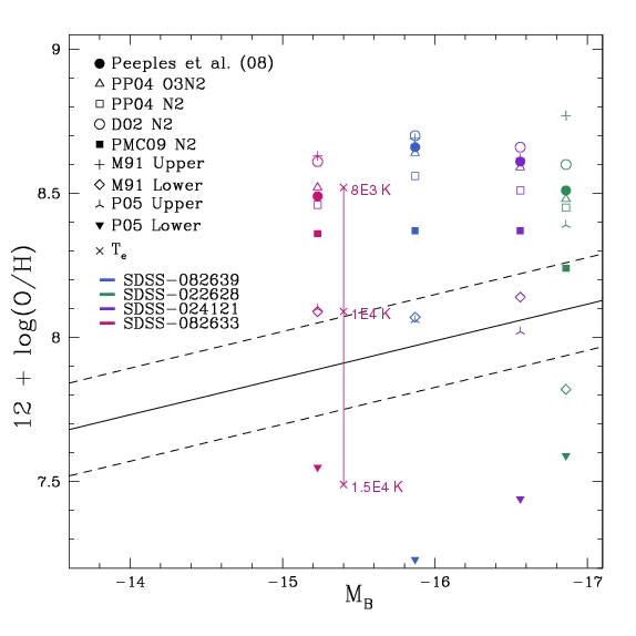
(a) Luminosity-Metallicity Relation

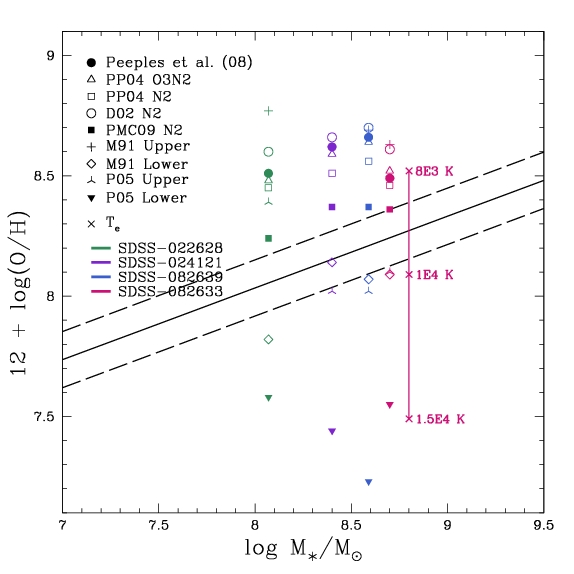
(b) Mass-Metallicity Relation

Figure 7: The figure (a) shows $12+\log(\mbox{O/H})$ vs. M_B for our sample. The solid line is the linear fit to dwarf galaxies found by Lee et al. (2006b) for comparison, with the dashed lines representing the 1 $\sigma$ uncertainty. This relationship is similar to that of van Zee et al. (2006b), but provides an average dispersion for both the L-Z and M-Z relationships. The points plotted display calculated oxygen abundances for our sample. Each method is denoted with a different symbol, where objects are differentiated by color: green for SDSS-022628, purple for SDSS-024121, blue for SDSS-082639, and pink for SDSS-082633. The ‘x’ symbols denote the oxygen abundances calculated from emissivities assuming various electron temperatures for SDSS-082633. Figure (b) displays $12+\log(\mbox{O/H})$ vs. $\log(\mbox{M}_{\star}/\mbox{M}_{\odot})$. Again, the solid line depicts the linear relationship and 1 $\sigma$ uncertainty of Lee et al. (2006b) for mass.

5.4 N/O Relative Abundances

Since many of the methods of abundance determination discussed here rely on N abundance values either to calibrate O/H values or to discriminate between bi-valued solutions, a confident measurement of the N abundance is important. Due to the relative insensitivity of the derived N/O ratio to electron temperature, it is possible to get a reliable estimate of this ratio in the absence of an electron temperature determination. We calculated the N/O values for our four galaxies (see Table 4), assuming that N⁺/O⁺ is approximately equivalent to that of N/O (based on their similar ratio of ionization potentials, Vila Costas & Edmunds, 1993) and an electron temperature of 12,500 $\pm$ 2,500 K.

The N/O versus O/H trend is well studied in galaxies of varying types. Vila Costas & Edmunds (1993) presented a thorough overview of theoretical expectations and observations available at the time. A salient point is that N can be produced as both a primary and a secondary element and that the secondary component is expected to be delayed relative to oxygen and to dominate at high abundances. Garnett (1990) convincingly demonstrated that there can be significant scatter in N/O at a given O/H, and Izotov & Thuan (1999) confirmed that this scatter is significant for oxygen abundances above 12 + log(O/H) = 7.7. Garnett (1990) proposed that much of the scatter could be explained by the time delay between producing oxygen and secondary nitrogen. However, Henry et al. (2006) conclude that the scatter in N/O could be produced by a variety of causes.

As already indicated in § 4, the four objects in our sample have unusually high values of N/O. PMC09 and, later, Amorín et al. (2010) (in their study of the abundances of the “green pea” galaxies) present a modern view of N/O versus O/H assembled from a sample of 475 H II objects and the SDSS DR7 catalog of observations respectively. A clear trend is obvious, but with scatter in log(N/O) on the order of 0.5 dex or more for a given O/H. An inspection of Figure 2 from Amorín et al. (2010) shows that our four galaxies, which range between $-0.8\leq$ log(N/O) $\leq-1.0$, correspond to values of 12 + log(O/H) $\approx$ 8.6 (derived from following the ridgeline of the data). Thus, empirically calibrated strong-line methods, such as O3N2 and N2, would predict oxygen abundances close to this value. However, the galaxies in this range of log(N/O) also extend to abundances as low as 12 + log(O/H) $\approx$ 7.9. From a plot of log(N/O) versus stellar mass for the SDSS compilation given by Amorín et al. (2010) (their Figure 3), our values of log(N/O) are roughly 0.6 dex higher than is typical for objects in the same stellar mass range.

5.5 Expected Oxygen Abundances

All strong-line calibrations correspond to an assumed electron temperature, so it is informative to explore the affects of varying this parameter. Since our MMT spectra include emission lines from both O⁺ and O⁺⁺, we can calculate an expected range in O/H values based on an assumed reasonable possible range in electron temperature. As an example, oxygen abundances were calculated for SDSS-082633 assuming electron temperatures of T${}_{e}=8\times 10^{3}$ K, $1\times 10^{4}$ K, and $1.5\times 10^{4}$ K. The resulting values of oxygen abundance cover the range of $12+\log(\mathrm{O/H})=7.5-9$, and are indicated by ‘x’ symbols in Figure 7; similar results are found for the other 3 galaxies. Thus, we cannot rule out any of the various strong line calibration estimates based on this consideration.

Finally, we can estimate the expected oxygen abundances from the luminosity-metallicity relationship and compare these to the strong line estimates in Figure 7. Each calibration is represented by a different symbol, and each of our four galaxies is designated with a different color. Using the M-Z relationship of van Zee et al. (2006b),

$$12+\log(\mbox{O/H})=5.67-0.151\ \mbox{M}_{B},$$ (4)

we calculate expected oxygen abundances of 8.22, 8.17, 8.07, and 7.97 for the four objects in our sample. The M-Z relationship found by Lee et al. (2006b), based on oxygen abundances obtained via the direct method and corroborated by Marble et al. (2010), covers the relevant range in luminosity for our sample and is also plotted in Figure 7. (Note that the range of the T04 relation does not extend down to encompass our low-luminosity sample). For each galaxy, a large spread is seen amongst the various indicators, highlighting the large uncertainties inherent in metallicity determinations.

Table 4: Estimates of the N/O Ratios for Our Sample

	log(N/O)
	MMT Data
Temperature	SDSS-022628	SDSS-024121	SDSS-082639	SDSS-082633
$1.00\times 10^{4}$ K	-0.94	-1.08	-0.98	-1.12
$1.25\times 10^{4}$ K	-0.80	-0.94	-0.84	-0.98
$1.50\times 10^{4}$ K	-0.70	-0.84	-0.74	-0.88
Adopted	-0.80 $\pm$ 0.12	-0.94 $\pm$ 0.12	-0.84 $\pm$ 0.12	-0.98 $\pm$ 0.12

Note. — N/O values for our four galaxy sample, calculated for a range of reasonable electron temperatures (12,500 $\pm$ 2,500 K).

6 DISCUSSION

6.1 Oxygen Abundances from Direct Comparison with Photoionization Models

The MMT spectra show that three of the objects observed have discrepantly low excitation (i.e., low $\lambda$5007/$\lambda$3727 ratio; log(O${}_{32})<-0.4$). This implies that the observed nebulae may have relatively low ionization parameters and/or be excited by an aging stellar population, which explains why we do not see other ions with high ionization potentials (such as He II $\lambda$4686) in our spectra. Since most strong line methods are calibrated for zero-aged main sequence starbursts, and many do not incorporate the effects of excitation, one must exercise care in applying these methods to determine oxygen abundances (see discussion in van Zee et al., 2006b). In general, the strong line methods tend to over-estimate the oxygen abundance for low excitation nebulae, and this offset can be as severe as $\sim$0.6 dex (van Zee et al., 2006b). Note that it may be possible to mitigate some error by combining empirical and theoretical determinations using an average as Moustakas et al. (2010) suggest.

Additionally, all four of the objects observed have relatively high values of N/O compared to systems of similar stellar mass. As discussed by Yin et al. (2007), PMC09, and Amorín et al. (2010), the assumption of a single relationship between N/O and O/H in photoionization model calibrations of the strong line methods can lead to discrepant results when the N abundance does not fit this assumed trend. At higher than average values of N/O, the strong line methods tend to over-estimate the oxygen abundance.

The combination of relatively low excitation and relatively high N/O values leads to a large bias in the results from the strong line calibrations. In Figure 8(a) we have plotted a comparison of the [O II] and [O III] line strengths for our four objects to photoionization models from Stasińska & Leitherer (1996). Each set of different colored points represents the evolution of a starburst assuming a Salpeter initial mass function (M${}_{up}=100$ M_⊙), a stellar mass between $10^{6}$–$10^{9}$ M_⊙, and a metallicity between 12 + log(O/H) = 7.33 and 8.93. Increasing symbol size denotes a progression from 1–10 Myr. These models are particularly valuable because they demonstrate the additional scatter that can be introduced as the exciting stars of an H II region age, and both the ionization parameter and shape of the ionizing spectrum evolve. Figure 8(a) shows that H II region models with oxygen abundances in the range of 7.9 $\leq$ 12 + log(O/H) $\leq$ 8.3 tend to have maximum values of R₂₃ (thus defining the turn-around regime in R₂₃; recall log(R₂₃) has an upper limit near 1.0). Our four spectra fall among the points for maximum R₂₃ at lower excitation. Figure 8(a) demonstrates that the four objects are inconsistent with relatively high (or relatively low) values of O/H, and, actually, are consistent with the values of O/H predicted from either the luminosity-metallicity relationship or the M-Z relationship.

Note that in constructing Figure 8(a), some of the Stasińska & Leitherer (1996) high-metallicity models showed more scatter in this diagram. These models included contributions by Wolf-Rayet (W-R) stars to the ionizing spectra, resulting in very hard radiation fields. We have not plotted these model points in Figure 8(a) because our non-detections of He II $\lambda$4686 indicate very little contribution from W-R stars at present.

MPA-JHU data for SDSS galaxies in the mass range of $7\leq$ log(M_⋆/M${}_{\odot})\leq 9$ are plotted in Figure 8(b) (gray points). Three of the four objects in the present sample, SDSS-024121, SDSS-082639, and SDSS-082633, are discrepantly low excitation nebulae relative to the SDSS sample, which tend to have higher excitation. However, most of the P08 “main” sample objects have ordinary excitation values. Note that seven of the 24 “main” sample objects did not have z $>0.024$ (consequently, they didn’t have [O II] $\lambda 3727$ in their spectra), and so could not be plotted here.

A complementary analysis is seen in Figure 9 where excitation (P) is plotted against log(R₂₃) for this same set of low mass SDSS galaxies (also see Moustakas et al. (2010) Figure 12 for a similar comparison). As discussed in § 5.3.3, three of our four objects lie well below the mean excitation for a given R₂₃ value. Figure 9 also shows an upper limit of log(R₂₃) naturally falls near 1.0, where the present sample lies within the turn-around region defined by $0.5\lesssim$ log(R${}_{23})\lesssim 1.0$, corresponding to 7.9 $\leq$ 12 + log(O/H) $\leq$ 8.3. A similar conclusion is drawn from the N2 calibration of PMC09 (§ 5.3.2) which suggests an oxygen abundance range of 8.30 $\leq$ 12 + log(O/H) $\leq$ 8.44 for the present objects based on the abnormal N/O variations present ($\sim 0.1-0.2$ dex less than other strong-line N2 calibrations). While we can’t constrain the oxygen abundance more precisely for this sample (based on the arguments here in § 6.1) than to put them in the range of 7.9 $\leq$ 12 + log(O/H) $\leq$ 8.4, this is sufficient to disqualify them as high-metallicity M-Z outliers.

Note that the recalibration of the O3N2 and N2 abundance indicators by PMC09 reduced the inferred oxygen abundances, but only by about half of what was needed to bring the objects in line with their expected abundances that we are proposing here. Even after recalibration, there is still a significant amount of scatter in these relationships. We speculate that taking into consideration the additional concern of low excitation would move these points further in the direction of concordance with expectations.

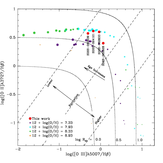
(a) Oxygen Abundance Models

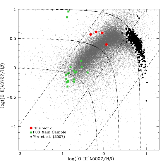
(b) Low-Mass SDSS Oxygen Abundances

Figure 8: (a) A comparison of the results from our MMT spectra with results from a large range of photoionization models evolved over 10 Myr as determined by Stasińska & Leitherer (1996) (symbol size corresponds to aging sequence). The overlaid dotted contours represent lines of constant R₂₃; from left to right log(R₂₃) = 0.0, 0.5, and 1.0. The turn-around region encompasses log(R₂₃) values of approximately 0.5 to 1.0. Dashed lines display excitation, where constant excitation of [O III]/[O II]= 1 coincides with the central line, [O III]/[O II]=0.1 is the low excitation line, and [O III]/[O II]=10 is the high excitation line. Our four spectra are all found near the maximum values of R₂₃ for relatively low excitation nebulae, indicating probable 12 + log(O/H) values in the range of 7.9 to 8.3. (b) Same plot of [O III] versus [O II] as Figure (a). The numerous gray dots are the MPA-JHU data for SDSS galaxies in the range of $7.0\leq$ log(M_⋆/M${}_{\odot})\leq 9.0$, which have higher excitation than SDSS-024121, SDSS-082639, and SDSS-082633. Values presented by Yin et al. (2007) for a sample of SDSS galaxies containing direct method abundances are also included for comparison. Notice that three of our objects from the “very low mass” sample are discrepantly low excitation relative to the SDSS and Yin et al. (2007) samples, whereas the “main” sample has ordinary excitation values for the most part.

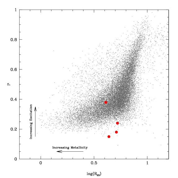
Figure 9: Excitation parameter P versus the metallicity sensitive R₂₃ index for the four objects in this paper (red dots) and the low-mass star-forming galaxies in the SDSS (gray dots). Arrows indicate direction of increasing excitation and increasing metallicity for the R₂₃ upper branch. For three of these objects, the excitation is rather low for their R₂₃ values.

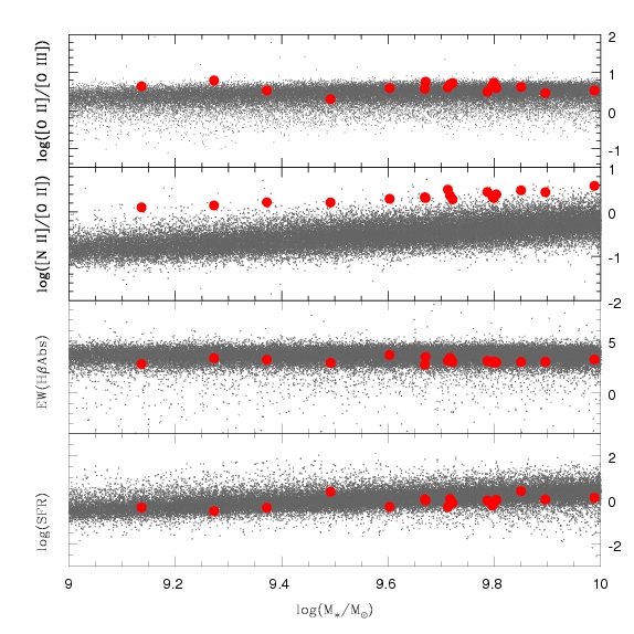
Figure 10: Properties of SDSS star-forming galaxies (gray dots) plotted against stellar mass ($9\leq$ log(M_⋆/M${}_{\odot})\leq 10$). In comparison, the P08 “main” sample (the 17 objects with measurable [O II]) are plotted in red. The top panel shows that in contrast to the “very low mass” sample, the “main” sample has normal ionization levels. Extremely high N values for the “main” sample relative to the SDSS average are shown in the second panel. The bottom two panels show that these objects have H$\beta$ absorption equivalent widths and SFRs congruent with the SDSS sample. As all objects in the P08 samples exhibit elevated N/O ratios, we suggest N enrichment is the prominent factor influencing these objects.

6.2 The True Nature of the High Oxygen Abundance Outliers

Although it appears that the “very low mass”, high oxygen abundance galaxies from P08 may not be true outliers from the M-Z relation, understanding how these galaxies produced spectra that lie far from the median relationships defined by the SDSS galaxies in various diagnostic diagrams remains an interesting question. Our MMT observations reveal that these spectra are characterized by (1) low excitation (low $\lambda$5007/$\lambda$3727 ratios; log(O${}_{32})<-0.4$, see Figures 8 and  9), (2) relatively high N/O abundance ratios for their stellar masses (see Figure 6), and (3) relatively deep underlying stellar Balmer absorption (ranging from 4 to 8 Å). All three characteristics can be explained by a previous, but recent burst of star formation. Essentially, these properties are all expected $\sim$ 5 Myr or longer after a starburst characterized as a “Wolf-Rayet galaxy.”

Kunth & Sargent (1981) demonstrated that the presence of strong W-R features in the spectrum of a star forming region are indicative of an intense episode of star formation lasting a relatively short (on the order of 10⁶ years) duration. For an instantaneous starburst, these W-R stars appear and disappear during the interval of 3 to 6 Myr (Leitherer & Heckman, 1995). Afterward, the most massive O stars have all evolved, and the less massive O and B stars produce a significantly softer spectrum resulting in lower excitation nebulae. The starburst models of González Delgado et al. (1999) show that the equivalent width of underlying stellar H$\beta$ absorption increases from roughly 2.7 to 4.5 Å as an instantaneous starburst of solar metallicity ages from 0 to 10 Myr, and continues on to nearly 9 Å at an age of 100 Myr. On this basis, the MPA-JHU estimates of the Balmer absorption are consistent with H II region ages greater than 4 Myr (3.4 Å), while our estimates (larger due to aperture differences), suggest a lower limit of 7 Myr (5.8 Å). Finally, during the W-R stage, it is possible for stars to release a large amount of N back into the local ISM (see, e.g., Esteban & Vilchez, 1992; Kobulnicky et al., 1997; López-Sánchez & Esteban, 2010, and references therein), producing inflated N/O ratios such as is seen in the four MMT spectra.

6.3 P08 “Main” Sample

Since all four of our objects, which were picked at random, have roughly identical spectral characteristics, we assume that the majority of the “very low mass” sample of P08 are probably similar. The “main” sample of P08 was defined by different restrictions, including a redshift cut to ensure the coverage of both [O II] and [O III] in the sample spectra (for 17 of the 24 “main” sample objects). We obtained the SDSS emission line strengths for the “main” sample from emission line analysis by the MPA-JHU collaboration. From these data we found the “main” sample galaxies (those with measured [O II] $\lambda 3727$) have normal $\lambda 3727/\lambda 5007$ ratios for their masses. In Figure 10 we show some the properties of the “main” sample relative to the SDSS parent sample, highlighting the normal ionization strengths in the top panel, followed by average H$\beta$ absorption equivalent widths and SFRs in the bottom two panels. The “main” and ‘very low mass” samples are different in that the “main” sample galaxies appear to have normal excitations. However, more importantly, in Figure 10 we have also plotted N/O ratio versus stellar mass for the P08 “main” sample, showing these galaxies all have very high N/O values. Similar to the four galaxies in our sample, the P08 “main” sample data suggest that they have also experienced recent N enrichment. Since high N/O values tend to bias strong line methods towards high abundances, and the metallicity offsets for the “main” sample are smaller than for the “very low mass” sample, this bias could easily account for most of this deviation.

All objects of the P08 parent sample display the characteristic nitrogen enhancement expected for a galaxy after passing through the “Wolf-Rayet galaxy” phase. P08 suggest that these objects are “transitional objects running out of fuel”: i.e., the high metallicity results because there is only a small amount of ISM to enrich. Our overall conclusion is that the high-metallicity outliers are special, not due to unusually high oxygen abundances for their mass or rate of star formation, but, rather, due to an enrichment of nitrogen relative to oxygen. This nitrogen enrichment may be due to being observed during a rare and short lived evolutionary phase.

7 CONCLUSION

We have investigated four of the 41 luminosity-metallicity outliers from the low-mass, high oxygen galaxy sample reported by Peeples et al. (2008). From new spectral observations taken at the MMT that include the [O II] $\lambda$3727 line, three of four galaxies were found to have relatively low excitation (low $\lambda$5007/$\lambda$3727 ratios; log(O${}_{32})<-0.4$) and, more importantly, all four exhibited high N/O values. Each of these characteristics can lead to overestimates of the oxygen abundance if standard strong line calibrations are used; furthermore, these two characteristics combined can produce the significant metallicity deviations seen for the P08 sample. By comparing our four spectra to the photoionization models of Stasińska & Leitherer (1996) (which include the effects of aging of the exciting stars), and the empirical calibrations of PMC09 (which correct for variations in the N/O ratio), we found that significantly lower oxygen abundances are favored. The Stasińska & Leitherer (1996) oxygen abundances are in line with those expected from the luminosities and stellar masses of the galaxies, while the PMC09 estimates shift oxygen abundances in the right direction. While the “very low mass” sample displays low star formation rates, the normal star formation within the “main” sample rules out exhaustive star formation as the variable responsible for the unusual sample spectra. With these conclusions, we propose that these galaxies are best described as nitrogen enriched, which may result from having recently passed through the “Wolf-Rayet galaxy” phase.

References

- Adelman-McCarthy et al. (2006) Adelman-McCarthy, J. K., et al. 2006, ApJS, 162, 38
- Alloin et al. (1979) Alloin, D., Collin-Souffrin, S., Joly, M., & Vigroux, L. 1979, A&A, 78, 200
- Amorín et al. (2010) Amorín, R. O., Pérez-Montero, E., & Vílchez, J. M. 2010, ApJ, 715, L128
- Bresolin (2007) Bresolin, F. 2007, ApJ, 656, 186
- Brinchmann et al. (2004) Brinchmann, J., Charlot, S., Heckman, T. M., Kauffmann, G., Tremonti, C., & White, S. D. M. 2004, arXiv:astro-ph/0406220
- Bruzual & Charlot (2003) Bruzual, G. & Charlot, S. 2003, MNRAS, 344, 1000
- Cardelli et al. (1989) Cardelli, J. A., Clayton, G. C., & Mathis, J. S. 1989, ApJ, 345, 245
- Charlot & Longhetti (2001) Charlot, S., & Longhetti, M. 2001, MNRAS, 323, 887
- Cooper et al. (2008) Cooper, M. C., Tremonti, C. A., Newman, J. A., & Zabludoff, A. I. 2008, MNRAS, 390, 245
- Contini et al. (2002) Contini, T., Treyer, M. A., Sullican, M., & Ellison, R. S. 2002, MNRAS, 330, 75
- Crawford & Barnes (1970) Crawford, D. L., & Barnes, J. V. 1970, AJ, 75, 978
- Dalcanton (2007) Dalcanton, J. J. 2007, ApJ, 658, 941
- Dekel & Silk (1986) Dekel, A., & Silk, J. 1986, ApJ, 303, 39
- Denicoló et al. (2002) Denicoló, G., Terlevich, R., & Terlevich, E. 2002, MNRAS, 330, 69
- Ellison et al. (2008) Ellison, S. L., Patton, D. R., Simard, L., & McConnachie, A. W. 2008b, AJ, 135, 1877
- Esteban & Vilchez (1992) Esteban, C., & Vilchez, J. M. 1992, ApJ, 390, 536
- Ferland et al. (1998) Ferland, G. J., Korista, K. T., Verner, D. A., Ferguson, J. W., Kingdon, J. B., & Verner, E. M. 1998, PASP, 110, 761
- Filippenko (1982) Filippenko, A. V. 1982, PASP, 94, 715
- Garnett (1990) Garnett, D. R. 1990, ApJ, 363, 142
- Garnett & Shields (1987) Garnett, D. R., & Shields, G. A. 1987, ApJ, 317, 82
- González Delgado et al. (1999) González Delgado, R. M., Leitherer, C., & Heckman, T. M. 1999, ApJS, 125, 489
- Henry et al. (2006) Henry, R. B. C., Nava, A., & Prochaska, J. X. 2006, ApJ, 647, 984
- Hummer & Storey (1987) Hummer, D. G., & Storey, P. J. 1987, MNRAS, 224, 801
- Izotov & Thuan (1999) Izotov, Y. I., & Thuan, T. X. 1999, ApJ, 511, 639
- Kauffmann et al. (2003) Kauffmann, G., et al. 2003, MNRAS, 341, 33
- Kennicutt et al. (2003) Kennicutt, R. C., Jr., Bresolin, F., & Garnett, D. R. 2003, ApJ, 591, 801
- Kewley & Ellison (2008) Kewley, L. J. & Ellison, S. L. 2008, ApJ, 681, 1183
- Kniazev et al. (2003) Kniazev, A. Y., Grebel, E. K., Hao, L., Strauss, M. A., Brinkmann, J., & Fukugita, M. 2003, ApJ, 593, L73
- Kobulnicky et al. (1999) Kobulnicky, H. A., Kennicutt, R. C., Jr., & Pizagno, J. L. 1999, ApJ, 514, 544
- Kobulnicky et al. (2003) Kobulnicky, H. A., et al. 2003, ApJ, 599, 1006
- Kobulnicky & Kewley (2004) Kobulnicky, H. A., & Kewley, L. J. 2004, ApJ, 617, 240
- Kobulnicky & Skillman (1996) Kobulnicky, H. A., & Skillman, E. D. 1996, ApJ, 471, 211
- Kobulnicky & Skillman (1997) Kobulnicky, H. A., & Skillman, E. D. 1997, ApJ, 489, 636
- Kobulnicky et al. (1997) Kobulnicky, H. A., Skillman, E. D., Roy, J.-R., Walsh, J. R., & Rosa, M. R. 1997, ApJ, 477, 679
- Kunth & Sargent (1981) Kunth, D., & Sargent, W. L. W. 1981, A&A, 101, L5
- Lee & Skillman (2004) Lee, H., & Skillman, E. D. 2004, ApJ, 614, 698
- Lee et al. (2006a) Lee, H., Skillman, E. D., & Venn, K. A. 2006a, ApJ, 642, 813
- Lee et al. (2006b) Lee, H., Skillman, E. D., Cannon, J. M., Jackson, D. C., Gehrz, R. D., Polomski, E. F., & Woodward, C. E. 2006b, ApJ, 647, 970
- Leitherer & Heckman (1995) Leitherer, C., & Heckman, T. M. 1995, ApJS, 96, 9
- Lequeux et al. (1979) Lequeux, J., Peimbert, M., Rayo, J. F., Serrano, A., & Torres-Peimbert, S. 1979, A&A, 80, 155
- López-Sánchez & Esteban (2010) López-Sánchez, Á. R., & Esteban, C. 2010, A&A, 517, A85
- Maiolino et al. (2008) Maiolino, R., et al. 2008, A&A, 488, 463
- Mannucci et al. (2010) Mannucci, F., Cresci, G., Maiolino, R., Marconi, A., & Gnerucci, A. 2010, MNRAS, 408, 2115
- Marble et al. (2010) Marble, A. R., et al. 2010, ApJ, 715, 506
- McCall et al. (1985) McCall, M. L., Rybski, P. M., & Shields, G. A. 1985, ApJS, 57, 1
- McCall (2004) McCall, M. L. 2004, AJ, 128, 2144
- McGaugh (1991) McGaugh, S. S. 1991, ApJ, 380, 140
- McGaugh (1994) McGaugh, S. S. 1994, ApJ, 426, 135
- Moustakas & Kennicutt (2006) Moustakas, J., & Kennicutt, Jr., R. C. 2006, ApJS, 164, 81
- Moustakas et al. (2010) Moustakas, J., Kennicutt, R. C., Jr., Tremonti, C. A., Dale, D. A., Smith, J.-D. T., & Calzetti, D. 2010, ApJS, 190, 233
- Oke (1990) Oke, J. B. 1990, AJ, 99, 1621
- Pagel et al. (1979) Pagel, B. E. J., Edmunds, M. G., Blackwell, D. E., Chun, M. S., & Smith, G. 1979, MNRAS, 189, 95
- Peeples et al. (2008) Peeples, M. S., Pogge, R. W., & Stanek, K. Z. 2008, ApJ, 685, 904
- Peeples et al. (2009) Peeples, M. S., Pogge, R. W., & Stanek, K. Z. 2009, ApJ, 695, 259
- Pettini & Pagel (2004) Pettini, M. & Pagel, B. E. J. 2004, MNRAS, 348, L59
- Pérez-Montero & Contini (2009) Pérez-Montero, E., & Contini, T. 2009, MNRAS, 398, 949
- Pilyugin et al. (2001a) Pilyugin, L. S. 2001a, A&A, 369, 594
- Pilyugin et al. (2001b) Pilyugin, L. S. 2001b, A&A, 373, 56
- Pilyugin & Thuan (2005) Pilyugin, L. S., & Thuan, T. X. 2005, ApJ, 631, 231
- Salim et al. (2007) Salim, S., et al. 2007, ApJS, 173, 267
- Savaglio et al. (2005) Savaglio, S., et al. 2005, ApJ, 635, 260
- Schlegel et al. (1998) Schlegel, D. J., Finkbeiner, D. P., & Davis, M. 1998, ApJ, 500, 525
- Schmidt et al. (1989) Schmidt, G. D., Weymann, R. J., & Foltz, C. B. 1989, PASP, 101, 713
- Shapley et al. (2004) Shapley, A. E., Erb, D. K., Pettini, M., Steidel, C. C., & Adelberger, K. L. 2004, ApJ, 612, 108
- Skillman et al. (1989) Skillman, E. D., Kennicutt, R. C., & Hodge, P. W. 1989, ApJ, 347, 875
- Skillman et al. (1996) Skillman, E. D., Kennicutt, R. C., Jr., Shields, G. A., & Zaritsky, D. 1996, ApJ, 462, 147
- Stasińska & Leitherer (1996) Stasińska, G., & Leitherer, C. 1996, ApJS, 107, 661
- Tremonti et al. (2004) Tremonti, C. A., Heckman, T. M., Kauffmann, G., Brinchmann, J., Charlot, S., White, S. D. M., Seibert, M., Peng, E. W., Schlegel, D. J., Uomoto, A., Fukugita, M., & Brinkmann, J. 2004, ApJ, 613, 898
- van Zee et al. (1998) van Zee, L., Salzer, J. J., Haynes, M. P., O’Donoghue, A. A., & Balonek, T. J. 1998, AJ, 116, 2805
- van Zee & Haynes (2006a) van Zee, L., & Haynes, M. P. 2006a, ApJ, 636, 214
- van Zee et al. (2006b) van Zee, L., Skillman, E. D., & Haynes, M. P. 2006b, ApJ, 637, 269
- Vila Costas & Edmunds (1993) Vila Costas, M. B., & Edmunds, M. G. 1993, MNRAS, 265, 199
- Vollman & Eversberg (2006) Vollmann, K., & Eversberg, T. 2006, Astronomische Nachrichten, 327, 862
- Yin et al. (2007) Yin, S. Y., Liang, Y. C., Hammer, F., Brinchmann, J., Zhang, B., Deng, L. C., & Flores, H. 2007, A&A, 462, 535
- York et al. (2000) York, D. G., et al. 2000, AJ, 120, 1579
- Zaritsky et al. (1994) Zaritsky, D., Kennicutt, Jr., R. C., & Huchra, J. P. 1994, ApJ, 420, 87