Study of Eclipsing Binary and Multiple Systems in OB Associations: I. Ori OB1a - IM Mon

Abstract

All available photometric and spectroscopic observations were collected and used as the basis of a detailed analysis of the close binary IM Mon. The orbital period of the binary was refined to 1.d19024249(0.00000014). The Roche equipotentials, fractional luminosities (in B, V and H_p - bands) and fractional radii for the component stars in addition to mass ratio $q$, inclination $i$ of the orbit and the effective temperature $T_{\rm eff}$ of the secondary cooler less massive component were obtained by the analysis of light curves. IM Mon is classified to be a detached binary system in contrast to the contact configuration estimations in the literature. The absolute parameters of IM Mon were derived by the simultaneous solutions of light and radial velocity curves as M${}_{\rm 1,2}=5.50(0.24)$ M_⊙ and 3.32(0.16) M_⊙, R${}_{\rm 1,2}=3.15(0.04)$ R_⊙ and 2.36(0.03) R_⊙, $T_{\rm eff1,2}=17500(350)$ K and 14500(550) K implying spectral types of B4 and B6.5 ZAMS stars for the primary and secondary components respectively. The modelling of the high resolution spectrum revealed the rotational velocities of the component stars as V${}_{\rm rot1}=147(15)$ km s^-1 and V${}_{\rm rot2}=90(25)$ km s^-1. The photometric distance of 353(59) pc was found more precise and reliable than Hipparcos distance of 341(85) pc. An evolutionary age of 11.5(1.5) Myr was obtained for IM Mon. Kinematical and dynamical analysis support the membership of the young thin-disk population system IM Mon to the Ori OB1a association dynamically. Finally, we derived the distance, age and metallicity information of Ori OB1a sub-group using the information of IM Mon parameters.

1 Introduction

Young stellar associations ($\leq$ 50 Myr) and open clusters have a crucial importance in advancing our understanding of star formation and the first stages of stellar evolution. Since the galactic acceleration does not have a chance to affect the kinematical properties of these young stellar groups, the stellar content of an association is preserved. Consequently one can obtain kinematical, dynamical and chemical properties of these young stellar groups by studying their secure members. Today nearby associations within the Solar neighbourhood have been very well identified. Their stellar content of each association has been precisely determined up to a magnitude limit of $V\sim$10.5 mag using astrometric data of the Hipparcos satellite (i.e. de Zeeuw et al., 1999; Hoogerwerf, 2000; Melnik & Dambis, 2009). In addition the new reduced Hipparcos catalogue (van Leeuwen, 2007) gave an opportunity to investigate the astrometric data of the stellar content of a large number of open clusters, associations and moving groups more accurately. The first application of the new reduced Hipparcos astrometric data is applied to stellar groups within the solar neighbourhood by Melnik & Dambis (2009). This and forthcoming studies of young stellar groups will improve our understanding of the history of star formation, the initial mass function, chemical and dynamical evolution of the Milky Way.

Recent statistical studies, such as Brown (2001), Bouy et al. (2006) and Kouwenhoven et al. (2007) show a high ratio of multiplicity in stellar formation regions (SFRs) and claim that it is not a coincidence, but a characteristic of star formation. The detailed study of multiple systems (especially those with eclipsing components) in SFRs will reveal the fundamental stellar parameters more directly and with higher precision compared to those obtained from single stars and thus impose more stringent tests on stellar evolution. Critical tests of stellar evolution require masses and radii with a precision better than 3 per cent (i.e. Andersen (1991); Torres, Andersen & Giménez (2010)). However, methods developed for single stars are not capable of delivering masses with a precision better than 5 per cent and radii remain uncertain by a factor of 1.5. Consequently studying single stars does not enable us to obtain accurate dimensions and, therefore, to test the most recent evolutionary models. Recent studies on $\eta$ Mus by Bakış et al. (2007) in Lower Centaurus-Crux association, on V578 Mon by Pavlovski & Hensberge (2000, 2005) in NGC 2244, and on AB Dor by Luhman & Potter (2006) in the AB Dor association, demonstrate the precision with which age, chemical composition and kinematical properties can be determined by studying such high-mass systems.

In the present study, we analyzed the high resolution spectra and BVH_p photometric data of IM Mon, which is located in the region of Ori OB1a association. IM Mon is a bright (V$\sim$6.5 mag), early-type ((B-V)=–0.14 mag) and short orbital period (P$\sim$1.2 days) eclipsing binary system. Its spectroscopic and photometric variations were discovered by Pearce (1932) and Gum (1951) respectively. The eccentricity of the spectroscopic orbit obtained by Pearce (1932) was commented to be spurious by Cester et al. (1978) in their study on the determination of photometric elements of 14 detached systems. Cester et al. (1978) studied early photometric observations of IM Mon, which were collected by Gum (1951) in integral light and by Sanyal, Mahra & Sanwal (1965) in $B$ and $V$ filters. However, due to a large scatter in all photometric observations, which is attributed to the intrinsic variability of one of the components by Sanyal, Mahra & Sanwal (1965), none of the authors was able to find a unique and precise solution for the system. A recent spectroscopic study of Bakış et al. (2010) revealed the spectroscopic orbital elements of IM Mon and showed that its orbit is circular.

In order to reveal more precise absolute dimensions of IM Mon and to test its membership to Ori OB1a, we included it into our list of eclipsing binaries in the region of OB associations. Using all literature based data the orbital period of IM Mon is revised in §2.3. High resolution spectral lines of IM Mon are modelled and atmosphere parameters are derived in §3. The close binary stellar parameters of the system are determined by the analysis of light and radial velocity (RV) curves in §4. In §5 the absolute parameters of the components are derived together with the age and distance of the system. This information enabled us to establish the absolute dimensions of the close binary and properties of the Ori OB1a association through the kinematical and dynamical properties of IM Mon. Finally we summarized our study and present our conclusions in §6.

2 Observational Data

We collected as many original individual measurements of IM Mon as possible from the literature. In table 1, all available photometric and spectroscopic observations of IM Mon are listed. All the data given in table 1 are used for ephemeris determination for O–C analysis, whereas only relatively more precise photometric data are used for light curve (LC) modelling. As a starting orbital period, we adopted $P=1\timeform{d}.1902424$, which is published by Kreiner (2004) and later used by Bakış et al. (2010) for their radial velocity analysis.

Table 1: List of sources of measurements used (after removing outliers). C(B) and C(R) stand for clear filters with B and R effective bands, respectively.

No.	Source	Filter	No. of points	$\sigma$	Notes
Photometry				[mmag]
1	Gum (1951)	C(B)	33	3.7	normal points
2	Sanyal et al. (1965)	B	42	3.4	normal points
3		V	41	4.4	normal points
4	Shobbrook (2004)	V	40	7
5	Hipparcos	Hp	118	6
6		$V_{\rm{T}}$	159	38
7		$B_{\rm{T}}$	159	41
8	ASAS	V	435	26
9	Pi	C(R)	490	32
Spectroscopy				[km s-1]
10	Pearce (1932)	RV	18	29	primary
10	Pearce (1932)	RV	13	41	secondary
11	Bakış et al. (2010)	RV	23	13	primary
11	Bakış et al. (2010)	RV	20	16	secondary

2.1 Photometric Data

• Gum (1951) – Data were obtained with nine-inch refractor of the Commonwealth Observatory, Canberra equipped with a photoelectric photometer with 1P21 photomultiplier tube on effective wavelength 440.0 nm (without filter) in one season 1949-1950 (normal points related to JD 2 433 402); HD 45321, HD 44756 were used as comparison stars.

• Sanyal & Sinvhal (1964) – B and V observations of UBV system (Johnson and Morgan 1951) were made during 29 nights of three seasons in 1960-1964 (normal points related to JD 2 438 384) at Uttar Pradesh State observatory, Naini Tal using 10 inch Cooke refractor and 15-inch reflector equipped with unrefrigerated 1P21 photomultiplier. BD -2^∘ 1601 (=HD 45139) and BD -3^∘ 1414 (=HD 44720) were used as comparison and check stars respectively.

• Shobbrook (2004) – The 24-inch (61-cm) telescope of the Australian National University at Siding Spring Observatory with photometer – a cooled GaAs photomultiplier and the Motorised Filter Box with Strömgren $y$ and b filters were used in JD 2 450 458–2 452 026. The observations were reduced to the Johnson V scale using $uvby$ secondary standard stars of Cousins (1987) in the E Regions (sic). HR 2325 (=HD 45321) and HR 2344 (=HD 45546) were used as comparison stars.

• Hipparcos (ESA, 1997) – Observations were made by Hipparcos satellite equipment (reflector 29-cm, f=1.4-m) in the interval JD 2 447 960–2 449 058. More details are on webpage.

• ASAS (Pojmański, 1997) – Observations were obtained from two ASAS observing stations, one is in Las Campanas Observatory, Chile (since 1997) and the other is on Haleakala, Maui (since 2006) between JD 2 452 731–2 455 167. Both were equipped with two wide-field instruments (72-mm, f=0.2-m), observing simultaneously in V and $I$ band. However, only V measurements are available for IM Mon. More details and data archive are on webpage.

• Pi of the Sky (Małek et al., 2010) – The Pi of the Sky robotic telescope has been designed for monitoring of a significant fraction of the sky with good time resolution and range. Final detector consists of two sets of 16 cameras, one camera covering a field of view of 20${}^{\circ}\times 20^{\circ}$. The final system is currently under construction. Required hardware and software tests have been performed with a prototype located in Las Campanas Observatory in Chile since June 2004. The set of IM Mon measurements cover time the interval of JD 2 453 954–2 454 946. More details and data archive are on webpage.

2.2 Spectroscopy

• Pearce (1932) – 19 spectrograms were obtained at Dominion Astrophysical Observatory using a 72-inch telescope in the interval JD 2 424 942–2 425 682, mostly with the short-focus camera having a dispersion 49 Å/mm at H$\gamma$. From these spectrograms, a total of 31 RVs (18 for primary and 13 for secondary component) have been measured by Pearce (1932). We used all RVs given by Pearce (1932) in this study.

• Bakış et al. (2010) – The spectra were taken with High Efficiency and Resolution Canterbury University Large Echelle Spectrograph (HERCULES) of the Department of Physics and Astronomy, New Zealand. It is a fibre-fed échelle spectrograph, attached to the 1-m McLellan telescope at the Mt John University Observatory (MJUO). All spectra were collected using the 4k $\times$ 4k Spectral Instruments 600S CCD camera. All 23 spectra were obtained in August 2006 (JD 2 453 981-2 453 992). A detailed description including journal of observations is given in Bakış et al. (2010).

  Bakış et al. (2010) used a two-dimensional cross-correlation technique for measuring RVs of the components of IM Mon, whose spectra show evidently blended lines at specific orbital phases. This technique is more suitable for the measuring RVs of close binary systems in the case of blended spectral lines at some phases, though is not as powerful as spectra disentangling (Simon & Sturm, 1994; Hadrava, 1995). However, due to very strong blending near the eclipse phases when the eclipsed component’s spectral lines are invisible, it was not possible for them to measure a reliable RV of the secondary component at four phases (Bakış et al., 2010). Notice that in table 2 of Bakış et al. (2010), the listed RVs are uncorrected for barycentric motion although the spectroscopic orbital elements given were obtained from the corrected RVs. Herewith we re-list the corrected RVs in table 2.

Table 2: RVs of IM Mon. Orbital phases ($\varphi$) were calculated using the same ephemeris given by Bakış et al. (2010).

No	HJD	Phase	RV1	(O-C)1	RV2	(O-C)2
	(-2453900)	($\varphi$)	(km s-1)	(km s-1)	(km s-1)	(km s-1)
1	81.1889	0.866	133.2	8.8	-153.4	-2.7
2	81.2155	0.888	121.4	11.8	-131.4	-5.2
3	81.2402	0.909	118.0	21.8	-96.5	7.6
4	82.2019	0.717	160.2	4.9	-206.5	-4.9
5	82.2313	0.742	165.7	7.3	-197.7	9.0
6	85.1955	0.232	-112.7	3.7	252.4	5.6
7	86.1892	0.067	5.9	40.9	-	-
8	86.2328	0.104	-43.9	19.6	139.7	-30.4
9	86.2442	0.113	-51.1	18.8	151.4	-18.7
10	88.1948	0.752	163.1	4.5	-203.8	3.2
11	88.2354	0.786	161.0	5.8	-203.4	-1.9
12	89.1573	0.561	53.2	-19.3	-	-
13	89.1868	0.585	91.6	4.1	-112.2	-16.4
14	89.2141	0.608	115.5	7.3	-135.4	-11.5
15	89.2404	0.631	123.0	1.2	-162.0	-15.6
16	90.1456	0.391	-69.5	-2.6	147.8	-17.2
17	90.1730	0.414	-52.6	-0.9	111.5	-13.4
18	90.2098	0.445	-7.4	19.9	-	-
19	91.1578	0.241	-120.0	-2.9	237.9	-10.0
20	91.2020	0.279	-103.7	11.6	253.8	9.0
21	92.1558	0.080	-57.4	-11.2	119.2	-11.5
22	92.2077	0.123	-76.5	-0.4	202.8	22.6
23	92.2390	0.150	-82.1	9.0	212.7	7.8

3 Modelling Spectral Lines

We have modelled the spectral orders extracted from a high resolution échelle spectrum of IM Mon with the theoretical atmosphere models of Kurucz (1993) to obtain the atmosphere parameters such as metallicity $[Fe/H]$, effective temperature ($T_{\rm eff}$), surface gravity ($\log g$), projected rotational velocity (V_rot sin$i$) and microturbulance velocity ($\zeta$) of the components. These atmosphere parameters, especially the metallicity, which can be obtained primarily from the observed spectrum, are very useful during the construction of the isochrones of IM Mon. The atmosphere models we used are originally provided for a wide range of temperature, surface gravity and metallicity by Kurucz (1993). For specific values of these parameters, one should use routines to obtain desired atmosphere parameters. We used ATLAS9 and SYNTHE routines (Kurucz, 1993) with new opacity distribution functions (ODF) provided by Castelli & Cacciari (2001). In order to find the best fitting atmosphere parameters, the Grid-Search Method (Bevington, 2003) was used. The Grid-Search Method is based on minimization of the following $\chi^{2}$ by changing the fitting parameters (x_i) with their increments $\Delta$x_i,

$$\chi^{2}=\sum_{i=1}^{N}\left(\frac{y_{i}-y([Fe/H],T_{\rm eff},\log g,V_{rot}sin(i),\zeta)}{\sigma_{i}}\right)^{2},$$ (1)

where $y_{i}$ denotes the observed quantities, $y(x_{i})$ are the calculated models as a function of atmosphere parameters and $\sigma_{i}$ is the standard deviation of the observed spectrum with $N$ data points. Since the wavelength range of spectral orders we study are relatively small ($\langle$100 Å), we assume that the standard deviation along the spectral order remains the same ($\sigma^{2}_{i}$=$\sigma^{2}$) and is related with the S/N ratio of the spectrum with $\sigma^{2}=\frac{1}{(S/N)^{2}}$. Uncertainties of the model parameters are estimated from the standard deviation of the parameters, which are obtained for each spectral order, from the mean.

A grid of atmosphere models has been constructed for the following ranges of $[Fe/H]=[-0.04,0.20](0.04)dex$, $T_{\rm eff1}$ = [16000, 19000] (200) K, $T_{\rm eff2}$ = [13000, 15000] (200) K, $\log g_{\rm 12}$ = [4.0, 4.3] (0.1) cgs, $\zeta_{\rm 12}$ = [2, 4] (1) km s^-1, V_rot1 sin$i$= [110, 150] (5) km s^-1 and V_rot2 sin$i$= [60, 100] (5) km s^-1 with the increments given in brackets. In order to shrink the parameter space in Eq. 1, the metallicity and microturbulance velocity intervals are adopted from the spectroscopic study of four B-type Ori OB1a members (Cunha & Lambert, 1994) and statistical study of B-type stars (Nieva & Przybilla, 2010; Kodaira & Scholz, 1970) respectively. The effective temperature intervals are determined using the colour information of the system (see §4.1). Surface gravity and projected rotational velocity intervals are adopted from the components’ spectral types which are estimated from their temperatures and mass functions obtained from the spectroscopic orbit by Bakış et al. (2010).

The normalized flux of the LC of IM Mon at out of eclipses is changing with phase due to the elongated shapes of the component stars and due to the reflection effect, which causes a variation in the contribution factor of the components in the total light, therefore in the composite spectrum. In the eclipse phases, a light dilution of the eclipsed component should also be taken into account as an additional effect on the light contributions. Therefore, the most suitable orbital phases to study the spectral lines of the components in a binary system with circular orbit are the quadrature phases, where components’ spectral lines are the strongest and well-seperated, unless there is a total eclipse in the system. In case of a total eclipse, the most suitable phase to study the eclipsing component is the middle of the eclipse phase, where the totally eclipsed component has no light contribution to the total light. In our case, before fitting the models to the observed spectrum at a chosen orbital phase ($\phi$=0.75), the synthetic spectrum of the components is re-scaled by considering their light contribution in each photometric band listed in table 4. For the spectroscopic regions different from the effective wavelengths of the photometric bands of the observations (BVH_p), an interpolation of the light contributions for a specific wavelength of the spectral line being analyzed is applied. The Doppler shifts of the components due to the orbital motion are also calculated using the orbital parameters given in table 4 of Bakış et al. (2010) and this shift is applied to the synthetic spectrum of the component stars before forming the composite spectrum.

The continuum normalization procedure is also an important factor since a wrong normalization may alter the line depths leading to an additional uncertainty in the modelling parameters. Toward the early-type stars, the continuum is more visible due to a decreasing number and strength of neutral metallic lines. However, the fast rotation of early-type stars also has a negative effect on the visibility of the continuum. Therefore, those studying early-type stellar spectrum are luckier than those studying late-type stars in the sense of determination of continuum regions of the spectrum. The general procedure of continuum normalization of IM Mon spectra is already given by Bakış et al. (2010). To estimate uncertainty raising from continuum normalization, each spectral order is nomalized five times and the resulting line depths of the spectral lines are investigated. The standard deviation of measured line depths is of the order of 0.1 per cent which is in the uncertainty box of an observed spectrum with average S/N ratio of 100. Therefore, uncertainties in our model parameters are mostly due to the bias of the spectrum rather than the continuum normalization procedure.

All spectral lines which are clearly visible in the observed spectrum and are given in table 3 are analyzed. Atmospheric parameters obtained from metallic lines are consistent for both components while for Balmer and helium lines of the primary component a discrepancy between model and observations is noticed. This is because of the fact that starting from late B type stars (T_eff $>$ 15000 K) there is a discrepancy between the non-LTE and LTE models for neutral helium and Balmer lines, which progressively becomes more important as the effective temperature of the star increases (O’Mara & Simpson, 1972). Nevertheless, the discrepancy between LTE and non-LTE for metallic lines is negligible (Nieva & Przybilla, 2007). The inconsistency of atmospheric parameters from the metallic lines and the helium lines is due to the departure from LTE for the primary component which is negligible or undetectable for the secondary component because of its lower temperature. Since our atmosphere calculations are all LTE-based, we conclude that the modelling of Balmer and helium lines of the primary component can not be performed with our adopted LTE atmosphere models. However, the existance of the metallic lines of the primary in the spectrum is still adequate for the determination of its atmosphere parameters. Therefore, we used only metallic lines given in table 3 for finding the best fitting atmosphere parameters. The best fitting model spectrum is shown in figure 1.

The modelling of the observed spectrum yielded the following atmosphere parameters with their uncertainties in brackets for the components of IM Mon; T_eff1 = 17500(350) K, T_eff2 = 14500(450) K, $\log g_{\rm 1}$ = 4.20(0.10) cgs, $\log g_{\rm 2}$ = 4.20(0.10) cgs, $\zeta_{\rm 12}$ = 2(2) km s^-1, $V_{\rm{rot}1}\sin i=130(10)$ km s^-1, $V_{\rm{rot}2}\sin i=80(20)$ km s^-1 and $[Fe/H]=0.20(0.15)$ dex.

For comparison with the best fitting atmosphere model, we computed two more synthetic spectra: one with the solar metallicity and one with the atmosphere parameters varied by 1-$\sigma$, both are shown in figure 1. The atmosphere parameters varied by 1-$\sigma$ are T_eff1 = 17150 K, T_eff2 = 14050 K, $\log g_{\rm 1}$ = 4.10 cgs, $\log g_{\rm 2}$ = 4.10 cgs, $\zeta_{\rm 12}$ = 0 km s^-1, $V_{\rm{rot}1}\sin i=120$ km s^-1, $V_{\rm{rot}2}\sin i=60$ km s^-1 and $[Fe/H]=0.35$ dex.

The derived metallicity ($[Fe/H]=0.20(0.15)$ dex) is just at the edge of the grid range, but the value is well-determined because the test calculation for comparison with 1-$\sigma$ variation (see figure 1) shows a large difference between observed and theoretical spectra.

Table 3: Spectral lines visible in the observed spectrum of IM Mon.

Spectral Order	Spectral Line	Wavelength (nm)
85	He I	667.8
87	Hα	656.3
89	Ne I	640.2
	Si II	637.1
90	Si II	634.7
97	He I	587.5
101	S II	564.7
		564.6
		564.0
104	Si II	546.7
	Fe II	546.6
	S II	545.4
113	He I	504.8
	Si II	504.1
	C II	503.2
	He I	501.6
116	S II	492.5
	Fe II	492.4
	He I	492.2
121	He I	471.3
127	Mg II	448.1
	He I	447.2
130	He I	438.8
133	S II	426.8
137	He I	414.4
141	He I	402.6

(60mm,60mm)figure1a.eps	(60mm,60mm)figure1b.eps
(60mm,60mm)figure1c.eps	(60mm,60mm)figure1d.eps
(60mm,60mm)figure1e.eps	(60mm,60mm)figure1f.eps
(43mm,60mm)figure1g.eps

Figure 1: Observed composite spectrum of IM Mon at orbital phase $\phi$=0.75 and the model spectrum Doppler shifted and re-scaled for the light contributions of the component stars. The synthetic spectrum calculated for solar metal abundance and for atmosphere parameters varied by 1-$\sigma$ are also shown for comparison. In each panel the dashed-dotted lines are the observed spectrum whereas the solid, dashed and dotted lines (only in top right panel) stand for the best fitting, solar metal abundance and 1-$\sigma$ varied synthetic spectrum (only for Si II 634.7 nm line), respectively. The normalized $\chi^{2}$ variation of primary star temperature in our grid search is shown at the bottom.

4 Close Binary Stellar Parameters

4.1 Binary Model and Input Parameters

Accurate estimation of the primary star temperature is one of the most critical tasks before the LC modelling of close binary stars. A wrong estimation affects the determination of the secondary star’s temperature which leads to incorrect evolutionary scenarios. In this study two methods are used for temperature estimation, a) by modelling spectral lines and b) by the $Q$-method of Johnson & Morgan (1953) using the $UBV$ colours of IM Mon. The modelling of spectral lines is already discussed in §3 and the primary star temperature is found to be T${}_{\rm eff1}=17500$ K. The $Q$-method of Johnson & Morgan (1953) is based on linear correlation between the reddened and unreddened coulor of stars as the following relation:

$$Q=(U-B)-\frac{E(U-B)}{E(B-V)}(B-V),$$ (2)

where $(U-B)$ and $(B-V)$ are the reddened colour indices and $E(U-B)$ and $E(B-V)$ are colour excesses in these indices respectively. Johnson & Morgan (1953) determined the mean value of $\frac{E(U-B)}{E(B-V)}$ to be 0.72$\pm$0.03 from the unreddened and reddened stars tabulated in their study. Since the linear correlation between the reddened and unreddened colours is valid for early-type stars, the usage of the $Q$-method is limited for the spectral type range B1-B9 which corresponds to range in the $Q$ parameter as –0.80$<Q<$–0.05. Once the $Q$-parameter is obtained, the unreddened colour index $(B-V)_{0}$ can be derived from $(B-V)_{0}=-0.009+0.337Q$. Using the unreddened colour index of $(B-V)_{0}$, one can derive the colour excess of $E(B-V)$ from $E(B-V)$=$(B-V)_{0}-(B-V)$. The unreddened colour excess $E(U-B)$ can also be derived from the relation $\frac{E(U-B)}{E(B-V)}=0.72\pm 0.03$. Then the unreddened colour index of $(U-B)_{0}$ is found from $E(U-B)$=$(U-B)_{0}-(U-B)$.

The combined colours of IM Mon were collected from Deutschman, Davis & Schild (1976) as $(U-B)=-0.650(0.013)$ and $(B-V)=-0.150(0.019)$. The combined colour of IM Mon yielded the $Q$-parameter $Q=-0.542\pm 0.03$, colour excess $E(B-V)=0.042$$\pm$0.033 and visual absorption $A_{\rm v}=0.129$. Therefore, the unreddened colours of the system are $(B-V)_{0}=$ –0.192$\pm$0.014 mag and $(U-B)_{0}=-0.680$$\pm$0.039 mag. These unreddened colours correspond to a temperature of 17000$\pm$200 K according to the calibration tables of Cramer (1984). However, it should be noted that these colours and the corresponding temperature are obtained from the combined light of the components, resulting in a slightly redder colour and lower temperature than the intrinsic colour of the primary component, although the LCs and the spectral lines show that the light of the primary star dominates. Since the spectral line modelling yields intrinsic temperatures of the component stars, we adopted a temperature of T_eff1=17500 K$\pm$350 K for the primary star.

4.2 Determination of the Photometric Elements

From table 1, where all available photometric data of IM Mon are listed, five photometric data sets (B band data of Gum (1951), B and V band data of Sanyal et al. (1965), V band data of Shobbrook (2004) and H_p band data of Hipparcos) are selected for simultaneous analysis of LCs together with the RVs of the components using the 2003 version of the Wilson-Devinney LC analysis code (Wilson & Devinney, 1971; Wilson, 1994). Selection was made according to their relative precision among others.

Using the best data specified above we obtained the estimate of the period $P$ and initial epoch of primary minimum $M_{0}$ together with the model LCs in various colours and model RV curve. We then found that there are systematic seasonal differences between the observed and the model LCs. The seasonal LC variations were already mentioned by Sanyal & Sinvhal (1964) who observed the system extensively during 1962–1964. They found that the scatter seen in the light curve of IM Mon is not random but systematic due to intrinsic variability of the cooler component. The authors argued that the period of these variations is nearly, but not exactly, equal to half of the orbital period. Such type of variability should then manifests itself in long-term changes in the shape of LC in individual observational sets.

The presence of LC changes is clearly apparent in Fig.2 depicting the difference between observed LCs and the mean LC. The double-wave character of these differential LCs supports the findings of Sanyal & Sinvhal (1964), however their hypothesis on the intrinsic variability of the cooler component is not unique. Observed seasonal LCs changes resemble those ones found in the non-eclipsing interacting binary HD 143 418 containing a subsynchronously rotating primary passing through its synchronization stage. The seasonal variability of the orbitally modulated light curves is related to an expected incidence of circumstellar matter originating in the tidally spinning up primary component (Bozic et al., 2007; Zverko et al., 2009). This makes the more detailed study of seasonal changes of IM Mon appealing.

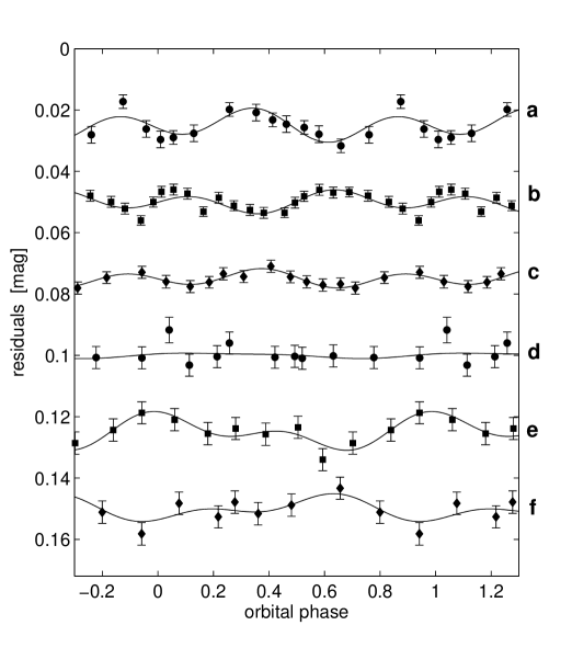
Figure 2: Seasonal variability of light curve shapes visualized through the difference of an individual observed light curve defined by their normal points and mean light curve. a – Gum (1951), b – Sanyal, Mahra & Sanwal (1965), c – ESA (1997), d – Shobbrook (2004), e – Pojmański (1997), f – Małek et al. (2010).

Aiming to restrain the influence of seasonal variations we corrected all observed data by approximating the data by the double wave harmonic function. The scatter of residuals then diminished considerably. Subsequently, the new model phase curves were used as templates that were applied to all the observational data summarized in the table 1 with the aim to compute improved ephemeris.

The procedure is iterative, assuming that $y_{i}$ is $i$-th measurement obtained in the time $t_{i}$, $F(\vartheta(t_{i}))$ is the model prediction for the $i$-th measurement and $w_{i}$ is its weight (inversely proportional to the square of its assumed uncertainty). $\vartheta(t_{i})$ is then the so-called phase function (the fractional part of it being the common phase $\varphi$, the integer part is the epoch $E$). The linear phase function is determined by the simple relation: $\vartheta(M_{0},\,P,\,t)=(t-M_{0})/P$, where $M_{0}$ is the time of initial epoch of primary minimum and $P$ is the orbital period. We found parameters $P$ and $M_{0}$ so that the following is valid:

$$\Delta y_{i}=y_{i}-F(\vartheta(t_{i})),\quad\sum_{i=1}^{n}\Delta y_{i}\frac{\partial F}{\partial\vartheta_{i}}\,w_{i}=0\ \textrm{and}\ \sum_{i=1}^{n}\Delta y_{i}\frac{\partial F}{\partial\vartheta_{i}}\vartheta_{i}\,w_{i}=0.$$ (3)

After several iterations we obtained the following equation for heliocentric data of the primary minima:

$$\mathrm{HJD_{I}}=M_{0}+P\,E=2\,442\,331.2515(9)+1\timeform{d}.19024249(14)\,E,$$ (4)

where $E$ is an epoch number.

The orbital period $P=1\timeform{d}.19024249(14)$ given in eq. 4 agrees with the period $P=1\timeform{d}.1902424$ found by Kreiner (2004). Nevertheless, the present value of the orbital period is more reliable and precise because it is based on much larger observational material and on their more careful treatment.

Supposing a non-zero but constant time derivative of the period $\dot{P}$ we found a moderate increase of the orbital period of $\dot{P}=(9\pm 5)\times 10^{-11}$, which may not be real.

The orbital period ($P$) and the initial epoch of the primary minimum ($M_{0}$) were kept fixed during the simultaneous solutions. Since the time derivative of the orbital period ($\dot{P}$) is statistically not significant, its value is taken to be zero as the fixed parameter. The temperature of the primary was fixed at $T_{\rm eff1}$ = 17500 K and the temperature of the secondary ($T_{\rm eff2}$) was left to converge. Gravity darkening exponents $g_{\rm 1}=g_{\rm 2}=1$ and bolometric albedos $A_{\rm 1}=A_{\rm 2}=1$ were set for radiative envelopes (von Zeipel, 1924). The logarithmic limb-darkening law was used and limb-darkening coefficients were taken from van Hamme (1993). The surface potentials ($\Omega_{\rm 1,2}$), light factors of the components ($l_{\rm 1,2}$), orbital inclination ($i$), the mass ratio ($q$), seperation ($a$) of the components and the systemic velocity ($V_{\gamma}$) were the adjusted parameters during the modelling of the LCs. The orbital eccentricity ($e$) and longitude of periastron ($\omega$) were fixed for a circular orbit (Bakış et al., 2010).

In addition to the LC input parameters given above, the solution mode, which describes the type of the binary (i.e. detached binary, semi-detached binary, contact binary), is required by the Wilson-Devinney code as program input. The most recent photometric analysis of IM Mon by Cester et al. (1978) was not succesfull to classify the type of the binary due to large scatter in the photometric data they used. Nevertheless, Pourbaix et al. (2004) emphasized the possibility of contact status of the system in “SB9: The ninth catalogue of spectroscopic binary orbits ”. We, therefore, initially tested all possible solution modes (Mode 2 for detached binaries, Mode 3 for overcontact binaries with components having different surface brightnesses, Mode 4 and 5 for semi-detached binaries and Mode 6 for double contact binaries) with the Wilson-Devinney code. None of the solutions with contact and semi-contact configurations converged to give a good fit and in each trial the fitting parameters converged to a detached configuration. Hence, in the following steps of the analysis, detached binary configuration has been adopted.

The solutions with detached configuration in each photometric band converged very rapidly, and had the smallest residuals. Input values of the adjusted parameters and the primary star temperature were then altered to check the consistency and uniqueness of the solution. A change in the value of primary star temperature did not affect other parameters’ output values significantly except for the secondary star temperature. These new input parameters converged to the parameters of the first solution, which shows the consistency of the solutions listed in table 4. The uncertainties of the final light curve modelling parameters (see table 4) directly come from the light curve modelling program output. Adopted LC solutions for each photometric set are shown in figure 3 together with RV solutions and the star shapes at four different orbital phases. The Rossiter-McLaughlin effect seen near the eclipse phases of close binary systems is very small in the case of IM Mon due to the low inclination of its orbit (see star shapes at eclipses in figure 3). However, near the primary eclipse, there is one of the RVs of the primary component significantly outlying from the theoretical curve. This RV is clearly not measured precisely due to the blending of the spectral lines at this phase and the scatter is certainly not due to Rossiter-McLaughlin effect since it is red-shifted.

Table 4: Results from the simultaneous solution of B, V and Hp-band LCs of IM Mon system. Adjusted and fixed parameters are presented in separate panels of the table. Uncertainties of adjusted parameters are given in brackets.

Parameter	Value
Adjusted parameters:
$T_{\rm eff2}(K)$	14500(200)
$L_{1}/L_{1+2}(B)$	0.700(0.003)
$L_{1}/L_{1+2}(Hp)$	0.698(0.005)
$L_{1}/L_{1+2}(V)$	0.693(0.002)
$\Omega_{\rm 1}$	3.75(0.12)
$\Omega_{\rm 2}$	3.72(0.08)
$\Omega_{\rm cr}$	3.07
$r_{\rm 1}$(mean)	0.323(0.020)
$r_{\rm 2}$(mean)	0.242(0.030)
$i(^{o})$	62.2(0.9)
$q$	0.603 (0.011)
$a(R_{\odot})$	9.77 (0.14)
$V_{\gamma}$ (km s-1)	22.1(2.1)
Fixed parameters:
$P$	1$\timeform{d}$.19024249
$\dot{P}$	0.0
$M_{0}$	2 442 331.2515
$e$	0.0
$A_{1}=A_{2}$	1.0
$g_{1}=g_{2}$	1.0
$T_{\rm eff1}(K)$	17500
x${}_{\rm 1}(B,V,H_{p})$	0.516, 0.438, 0.462
y${}_{\rm 1}(B,V,H_{p})$	0.279, 0.234, 0.249
x${}_{\rm 2}(B,V,H_{p})$	0.561, 0.478, 0.504
y${}_{\rm 2}(B,V,H_{p})$	0.303, 0.254, 0.269
$F_{\rm 1}$=$F_{\rm 2}$	1.0
$\chi^{2}_{\rm min}(B_{1},B_{2},V_{1},V_{2},H_{p})$	0.0029, 0.0032, 0.0039, 0.0056, 0.0042
$B_{1}$ (Gum, 1951), $B_{2}$ (Sanyal et al., 1965),
$V_{1}$ (Sanyal et al., 1965), $V_{2}$ (Shobbrook, 2004), $H_{p}$ (ESA, 1997).

(80mm,80mm)figure3a.eps

(90mm,90mm)figure3b.eps

(80mm,80mm)figure3c.eps

Figure 3: Theoretical model fits to five different photometric band LCs (top) and RV data (middle) of IM Mon. The star shapes are plotted for different orbital phases (bottom).

5 Results and Discussion

5.1 Astrophysical Parameters

The fundamental astrophysical parameters of IM Mon, which were derived from the simultaneous solutions of light and RV curves (see §4.2), are summarized in table 5. The parameter uncertainties in table 5 were computed by means of applying the laws of error propagation based on the formal errors given in table 4. The temperature $T_{\rm eff1}=$ 17500 K, mass $M_{\rm 1}=5.50M_{\odot}$ and radius $R_{\rm 1}=3.15R_{\odot}$ of the primary component correspond to a spectral type of B4V. The temperature $T_{\rm eff2}=$ 14500 K of the secondary star implies a B6 spectral type ZAMS star while its mass $M_{\rm 2}=3.32M_{\odot}$ and radius of $R_{\rm 2}=2.36R_{\odot}$ are more consistent with a spectral type of B6.5 ZAMS star (i.e. Straizys & Kuriliene, 1981).

The unreddened Johnson V-magnitude (Deutschman, Davis & Schild, 1976) of IM Mon, when combined with the light contributions (see table 4) as derived from the light-curve analysis, yields the intrinsic V-magnitudes $m_{\rm V1}$=6.84 mag and $m_{\rm V2}=$7.72 mag of the primary and secondary components, respectively. Using bolometric corrections $BC_{\rm 1}=$–1.60(0.04) and $BC_{\rm 2}=$–1.16(0.08) mag for the primary and the secondary (i.e. Flower, 1996), bolometric and absolute visual magnitudes of the close binary components are derived (see table 5). In Flower (1996), bolometric corrections are not listed with their uncertainties. We estimated the uncertainties by using the uncertainties of the temperatures of the component stars. Considering the uncertainties coming from the bolometric corrections and visual magnitude of the system, the distance modulus indicates a photometric distance of 353(59) pc to IM Mon, which is larger than the distance (304(36) pc) derived for IM Mon by van Leeuwen (2007) from the re-analysis of raw Hipparcos data, but not inconsistent with it in view of the large error bar of both distance determinations. In the original Hipparcos catalogue, the distance to IM Mon is given as 341(85) pc.

The projected rotational velocities of the components were derived to be $V_{\rm rot1}$ $\sin(i)$ = 130(10) km s^-1 and $V_{\rm rot2}$ $\sin(i)$ = 80(10) km s^-1 in § 3. Using the orbital inclination ($i=62^{\circ}.2$) of IM Mon, the observed rotational velocities of the components are found to be $V_{\rm rot1}$ = 147 (15) km s^-1 and $V_{\rm rot2}$ = 90 (25) km s^-1. Both components’ rotational velocities seem to agree with the theoretical synchronization velocities within their error limits.

Table 5: Close binary stellar parameters of IM Mon. Errors of parameters are given in parenthesis.

Parameter	Symbol	Primary	Secondary
Spectral type	Sp	B4 V	B6.5 V
Mass (M⊙)	M	5.50(0.24)	3.32(0.16)
Radius (R⊙)	R	3.15(0.04)	2.36(0.03)
Separation (R⊙)	a	9.77(0.14)
Orbital period (days)	P	1.19024249(14)
Orbital inclination (∘)	i	62.2(0.9)
Mass ratio	q	0.603(0.011)
Eccentricity	e	0.0
Surface gravity (cgs)	$\log g$	4.181(0.009)	4.214(0.015)
Integrated visual magnitude (mag)	V	6.57(0.03)
Individual visual magnitudes (mag)	V	6.84(0.03)	7.72(0.03)
Integrated colour index (mag)	$B-V$	-0.15(0.02)
Colour excess (mag)	$E(B-V)$	0.04(0.03)
Visual absorption (mag)	$A_{\rm v}$	0.13(0.03)
Intrinsic colour index (mag)	$(B-V)_{\rm 0}$	-0.19(0.02)
Temperature (K)	$T_{\rm eff}$	17500(350)	14500(550)
Luminosity (L⊙)	$\log$ L	2.92(0.03)	2.34(0.06)
Bolometric magnitude (mag)	$M_{\rm bol}$	-2.55(0.08)	-1.11(0.16)
Absolute visual magnitude (mag)	$M_{\rm v}$	-0.97(0.04)	-0.02(0.07)
Bolometric correction (mag)	BC	-1.60(0.04)	-1.16(0.08)
Velocity amplitudes (km s-1)	$K_{\rm 1,2}$	138.7(3.1)	228.8(3.1)
Systemic velocity (km s-1)	$V_{\gamma}$	22.1(2.1)
Computed synchronization velocities (km s-1)	Vsynch	134(2)	100(2)
Observed rotational velocities (km s-1)	Vrot	147(15)	90(25)
Distance (pc)	d	353(59)
Proper motion (mas yr-1)	$\mu_{\alpha}cos\delta$, $\mu_{\delta}$	0.00(0.41), 3.66(0.33)∗
Space velocities (km s-1)	$U,V,W$	-21.80(1.79), -7.17(1.22), -0.12(0.72)
* from Hipparcos catalogue (van Leeuwen, 2007).

5.2 Kinematical and Dynamical Analysis

The kinematical properties of IM Mon have been derived by means of studying IM Mon’s space velocity which was calculated using the algorithm given by Johnson & Soderblom (1987). Calculation of space velocities requires knowing the systemic velocity and distance of IM Mon as well as its proper motion. The systemic velocity and distance of IM Mon have been derived in the present study and are presented in table 5. The proper motion data were taken from the newly reduced Hipparcos catalogue of van Leeuwen (2007). The $U$, V and $W$ space velocity components and their errors are listed in table 5. To obtain the space velocity precisely, the first-order galactic differential rotation correction (DRC) was taken into account (Mihalas & Binney, 1981), and -5.19 and -0.72 km s^-1 DRCs were applied to $U$ and V space velocity components respectively. The W velocity is not affected in this first-order approximation. As for the local standard of rest correction, Mihalas & Binney (1981) values (9, 12, 7) km s^-1 were used and the total space velocity of the system was obtained as $S=22.3$(2.3) km s^-1. To determine the population type of IM Mon, the galactic orbit of the system was examined. Using the N-body code of Dinescu, Girardi & van Altena (1999), the system’s apogalactic ($R_{\rm max}$) and perigalactic ($R_{\rm min}$) distances were obtained as 8.64 and 8.25 kpc, respectively. Also, the maximum possible vertical distance of the system from the galactic plane is $|z_{\rm max}|=|z_{\rm min}|=90$ pc. The following formulae were used to derive the planar and vertical ellipticities:

$$e_{p}=\frac{R_{max}-R_{min}}{R_{max}+R_{min}},$$ (5)

$$e_{v}=\frac{|z_{max}|+|z_{min}|}{R_{max}+R_{min}}.$$ (6)

The planar and vertical ellipticities were calculated as $e_{p}=0.02$ and $e_{v}=0.01$. These values show that IM Mon is orbiting around the center of the Galaxy in a circular orbit and the system belongs to the young thin-disc population.

5.3 Evolutionary Stage

We investigated the evolutionary status of IM Mon in the plane of $\log T_{\rm eff}$ - $\log g$ (figure 4) using the latest theoretical isochrones of Girardi et al. (2000), which include mass loss and moderate overshooting ($\Lambda_{c}=$0.5). Assuming a $[Fe/H]=$0.2 dex metal content as obtained from the modelling of spectral lines, we prepared a set of isochrones corresponding to $Y=0.30$ and $Z=0.03$. The isochrones of 11 Myr and 12 Myr shown in figure 4 imply a mean age of 11.5(1.5) Myr for the system. The location of both components of IM Mon is fully compatible with the formerly derived ages for Ori OB1a which is summarized in table 6 together with other related parameters.

(80mm,80mm)figure4.eps

Figure 4: Isochrones for IM Mon calculated metallicity for $[Fe/H]=0.2$ dex. The dotted, solid and dashed lines stand for 12, 11.5 and 11 Myr, respectively. The primary and secondary components are shown with filled and empty circles, respectively.

5.4 Membership to Ori OB1a

To study the membership of IM Mon to the Ori OB1a association the galactic orbits of known associated stars were generated. Brown, de Geus & de Zeeuw (1994) listed the stars that are secure members of Ori OB1a association. To generate more precise galactic orbits, the proper motions and trigonometric parallaxes of member stars were taken from the newly reduced Hipparcos catalogue (van Leeuwen, 2007). 29 members of Ori OB1a with both astrometric data and precise RVs (Kharchenko et al., 2007) were found.

The galactic orbits of the 29 stars were drawn using the N-body code of Dinescu, Girardi & van Altena (1999). The timescale in generating the orbits was assumed to be 1 Gyr and the calculation steps were 5 Myr. The 1 Gyr timescale was assumed so that precise orbits were created, even though it is longer than the nuclear time scale of the early type stars. The motions of those 29 stars on the $X-Y$ and $X-Z$ planes around the Galactic center are shown in figure 5. The galactic orbits of the member stars are shown with gray dots, whereas IM Mon is represented with the solid line. As seen in figure 5, the galactic orbits of members of Ori OB1a are in the same region with IM Mon. This supports the membership of IM Mon to the Ori OB1a association dynamically.

The comparison of the physical properties of the IM Mon system and Ori OB1a association is given in table 6. IM Mon’s age was calculated as 11.5(1.5) Myr using Padova isochrones, whereas Blaauw (1991) and Brown et al. (1999), who studied stars in Ori OB1a region, gave 12 and 11 Myr for the association. These values agree with the values determined for IM Mon in this study.

The distance also needs to be studied to determine the membership of IM Mon to the Ori OB1a association. In this study, the distance determined for IM Mon is 353(59) pc. The distance evaluated using photometric methods for Ori OB1a, 336(16) pc (Brown et al., 1999), and the distance evaluated using newly reduced Hipparcos data, 400 pc (Melnik & Dambis, 2009), are in agreement with the distance of IM Mon.

Regarding the metallicity of OB1a sub-group, we have only the spectroscopic analysis results of Cunha & Lambert (1994) on four B-type stars belonging to the region of OB1a sub-group with their metallicity values ranging more than 1-$\sigma$ (0.13 dex) around the solar metallicity. Nevertheles, a recent study of D’Orazi et al. (2009), who analyzed the spectra of low-mass members, gives a more precise value for the average metallicity ($[Fe/H]=-0.01(0.04)$ dex), a solar metallicity, of the Orion Nebular Cluster (ONC). Therefore, the metallicity obtained for IM Mon in this study ($[Fe/H]=+0.2(0.15)$ dex) does not agree with the previously determined metallicity values in the region. However, considering its large uncertainty, it is still close to the solar metallicity.

In the present study, we updated the systemic velocity of IM Mon to be V_γ=22.1(2.1) km s^-1 from the value (V_γ=21.2(1.8) km s^-1) given by Bakış et al. (2010). Brown et al. (1999) and Melnik & Dambis (2009) who studied the RVs of stars in the Ori OB1a association give the mean velocities of the member stars to be 23.0 and 25.4 km s^-1. These values agree with the systemic velocity of IM Mon within its uncertainty.

(80mm,80mm)figure5.eps

Figure 5: The orbital motions of Ori OB1a members (gray dots) and IM Mon (solid line) on the projections of $X-Y$ and $X-Z$ planes around the Galactic center (for 1 Gyr)

Table 6: Comparison of Ori OB1a and IM Mon.

Age (Myr)		Distance (pc)		Chemical Abundance (dex)		Vγ (km s-1)
This Study	Literature	This Study	Literature	This Study	Literature	This Study	Literature
11.5(1.5)	12 (a)	353(59)	336(16) (b)	0.20(0.15)	–0.01(0.04) (c)	22.1(2.1)	23.0 (b)
	11 (b)		400 (d)				25.4(1.0) (d)
	[7-10] (f, g)		304(36)(e)

(a) Blaauw (1991), (b) Brown et al. (1999), (c)D’Orazi et al. (2009), (d)Melnik & Dambis (2009), (e)van Leeuwen (2007), (f) Calvet et al. (2005), (g) Briceno et al. (2005)

6 Summary and Conclusions

OB associations are young galactic clusters where star formation is ongoing or has just ended. The study of OB associations yields useful information about the characteristic of star formation such as formation history, binary population and initial mass function. However, this information can be obtained only if the properties of the OB association such as distance, age, metallicity and kinematics are very well established. Observing single stars in an OB association does not provide information of sufficient precision unless many of them are observed, which requires a lot of observing time. In this case, eclipsing binaries which are the royal road to the stars can yield precise age, metallicity and kinematics of the medium in which they are embedded, and they do not require much observing time provided that stars with relatively short periods are selected.

In this work, using sophisticated modelling tools, we studied the close binary system IM Mon together with all its available photometric, spectroscopic, kinematical and dynamical data. The membership of IM Mon to Ori OB1a sub-group has been established securely by means of comparing the dynamical galactic orbits of 29 Ori OB1a members with the galactic orbit of IM Mon. The absolute dimensions we derived for IM Mon in this study lead to a reliable distance determination. The location of both components of IM Mon in the plane of $\log T_{\rm eff}$ - $\log g$ is fully compatible with the formerly derived ages for this association. The metallicity ($[Fe/H]=$0.20(0.15) dex) of IM Mon obtained in this study has a large uncertainty which may explain the disagreement between the average metallicity ($[Fe/H]=-$0.01(0.04) dex) of the ONC and IM Mon.

Using the information derived in the present work, we conclude that Ori OB1a is located at a distance of 353(59) pc, has an age of 11.5(1.5) Myr and has a metallicity of 0.20(0.15) dex. In summary, IM Mon is a secure member of the Ori OB1A subgroup.

Acknowledgements
This study is fully supported by The Scientific & Technological Research Council of Turkey (TUBITAK) with the project code 109T449. Zdeněk Mikulášek is supported by the grants GAAV IAA 301630901 and GAČR 205/08/0003. We thank S. N. de Villiers for valuable comments to our text and the anonymous referee who improved the manuscript by his/her very useful comments.

References

- Andersen (1991) Andersen, J. 1991, A&ARv, 3, 91
- Bakış et al. (2007) Bakış, V., Bakış, H., Eker, Z., & Demircan, O. 2007, MNRAS, 382, 609
- Bakış et al. (2010) Bakış, V., Bakış, H., Bilir, S., Soydugan, F., et al. 2010, NewA., 15, 1
- Bevington & Robinson (2003) Bevington, P. R., Robinson, D. K. 2003, in Data Reduction and Error Analysis For The Physical Sciences, Third Edition, McGraw-Hill, 2003, edited by Daryl Bruflodt and Spencer J. Cotkin.
- Blaauw (1991) Blaauw, A. 1991, The Physics of Star Formation and Early Stellar Evolution, NATO Advanced Science Institutes (ASI) Series C, Vol. 342, held in Agia Pelagia, Crete, Greece, May 27th - June 8th, Dordrecht: Kluwer, 1991, edited by Charles J. Lada and Nikolaos D. Kylafis., p.125
- Bouy et al. (2006) Bouy, H., Martin, E. L., Brandner, W., Zapatero-Osorio, M. R., Béjar, V. J. S., Schirmer, M., Huélamo, N., & Ghez, A. M. 2006, A&A, 451, 177
- Bozic et al. (2007) Bozic, H., Wolf, M., Harmanec P., et al. 2007, A&A, 464, 263
- Briceno et al. (2005) Briceno, C., Calvet, N., Hernandez, J., Hartmann, L., Muzerolle, J., D’Alessio, P., & Vivas, A. K. 2005, Star Formation in the Era of Three Great Observatories, meeting abstracts from the conference held July 13-15, 2005 in Cambridge, MA. http://cxc.harvard.edu/stars05/agenda/program.html, p.61
- Brown, de Geus & de Zeeuw (1994) Brown, A. G. A., de Geus, E. J., & de Zeeuw, P. T. 1994, A&A, 289, 101
- Brown et al. (1999) Brown, A. G. A., Blaauw, A., Hoogerwerf, R., de Bruijne, J. H. J., & de Zeeuw, P. T. 1999, The Origin of Stars and Planetary Systems. Edited by Charles J. Lada and Nikolaos D. Kylafis. Kluwer Academic Publishers, 1999, p.411
- Brown (2001) Brown, A. G. A. 2001, AN, 322, 43
- Calvet et al. (2005) Calvet, N., Briceão, C., Hernández, R., et al. 2005, AJ, 129, 935
- Castelli & Cacciari (2001) Castelli F., & Cacciari, C. 2001, A&A, 380, 630
- Cester et al. (1978) Cester, B., Fedel B., Giuricin, G., Mardirossian, F., Mezzetti, M. 1978, A&AS, 33, 91
- Cousins (1987) Cousins, A. W. J. 1987, South African Astronomical Observatory, Circulars , 11, 93
- Cramer (1984) Cramer, K. 1984, A&A, 132, 283
- Cunha & Lambert (1994) Cunha, K. & Lambert, D. L. 1994, ApJ, 426, 170
- de Zeeuw et al. (1999) de Zeeuw, P. T., Hoogerwerf, R., de Bruijne, J. H. J., Brown, A. G. A., & Blaauw, A. C. S. 1999, AJ, 117, 354
- Deutschman, Davis & Schild (1976) Deutschman W. A., Davis R. J., & Schild R. E. 1976, ApJS, 30, 97
- Dinescu, Girardi & van Altena (1999) Dinescu, D. I., Girardi, T. M., & van Altena, W. F. 1999, AJ, 117, 1792
- D’Orazi et al. (2009) D’Orazi, V., Randich, S., Flaccomio, E., Palla, F., Sacco, G. G., & Pallavicini, R. 2009 A&A, 501, 973
- ESA (1997) ESA 1997, in The Hipparcos and Tycho Catalogues, ESA SP-1200, Noordwijk
- Flower (1996) Flower, P. J. 1996, ApJ, 469, 355
- Girardi et al. (2000) Girardi, L., Bressan, A., Bertelli, G., & Chiosi, C. 2000, A&AS 141, 371
- Gum (1951) Gum, C.S. 1951, MNRAS, 111, 634
- Hadrava (1995) Hadrava, P. 1995, A&AS, 114, 393
- Hoogerwerf (2000) Hoogerwerf, R. 2000, MNRAS, 313, 43
- Johnson & Soderblom (1987) Johnson, D. R. H., & Soderblom, D. R. 1987, AJ, 93, 864
- Johnson & Morgan (1953) Johnson, H. L., & Morgan, W. W. 1953, ApJ, 117, 3131
- Johnson & Morgan (1951) Johnson, H. L., & Morgan, W. W. 1951, ApJ, 114, 522
- Kharchenko et al. (2007) Kharchenko, N. V., Scholz, R. D., Piskunov, A. E., R ser, S., & Schilbach, E. 2007, AN, 328, 889
- Kreiner (2004) Kreiner, J. M., 2004. Acta Astron. 54, 207
- Kodaira & Scholz (1970) Kodaira, K., & Scholz, M. 1970, A&A, 6, 93
- Kouwenhoven et al. (2007) Kouwenhoven, M. B. N., Brown, A. G. A., Portegies Zwart, S. F., & Kaper, L. 2007, A&A, 474, 77
- Kurucz (1993) Kurucz R. L. 1993, CD-ROM 13, 18, http://kurucz.harward.edu
- Luhman & Potter (2006) Luhman, K. L., & Potter, D. 2006, ApJ, 638, 887
- Małek et al. (2010) Małek, K., Batsch, T., Czyrkowski, H., C̀wiok, M., Dabrowski, R., Dominik, W., Kasprowicz, G., et al. 2010, Advances in Astronomy, 2010, 1
- Melnik & Dambis (2009) Melnik, A. M., & Dambis, A. K. 2009, MNRAS, 400, 518
- Mihalas & Binney (1981) Mihalas, D., & Binney, J. 1981, Galactic Astronomy: Structure and Kinematics, 2nd edn. (W.H.Freeman, San Fransisco) page181.
- Mikulášek et al. (2008) Mikulášek, Z., Krtička, J., Henry, G. W., et al. 2008, A&A, 485, 585
- Nieva & Przybilla (2007) Nieva, M. F., & Przybilla, N. 2007, A&A, 467, 295
- Nieva & Przybilla (2010) Nieva, M. F., & Przybilla, N. 2010, Hot and Cool: Bridging Gaps in Massive Star Evolution ASP Conference Series Vol. 425, Proceedings of a Workshop held at the California Institute of Technology, Pasadena, California, 10-12 November 2008. Edited by Claus Lietherer, Philip Bennett, Pat Morris, Jacco van Loon. San Francisco: Astronomical Society of the Pacific, p.146
- O’Mara & Simpson (1972) O’Mara, B. J., & Simpson, R. W. 1972, A&A, 19, 167
- Pavlovski & Hensberge (2000) Pavlovski, K., & Hensberge, H. 2000, Mixing and Diffusion in Stars: Theoretical Predictions and Observational Constraints, 24th meeting of the IAU, Joint Discussion 5, August 2000, Manchester, England, meeting abstract.
- Pavlovski & Hensberge (2005) Pavlovski, K., & Hensberge, H. 2005, A&A, 439, 309
- Pojmański (1997) Pojmański, G. 1997, Acta Astron., 47, 467
- Pearce (1932) Pearce, J. A. 1932, Publ. Dominion Astrophys. Obs. Victoria, 6, 59
- PI (2010) Pi of the Sky 2010, http://grb.fuw.edu.pl/
- Pourbaix et al. (2004) Pourbaix D., Tokovinin A. A., Batten A. H., Fekel F. C., Hartkopf W. I., Levato H., Morrell N. I., Torres G., Udry S., 2004, A&A, 424, 727
- Sanyal & Sinvhal (1964) Sanyal, A., & Sinvhal, S. D. 1964, The Observatory, 84, 211
- Sanyal, Mahra & Sanwal (1965) Sanyal, A., Mahra, H. S., & Sanwal, N. B. 1965, Bull. Astron. Inst. Czechosl. 16, 209
- Shobbrook (2004) Shobbrook, R. R. 2004, Journal Astron. Data, 10, 1
- Simon & Sturm (1994) Simon, K. P., Sturm, E. 1994, A&A, 281, 286
- Straizys & Kuriliene (1981) Straižys, V., & Kuriliene, G. 1981, Ap&SS, 80, 353.
- Torres, Andersen & Giménez (2010) Torres, G., Andersen, J., & Giménez, A. 2010, A&ARv, 18, 67
- van Hamme (1993) van Hamme, W. 1993, AJ, 106, 2096.
- van Leeuwen (2007) van Leeuwen, F. 2007, A&A, 474, 653
- Wilson and Devinney (1971) Wilson, R. E., Devinney, E. J, 1971, ApJ, 166, 605.
- Wilson (1994) Wilson, R. E., 1994, PASP, 106, 921.
- von Zeipel (1924) von Zeipel, H. 1924, MNRAS, 84, 665, 684, 702.
- Zverko et al. (2009) Zverko, J., Žižňovský, J., Mikulášek, Z., et al. 2009, A&A, 506, 845.