Hole pairing from attraction of opposite chirality spin vortices:
Non-BCS superconductivity in Underdoped Cuprates

Abstract

Within a gauge approach to the $t-J$ model, we propose a new, non-BCS mechanism of superconductivity (SC) for underdoped cuprates. We implement the no-double occupancy constraint with a (semionic) slave-particle formalism. The dopant in the $t-J$ model description generates a vortex-like quantum distortion of the antiferromagnetic (AF) background centered on the empty sites, with opposite chirality for cores on the two Néel sublattices. Empty sites are described in terms of spinless fermionic holons and the long-range attraction between spin vortices on two opposite Néel sublattices serves as the holon pairing force, leading eventually to SC. The spin fluctuations are described by bosonic spinons with a gap generated by scattering on spin vortices. Due to the no-double occupation constraint, there is a gauge attraction between holon and spinon, binding them into a physical hole. Through gauge interaction the spin vortex attraction induces the formation of spin-singlet (RVB) spin pairs by lowering the spinon gap, due to the appearance of spin-vortex dipoles. Lowering the temperature, the proposed approach anticipates two crossover temperatures as precursors of the SC transition: at the higher crossover a finite density of incoherent holon pairs are formed, leading to reduction of the hole spectral weight, while at the lower crossover a finite density of incoherent spinon RVB pairs are also formed, giving rise to a gas of incoherent preformed hole pairs with magnetic vortices appearing in the plasma phase, supporting a Nernst signal. Finally, at an even lower temperature the hole pairs become coherent, the magnetic vortices become dilute and SC appears beyond a critical doping. The proposed SC mechanism is not of the BCS-type, because it involves a gain in kinetic energy, due to the lowering of spinon gap, and it is “almost” of the classical 3D XY-type. Since both the spinon gap, describing short-range AF order, and the holon pairing, generating SC, originate from the same term in the slave-particle representation of the $t-J$ model, the proposed approach incorporates a strong interplay between AF and SC, giving rise to a universal relation between $T_{c}$ and the energy of the resonance mode, as observed in neutron scattering experiments.

I Introduction

The high temperature superconductivity (SC) in cuprates, discovered 25 years ago,Bednorz and M ller (1986) still remains a major challenge in the condensed matter physics. In spite of the enormous progress made in materials synthesis, crystal growth, experimental studies of physical properties and theoretical interpretation, there is still no consensus yet regarding the anomalous normal-state properties and SC mechanisms in these cuprate compounds. There is a recent review articleLee (2008) on various approaches attacking this extremely difficult problem, including Resonance Valence Bond (RVB) slave particle gauge approaches, spin fluctuation models, stripe models, phonons, three-band scenario, etc. We share many viewpoints expressed there, and to save space, we refer the readers to that review article, not repeating those comments here.

In this paper we propose a new mechanism of SC in hole-underdoped High T_c cuprates, using the spin–charge gauge approach to the 2D t-J model, describing the Cu-O planes.Marchetti et al. (2007) In this approach the t-J model (with t/J as the main parameter) satisfying the single-occupancy constraint, is treated systematically within the same set of approximations, to study both normal-state and SC properties. The exchange $J$-term giving rise to antiferromagnetism (AF) is also serving as the “glue” leading to SC, thus implementing the interplay of AF and SC in an explicit form. The proposed SC mechanism is not of the BCS-type, and it involves a gain in kinetic energy by lowering the spinon gap due to the appearance of spin-vortex dipoles. The main features of this non-BCS description of SC are consistent with the experimental results in underdoped cuprates, including a natural $d$-wave SC pairing parameter, and especially the contour plot of the Nernst signal.Wang et al. (2002, 2006) We can also derive the SC transition as “almost” of the classical 3D XY-type, while the calculated transition temperature shows a universal ratio to the resonance mode energy observed in neutron experiments.Yu et al. (2009)

Our formalism basically belongs to the “strong correlation–slave particle tent”, where, a U(1) field is introduced to gauge the global charge, while a SU(2) field is introduced to gauge the global spin. Through the gauge field, a vortex-like quantum distortion of the AF background is generated around the empty site (described in terms of fermionic spinless holon) with opposite chirality for cores on two Néel sublattices. In the presence of these vortices the spin excitations (bosonic spin 1/2 spinon), originally gapless without doping, corresponding to a long range AF order, acquire a finite gap due to scattering on these vortices (similar to the wave localization of light propagating in random media), converting LR AFO to a short range order (SRO). Within this approach the physical hole is a bound state of holon and spinon with a “glue” (binding force) coming from an emergent U(1) slave particle gauge field. Here the spinon and holon are neither confined (as in the ordinary Fermi liquid), nor decoupled (as in 1D t–J model in the small $J$ limit), but rather forming a “composite particle”–physical hole in a strongly correlated system. It is not anymore a “neat” quasiparticle, but rather having a strongly temperature-dependent lifetime due to the gauge field (coupled to holons with a finite Fermi surface). Similarly, the magnon is a composite particle made of spinon and antispinon, again with the “gauge glue”. In fact, the “composite” characteristics are responsible for all exotic properties in the “pseudogap phase”(PG), in particular, the interplay of the SR AFO (exhibited as a finite magnon mass gap) with the dissipative motion of charge carriers, showing up as lifetime effect of the physical hole, results in a metal-insulator crossover, a pronounced phenomenon in the underdoped cuprates. A number of peculiar features of cuprates in the normal state can be well explained within this scheme.Marchetti et al. (2007) Here this approach is generalized to consider the SC state.

The gluing force of the SC mechanism is an attraction between holons generated by spin vortices on two opposite Néel sublattices, centered around the empty sites (holes). This attraction which shares the same origin of spin exchange $J$-term leading to AFO, was neglected as a subleading term in considering the normal state properties. Physically, the hole is assigned an additional “pseudospin” index marking the belonging Néel sublattice in a range characterized typically by the AF correlation length, as long as the SR AFO persists. This attraction describes the tendency towards vortex-antivortex binding, or reduction of the AF exchange energy loss. In fact, the formation of the vortex dipoles effectively reduces the density of free vortices scattering the spin waves, and as a consequence the kinetic energy of spinon gains and the AF correlation is enhanced as well. To materialize the SC transition we propose the following three-step scenario:

At the highest crossover temperature, denoted as $T_{ph}$, a finite density of incoherent holon pairs are formed. We propose to identify that temperature with the experimentally observed (upper) PG temperature, where the in-plane resistivity deviates from the linear behavior. A BCS-like $d$-wave pairing of holons is derived by “superposing” two $p$-wave like pairing in a reduced Brillouin zone. However, the holon pairing alone is not enough for SC to appear. Again, through the “gauge glue” coming from the U(1) slave particle gauge field, so crucial for the interpretation of exotic properties of the PG phase, the spin vortex attraction induces the formation of spin-singlet (RVB) spinon pairs with a reduction of the spinon gap. Physically, the spinons will feel “less disturbance” from the formation of vortex-antivortex pairs (dipoles).

At the intermediate crossover temperature, denoted as $T_{ps}$, a finite density of incoherent spinon RVB pairs are formed, which, combined with the holon pairs, gives rise to a gas of incoherent preformed hole pairs. We propose to identify that temperature with the experimental crossover corresponding to the appearance of the Nernst signal. The calculated contour plot of the spinon pairing parameter is compared with the Nernst signal contour plot,Wang et al. (2006) showing a good agreement.

Finally, at an even lower temperature, the SC transition temperature $T_{c}$, both holon pairs and RVB pairs, hence also the hole pairs, become coherent. It will be shown that the phase coherence is established via a phase transition of a planar gauged quantum XY-type, almost identical to that of the classical 3D XY-model. The SC transition temperature is calculated as a function of doping concentration, and is compared with the scaled value of the resonance mode energy, observed in neutron experimentsYu et al. (2009) to show the universal ratio between these two quantities anticipated from our theoretical treatment.

The rest of the paper is organized as follows. Section II is a brief introduction to our semionic spin-charge gauge approach, to make the paper more self-contained. Section III is devoted to the holon pairing mechanism. In section IV we discuss the spinon pairing, while in section V the SC transition is considered. Discussions and conclusions are given in section VI. Several technical derivations are outlined in Appendices. A preliminary report of the present work has already appeared in Ref. Marchetti et al., 2011.

II The spin-charge gauge approach

II.1 Slave semions

In this subsection we present an outline of our slave-particle approach using the “semionic” spin-charge decomposition, applicable only in 2D (and 1D) systems. We assume that the main features of the low-energy physics of the hole-doped cuprates can be captured by the $t-J$ model

$$\hat{H}_{t-J} = P_{G}[-t\sum_{\langle i,j\rangle,\sigma}\hat{c}^{\dagger}_{i,\sigma}\hat{c}_{j,\sigma}+h.c.-\mu\sum_{j}\hat{n}_{j}$$ (1)

$$+J\sum_{\left\langle i,j\right\rangle}(\vec{S}_{i}\cdot\vec{S}_{j}+\frac{1}{4}\hat{n}_{i}\hat{n}_{j})]P_{G},$$

where $P_{G}$ is the Gutzwiller projection imposing no-double-occupation condition and the lattice sites correspond to those of the Cu atoms in the CuO₂ planes of the cuprates. The particle number and spin operators are defined as

$$\hat{n}_{i}=\sum_{\sigma}\hat{c}^{\dagger}_{i\sigma}\hat{c}_{i\sigma},\hskip 14.22636pt\vec{S}_{i}=\sum_{\alpha\beta}\hat{c}^{\dagger}_{i\alpha}\frac{\vec{\sigma}_{\alpha\beta}}{2}\hat{c}_{i\beta}\;.$$ (2)

$t$, $J$, and $\mu$ in Eq. (1) are hopping amplitude, spin exchange and chemical potential, respectively. The hole operator carries both charge and spin degrees of freedom, with no-double-occupation constraint. Formally they can be treated separately by the standard slave-particle approach, $\hat{c}_{i\sigma}=\hat{b}_{i\sigma}\hat{h}^{\dagger}_{i}$, where $\hat{h}_{i}$ is a fermionic holon operator, and $\hat{b}_{i\sigma}$ is a bosonic spinon operator. The no-double occupation condition is automatically ensured by the spinless fermion, while the correct counting of degrees of freedom (dof) is imposed by the constraint $\sum_{\sigma}\hat{b}^{\dagger}_{i\sigma}\hat{b}_{i\sigma}=1$ on the $\hat{b}$ field, so that ${n}_{i}=\hat{h}_{i}\hat{h}^{\dagger}_{i}=1-\hat{h}^{\dagger}_{i}\hat{h}_{i}.$ At half filling the charge degree of freedom is frozen, then the slave-particle transformation reduces to the standard Schwinger-boson approach.

In 2+1 dimensional systems, one can bind statistical fluxes to particle-excitations, resulting only in a change of the statistics. This is achieved in the Hamiltonian formalism by minimally coupling the matter fields to suitable composite “statistical gauge field operators”. The introduction of these fluxes in the lagrangian formalism is materialized via statistical Chern-Simons gauge fields. In our case, holes carry both charge and spin degrees of freedoms, so we associate two statistical gauge fields with hole operators, one of which is a U(1) gauge field $\bf{B}$ coupled to the holon $\hat{h}$-field and related to the charge, while the other is an SU(2) field $\bf{V}$ coupled to the spinon $\hat{b}$-fields and related to the spin. By carefully choosing the coupling constants of the corresponding Chern-Simons terms, we can keep the original hole field still fermionic. In the Hamiltonian formalism, the statistical gauge fields operators can be chosen as follows:

$$B_{\mu}(\vec{x})=\frac{1}{2}\sum_{\vec{l}}\hat{n}_{\vec{l}}\partial_{\mu}\arg(\vec{x}-\vec{l}),$$

$$V^{a}_{\mu}(\vec{x})\sigma^{a}=\frac{1}{i}e^{-i\sum_{l}\hat{S}^{b}_{l}\sigma^{b}\arg(\vec{x}-\vec{l})}\partial_{\mu}e^{i\sum_{l}\hat{S}^{b}_{l}\sigma^{b}\arg(\vec{x}-\vec{l})},$$ (3)

where the sums are carried over lattice sites $\vec{l}$, the sum over the spin indices $(a,b=x,y,z)$ is understood hereinafter and the function $\arg(\vec{x})$ is the angle of the vector $\vec{x}$. The corresponding U(1) and SU(2) fluxes, $\Phi_{h}$ and $\Phi_{s}$, bound to the hole at site $\vec{j}$ are given by

$$e^{i\Phi_{h}(\vec{j})}=e^{i\int_{\vec{j}}^{\infty}dx^{\mu}B_{\mu}(\vec{x})}=e^{i\sum_{\vec{l}}\hat{n}_{\vec{l}}\arg(\vec{j}-\vec{l})},$$

$$(e^{i\Phi_{s}(\vec{j})})_{\alpha\beta}=(Pe^{i\int_{\vec{j}}^{\infty}dx^{\mu}V_{\mu}(\vec{x})})_{\alpha\beta}$$

$$\hskip 48.36958pt=(e^{i\sum_{\vec{l}}\hat{S}^{b}_{\vec{l}}\sigma^{b}\arg(\vec{j}-\vec{l})})_{\alpha\beta},$$ (4)

where $\alpha,\beta=1,2$ are the SU(2) spin indices. The integration runs over a path joining $\vec{j}$ to infinity and $P$ denotes the path-ordering. Binding the holon to the U(1)-flux generated by $\bf{B}$ and the spinon to the SU(2)-flux generated by $\bf{V}$ chosen as in Eq. (II.1) one obtains U(1) and SU(2) invariant fields, respectively, both obeying semionic statistics,Fröhlich and Marchetti (1992); Marchetti et al. (1998) i.e. their interchange produces a $\pm i$ factor, intermediate between the bosonic $+1$ and the fermionic $-1$ case, whence the name “semion”.Canright and Girvin (1989)

This “semionic” approach is quite suitable to study the physics of holes dressed by a spin vortex as described in the Introduction because the SU(2)-gauge field naturally incorporates the spin vortices. To show that $V^{a}_{\mu}$ is indeed the gauge field associated with spin vortices let us consider the simplest case of one hole located at $\vec{l}$ with spin $\hat{S}^{a}$. Then $V^{a}_{\mu}(\vec{x})$ simplifies to $\hat{S}^{a}\partial_{\mu}\arg(\vec{x}-\vec{l})$ and using $\epsilon_{\mu\nu}\partial_{\mu}\partial_{\nu}\arg(\vec{x}-\vec{y})=\delta(\vec{x}-\vec{y})$ we get

$$\epsilon^{\mu\nu}(\partial_{\mu}V^{a}_{\nu}(\vec{x}))=\hat{S}^{a}\delta(\vec{x}-\vec{l}).$$ (5)

Eq. (5) is a spin analogue of the charged vortex introduced by Laughlin in the fractional quantum Hall effect and, in fact, a semionic representation of the electron was advocated originally by him in the early days of high temperature SC boom.Laughlin (1988)

II.2 Improved Mean Field Approximation

In this subsection we sketch the key approximations involved in our approach to the “normal” state; one of these approximations (the optimization procedure) appears rather unconventional in slave-particle approaches.

Being too difficult to be solved exactly, the gauge field approach outlined above provides a reasonable base of an improved mean field analysisMarchetti et al. (1998) that, dimensionally reduced, works quite well for one dimensional $t-J$ model,Marchetti et al. (1996) reproducing correctly also the non-trivial critical exponents of its correlation functions (the spin-vortices become kink strings in 1D). In two dimensions, this mean field theory involves an optimization of the spin configuration around holons dressed by vortices, although it can be carried out only approximately and not rigorously as in the one- dimensional case. In the improved semionic mean field approximation (MFA), the spinon configurations around holons are optimized leading to a new bosonic spinon on the optimized spinon-background, denoted by $\hat{z}$, which is therefore different from the $\hat{b}$-field in the standard slave fermion approach, but still satisfying the constraint $\hat{z}^{\dagger}_{i\alpha}\hat{z}_{i\alpha}=1$. From now on it is this spinon that we refer to. In the adopted MFA we neglect the holon fluctuations in $\bf{B}$ and the spinon fluctuations in $\bf{V}$. This leads to a much simpler form of the two statistical gauge fields denoted by $\bar{\bf{B}}$ and $\bar{\bf{V}}$, respectively, to distinguish them from the exact values. The $\bar{\bf{B}}$ field is actually a static one, without dynamics,

$$\bar{B}_{\mu}\approx\frac{1}{2}\sum_{l}\partial_{\mu}\arg(\vec{x}-\vec{l}),$$ (6)

and it provides a $\pi$-flux phase factor $e^{i\bar{B}_{ij}}$ per plaquette for the holon field because $\int_{\square}\bar{B}_{ij}=\pi$. For the SU(2) gauge field only the $\sigma_{z}$-component survives:

$$\bar{V}^{z}_{\mu}(x)\approx-\sum_{l}\hat{h}^{\dagger}_{l}\hat{h}_{l}\frac{(-1)^{|l|}}{2}\partial_{\mu}\arg(\vec{x}-\vec{l}),$$ (7)

with a pure-gauge static term being gauged away. Note that there is the holon number operator in the right hand side of Eq. (7), which means that the spin vortex is always centered on the hole, and its topological charge (named chirality) is $(-1)^{|l|}$ depending on the parity of the site index, where $|l|=l_{x}+l_{y}$. The effect of the optimal spin flux is then to attach a spin-vortex to the holon, with opposite chirality on the two Néel sublattices, and the rigidity holding up a vortex being provided by the AF background. These vortices take into account the long-range quantum distortion of the AF background caused by the insertion of a dopant hole, as first discussed in Ref. Shraiman and Siggia, 1988. As in the one-dimensional case the optimization involves also a spin-flip associated to every holon jump between different Néel sublattices, hence in the $t$-term the spinons appear in the “ferromagnetic” Affleck-Marston (AM)Affleck and Marston (1988) form $\hat{\chi}^{s}_{ij}=(\hat{z}^{\dagger}_{i}e^{iV^{N}_{ij}\sigma_{z}}\hat{z}_{j})^{\#(i)}$, where $\#(i)$ denotes complex conjugation if $i$ belongs to the “odd” sublattice, with a phase ambiguity left by the optimization, whereas in the $J$-term it appears in the “AF” RVB form $\hat{\Delta}^{s}_{ij}=\epsilon^{\alpha\beta}\hat{z}_{i\alpha}(e^{iV^{N}_{ij}\sigma_{z}}\hat{z}_{j})_{\beta}$, where

$$V^{N}_{ij}=\int_{i}^{j}dx^{\mu}\bar{V}_{\mu}^{z}(\vec{x})\approx\bar{V}^{z}_{\mu}(\frac{\vec{i}+\vec{j}}{2}).$$ (8)

The above AM/RVB dichotomy is peculiar to the semion approach involving the SU(2) spin rotation group even in 1D, where it can be rigorously derived. It does not appear in the standard U(1) slave fermion or boson approaches.

In the above MFA the hole field operator can be decomposed as a product of the holon and the spinon operators along with fluxes:

$$\hat{c}_{i\sigma}=\hat{h}_{i}^{\dagger}e^{i\Phi^{h}_{i}}(e^{i\Phi^{s}_{i}}\hat{z}_{i})_{\sigma}.$$ (9)

The resulting MFA of the $t-J$ model Eq. (1) is written in terms of holon fields $\hat{h}_{i}$ and spinon field $\hat{z}_{i}$ as

$$\hat{H}_{t-J}\approx t\sum_{\left\langle i,j\right\rangle}\hat{h}^{\dagger}_{j}e^{i\bar{B}_{ij}}\hat{h}_{i}\hat{\chi}^{s}_{ij}+h.c-\mu\sum_{i}\hat{h}_{i}^{\dagger}\hat{h}_{i}+\frac{J}{2}\sum_{\langle i,j\rangle}(1-\hat{h}^{\dagger}_{i}\hat{h}_{i}-\hat{h}^{\dagger}_{j}\hat{h}_{j})\hat{\Delta}_{ij}^{s\dagger}\hat{\Delta}^{s}_{ij}+\hat{h}_{i}^{\dagger}\hat{h}_{i}\hat{h}^{\dagger}_{j}\hat{h}_{j}\hat{\Delta}_{ij}^{s\dagger}\hat{\Delta}^{s}_{ij}.$$ (10)

The Euclidean Lagrangian used in the path-integral formalism is then obtained by replacing the field operators $\hat{h},\hat{h}^{\dagger}$ and $\hat{z},\hat{z}^{\dagger}$ with Grassmann $(h,h^{*})$ and complex number $(z,z^{*})$, respectively, and adding the time-derivative terms

$$\sum_{i}h^{*}_{i}\partial_{0}h_{i}+(1-h^{*}_{i}h_{i})(-1)^{|i|}z^{*}_{i}\partial_{0}z_{i}.$$ (11)

The Hamiltonian Eq. (10) is our starting point for describing the High $T_{c}$ cuprate SC. At the mean field level, the first two terms describe the motion of the holons, which are coupled to the spinons through the AM factor whose modulus we treat as a constant, giving a small correction to the hopping amplitude $t$ of holons that we neglect. Its phase factor $\sim e^{i\theta_{ij}}$ instead cannot be neglected, and it provides a gluing force between the spinon and holon. Then the mean field Hamiltonian of holon reads

$$\hat{H}^{0}_{h}=t\sum_{\left\langle i,j\right\rangle}\hat{h}^{\dagger}_{j}e^{i(\bar{B}_{ij}+\theta_{ij})}\hat{h}_{i}+h.c-\mu\sum_{i}\hat{h}_{i}^{\dagger}\hat{h}_{i}.$$ (12)

In two-dimensional bipartite lattices for fermions in magnetic field the optimal flux per plaquette is $\pi$ at half-filling (Lieb theoremLieb (1994)) and numerically it is also true for close fillings at low temperatures, whereas it is zero sufficiently far away from half-filling. Therefore the optimal flux in a plaquette for $(\bar{B}_{ij}+\theta_{ij})$ is arguably $\pi$ for small doping and low temperatures, and 0 for sufficiently high dopings and/or high temperatures. We conjectured that this corresponds to the crossover between the “pseudogap phase”(PG) and the “strange metal phase”(SM) as varying the doping or temperature in the cuprates, where PG is the “lower pseudogap” in the literature identified with the inflection point in resistivity and the broad peak in the specific heat coefficient $\gamma$. This conjecture is supported by the comparison of the behavior of the theoretically derived crossover temperature $T^{*}\approx\frac{1}{9\pi}|\ln\delta|$,Marchetti et al. (2007) with experimental data, where the appearance of $|\ln\delta|$ is due to the long-range tail of spin vortex interactions. Therefore we fix the phase ambiguity left by the optimization in the AM term by choosing this phase zero for PG since $\bar{B}$ has already $\pi$ flux and is opposite to $\bar{B}$ for SM to effectively cancel $\bar{B}$.

If we replace the holon density by its average in MFA, the third term in Eq. (10) describes the motion of $z$-spinons with $J$ renormalized to $\tilde{J}\equiv J(1-2\delta)$. Without doping, using the identity

$$|\hat{\Delta}^{s}_{ij}|^{2}+|\hat{\chi}^{s}_{ij}|^{2}=1,$$ (13)

holding for bosonic spinons, together with Eq. (11) in the continuum limit it leads to a standard nonlinear $\sigma$-model describing the low energy physics of the AF background. With doping the spinons are scattered by holons dressed by spin vortices and that leads to a short range AF correlation. Such a process is revealed by expanding the SU(2) phase factor inside the RVB factor in the third term of Eq. (10) to the second order, obtaining in the continuum limit, self-consistently in the region with unbroken SU(2) spin symmetry

$$\tilde{J}\int d^{2}x\bar{V}^{z2}_{\mu}(\vec{x})z^{*}_{\alpha}(x)z_{\alpha}(x).$$ (14)

In MFA we replace $\bar{V}^{z2}_{\mu}$, positive definite by definition, by a statistical average. The spatial average of $\bar{V}^{z2}_{\mu}(\vec{x})$ at fixed holon position $\vec{x}_{i}$ by using Eq. (7) reads

$$\sum_{\vec{x_{i}},\vec{x_{j}}}(-1)^{|i|+|j|}\triangle^{-1}(\vec{x}_{i}-\vec{x}_{j}),$$ (15)

where $|i|\equiv|\vec{x}_{i}|$ and $\triangle$ is the two dimensional lattice Laplacian.Marchetti et al. (1998) Eq. (15) appears as the energy of a two dimensional Coulomb gas with the lattice spacing as an ultraviolet cutoff, which can be evaluated at fixed density $\delta$ by a quenched approximation leading to a doping-dependent mass term for spinon, which in the low doping limit is given by

$$m_{s}^{2}(\delta)=\langle\bar{V}^{z2}_{\mu}\rangle\approx\frac{1}{2}|\delta\ln\delta|,$$ (16)

consistent with AF correlation length ($\xi_{AF}\sim(m_{s})^{-1}$) at small $\delta$ extracted from the neutron experiments.Keimer et al. (1992) In $\xi_{AF}$ the factor $\delta^{-\frac{1}{2}}$ is just the mean distance between holes, while the factor $|\ln\delta|$ comes from the long-range tail of the vortex interactions and it turns out to be a key feature in many physical quantities in our approach. The spinon gap is also crucial for eliminating the over-counting of low-energy degrees of freedom often encountered in slave-particle approaches, giving rise to problems in the computation of thermodynamic quantities.Hlubina et al. (1992) In fact, because of the spinon gap, the low-$T$ thermodynamics in our approach is essentially dominated by the gapless holons, while the contributions of the transverse and scalar gauge fluctuations to the free energy almost cancel each other.Marchetti and Ambrosetti (2008) In the Lagrangian form, our massive $\sigma$-model derived from Eqs. (11),  (14) and  (16) can be conveniently written as

$$\mathscr{L}_{s} = \frac{1}{g}\int d^{3}x[|(\partial_{0}-iA_{0})z_{\alpha}|^{2}-v_{s}^{2}|(\partial_{\mu}-iA_{\mu})z_{\alpha}|^{2}$$ (17)

$$+m_{s}^{2}(\delta)z^{*}_{\alpha}z_{\alpha}](x),$$

where an implicit momentum cutoff is implied inside the magnetic Brillouin zone (MBZ), $g=8\tilde{J}a^{2}$ with $a$ lattice spacing, $v_{s}=\tilde{J}a$, and the emergent gauge field $A_{\mu}$ is generated by the fluctuations of spinons:

$$A_{\mu}\approx e^{i\vec{Q}\cdot\vec{x}}\frac{1}{i}z_{\alpha}^{\dagger}(x)\partial_{\mu}z_{\alpha}(x)+...,$$ (18)

with $\vec{Q}$ the AF wave vector, and it corresponds to the long wavelength limit of $\theta_{ij}$, the phase factor of AM factor $\chi_{ij}$. Note that in the massive $\sigma$-model Eq. (17), the constraint $z^{\dagger}z=1$ on the $z$-field is relaxed. Holons and spinons are coupled by the gauge field $A_{\mu}$, giving rise to overdamped resonances for holes and magnons with strongly $T$-dependent life-time.Marchetti et al. (2007) This dependence originates from the dynamics of the transverse mode of the gauge field that is dominated by the contribution of the gapless holons. Their Fermi surface generates an anomalous skin effect, with momentum scale

$$Q\approx(Tk_{F}^{2})^{1/3},$$ (19)

known as the Reizer momentum,Reizer (1989a, b) where $k_{F}$ is the holon Fermi momentum measured from the Dirac point in $\pi$-flux phase. For the appearance of Reizer skin effect the presence of a gap for spinons is crucial, because gapless spinons would Bose condense at low $T$ thus gapping the gauge field through the Anderson-Higgs mechanism and destroying the $T$-dependent skin effect that reduces the coherence of hole and magnon. The transport physics of PG is dominated by the interplay between the short-range AF order due to spinons and the thermal diffusion induced by the gauge fluctuations triggered by the Reizer momentum, producing in turn the metal-insulator crossover.Marchetti et al. (2007)

More generally, the above semionic mean field treatment based upon a spin-charge gauge approach to the $t-J$ model provides a description of many transport and thermodynamic properties of High Tc cuprates in PG regionMarchetti et al. (1998, 2004a, 2004b, 2005, 2007); Marchetti and Ambrosetti (2008) whose doping-temperature behavior is in qualitative, and sometimes even semi-quantitative, agreement with experimental data. In the following, we present details of the novel non-BCS mechanism for high Tc SC outlined in the Introduction. Here we just rewrite the SC order parameter in the approximation adopted above:

$$\hat{\Delta}^{c}_{ij}=\epsilon_{\alpha\beta}\hat{c}_{i\alpha}\hat{c}_{j\beta}\sim\hat{h}^{\dagger}_{i}\hat{h}^{\dagger}_{j}\hat{\Delta}^{s}_{ij}e^{i\bar{B}_{ij}},$$ (20)

which can be obtained by Hubbard-Stratonovich transformation in the path integral formalism. In the next section we discuss the holon pairing $\langle\hat{h}^{\dagger}_{i}\hat{h}^{\dagger}_{j}\rangle$, while in section IV the spinon pairing $\langle\hat{\Delta}^{s}_{ij}\rangle$.

III Holon Pairing

III.1 Holon Hamiltonian with Attractive Interaction

The Hamiltonian Eq. (12) in PG describes the motion of holons which are subjected to a staggered $\pi$-flux field and the gauge field $\theta_{ij}$, coupling them to spinons. To get the low energy physics of holon, we first neglect the gauge field $\theta_{ij}$ generated by spinons, and it will be reinserted (in an approximate form) by Peierls substitution. The remaining terms can be solved exactly. We find that the holon spectrum involves two Dirac cones due to the presence of the $\pi$-flux (Hofstadter mechanism).Hofstadter (1976) The Fermi surface of holon is a small one with Fermi wave-vector $k_{F}\approx\pi\delta$.Marchetti et al. (2004a) Due to the staggered $\pi$-flux, we divide the square lattice into two sublattices, A(even sites) and B(odd sites). On each sublattice, the holon’s annihilation operators are denoted by $\hat{a}$ and $\hat{b}$, respectively. The Hamiltonian Eq. (12) of free holon can then be recast in a quadratic form

$$\hat{H}_{0}^{h}\sim\sum_{\vec{k}}(t_{\vec{k}}\hat{a}^{\dagger}_{\vec{k}}\hat{b}_{\vec{k}}+h.c.)-\mu\sum_{\vec{k}}(\hat{a}_{\vec{k}}^{\dagger}\hat{a}_{\vec{k}}+\hat{b}_{\vec{k}}^{\dagger}\hat{b}_{\vec{k}}),$$ (21)

where the momentum runs within the magnetic Brillouin zone (MBZ) and $t_{\vec{k}}=2t(\cos k_{x}e^{i\pi/4}+\cos k_{y}e^{-i\pi/4})$. It is straightforward to obtain the spectrum $\epsilon(\vec{k})=\pm|t_{\vec{k}}|$, with the Fermi surface consisting of four half circles around $(\pm\pi/2,\pm\pi/2)$, as shown in Fig. 1a, where the blue lines are the boundary of MBZ. The Fermi energy is $t\delta$ approximately. There are two primitive reciprocal vectors, $\vec{\pi}_{\pm}\equiv(\pm\pi,\pi)$ by which we can translate the MBZ in the 3rd and 4th quadrants to get another equivalent rectangular one as shown in Fig. 1b, which consists of two Dirac cones centered around $\vec{Q}_{L}=(-\pi/2,\pi/2)$ (left) and $\vec{Q}_{R}=(\pi/2,\pi/2)$ (right), respectively. In this transformation, we note that $\hat{a}_{\vec{k}+\vec{\pi}_{\pm}}=\hat{a}_{\vec{k}}$ and $\hat{b}_{\vec{k}+\vec{\pi}_{\pm}}=-\hat{b}_{\vec{k}}$, where a minus sign appears for $\hat{b}$-field defined on odd sublattice, but the form of Hamiltonian Eq. (21) is still invariant, because $t_{\vec{k}}$ also changes sign after translation.

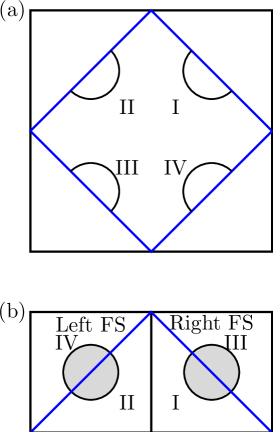
Figure 1: The Brillouin zone and Fermi surface of free holon with $\pi$ flux. The folded MBZ with blue lines as boundary in (a) is equivalent to the rectangular in (b).

Accordingly, all the holon operators can be labeled by the “flavor” index $\alpha=L,R$ distinguishing left and right Dirac zones, so does the Hamiltonian of free holons $\hat{H}^{h}_{0}=\sum_{\alpha=L,R}\hat{H}^{h}_{0,\alpha}$ with

$$\hat{H}^{h}_{0,\alpha} = \sum_{\vec{k}}(t_{\alpha,\vec{k}}\hat{a}^{\dagger}_{\alpha,\vec{k}}\hat{b}_{\alpha,\vec{k}}+h.c.)$$ (22)

$$-\mu(\hat{a}_{\alpha,\vec{k}}^{\dagger}\hat{a}_{\alpha,\vec{k}}+\hat{b}_{\alpha,\vec{k}}^{\dagger}\hat{b}_{\alpha,\vec{k}}),$$

where $t_{R,\vec{k}}\approx 2t(-k_{x}+ik_{y})$ and $t_{L,\vec{k}}\approx 2t(k_{x}+ik_{y})$. In Eq. (22), the momentum $\vec{k}$ only takes values in the range $[-\pi/2,\pi/2]\times[-\pi/2,\pi/2]$, which is one quarter of the original BZ.

Now we consider the holon-holon interactions. As shown in Sec. II.2, the last term in Eq. (10) is repulsive for holons which cannot be the pairing force between holons, and is usually negligible in the low doping limit. Meanwhile, the third term in Eq. (10) implies an effective long-range interaction between the holons mediated by the spin vortices bound to holons, which turns out to be attractive between different Néel sublattices. This leads to the instability of holons towards pair formation and is our key attractive force. Such an effect in the simplest form was first realized by S. TrugmanTrugman (1988) in the early days of High Tc research, who pointed out that putting two holes next to each other on two Néel sublattices would save energy $J$. We include this effect in MFA by introducing a term coming from the average of $z^{\dagger}z$ in  (14) obtaining:

$$J_{\text{eff}}\sum_{i,j}(-1)^{|i|+|j|}\triangle^{-1}(i-j)\hat{h}^{\dagger}_{i}\hat{h}_{i}\hat{h}^{\dagger}_{j}\hat{h}_{j}.$$ (23)

In the static approximation for holons, Eq. (23) describes a 2D lattice Coulomb gas with charges $\pm 1$ depending on the Néel sublattice and coupling constant $J_{\text{eff}}=\tilde{J}\langle z^{\dagger}z\rangle$, where the average $\langle z^{\dagger}z\rangle$ can be estimated from the free spinon spectrum (which will be given in the next section, see Eq. (52) by setting $\Delta_{0}^{s}=0$) with the following result

$$J_{\text{eff}} = \tilde{J}\int d^{2}\vec{q}(q^{2}+m_{s}^{2})^{-1/2}$$ (24)

$$= J(1-2\delta)(\sqrt{\Lambda^{2}+m_{s}^{2}}-m_{s}),$$

where $\Lambda$ is the momentum cutoff for spinon excitations. For 2D Coulomb gases with the above parameters a pairing appears for a temperature $T_{ph}\approx{J_{\text{eff}}}/2\pi$ (a more precise estimation is given later, in fact, $T_{ph}$ is the upper PG crossover temperature determined by $\Delta_{0}^{h}(k_{F})$ of Eq. (36)) which turns out to be inside the SM “phase”. Hence the whole PG “phase” lies below $T_{ph}$. However, we will discuss only the SC arising from the PG phase, anticipating that extrapolation to SM phase will introduce only quantitative changes (actually the role of a next nearest neighbor hopping $t^{\prime}$-term appears relevant in SMgam ). In the large-scale limit the two dimensional Coulomb interaction gives rise to a screening effect, with a screening length $\ell_{s}$ which in the Thomas-Fermi approximation is proportional to $1/\sqrt{\delta}$.Deutsch and Lavaud (1973) In view of the above considerations we approximate the large-scale effective potential in momentum space by

$$V_{\text{eff}}(\vec{p})\approx\frac{J_{\text{eff}}}{p^{2}+\ell_{s}^{-2}}.$$ (25)

The large-scale holon interaction then has the following simplified form

$$H^{h}_{I} \sim -\sum_{\vec{p}_{1}\vec{q}_{1}\vec{p}_{2}\vec{q}_{2}}V_{\text{eff}}(\vec{q}_{1}-\vec{q}_{2})$$ (26)

$$\times\delta(\vec{p}_{1}-\vec{p}_{2}+\vec{q}_{1}-\vec{q}_{2})\hat{a}^{\dagger}_{\vec{p}_{1}}\hat{b}^{\dagger}_{\vec{q}_{1}}\hat{b}_{\vec{q}_{2}}\hat{a}_{\vec{p}_{2}}.$$

Due to the long range tail of vortex-vortex interaction, the pairing strength for large momentum($\vec{q}\sim(\pi,0)$) transfer between different Dirac cones is much smaller than that for small momentum($\vec{q}\sim 0$) transfer. Hence, in the presence of interaction, the left and right flavors of holons can still be decoupled approximately. Considering the BCS approximation, where pairing occurs between holons in states with opposite momentum, one obtains the decoupled Hamiltonians $H^{h}_{I,\alpha}$ for each flavor $\alpha$,

$$\hat{H}^{h}_{I,\alpha}=-\sum_{\vec{p},\vec{q}}V_{\text{eff}}(\vec{p}-\vec{q})\hat{a}^{\dagger}_{\alpha,\vec{p}}\hat{b}^{\dagger}_{\alpha,-\vec{p}}\hat{b}_{\alpha,-\vec{q}}\hat{a}_{\alpha,\vec{q}}.$$ (27)

We shall now focus only on the quasiparticles near the Fermi circles, which allows us to make the following gauge transformations for the holon operators with different flavors separately

$$\hat{a}_{\alpha,\vec{k}}\rightarrow\hat{a}_{\alpha,\vec{k}}e^{i\theta_{\alpha,\vec{k}}/2},\hskip 5.69046pt\hat{b}_{\alpha,\vec{k}}\rightarrow\hat{b}_{\alpha,\vec{k}}e^{-i\theta_{\alpha,\vec{k}}/2},$$ (28)

where the angles $\theta_{\alpha,\vec{k}}$ are chosen to cancel the phase of $t_{\vec{k}}$ so that the kinetic term reads

$$\hat{H}^{h}_{0,\alpha}\approx v_{F}k(\hat{a}^{\dagger}_{\alpha,\vec{k}}\hat{b}_{\alpha,\vec{k}}+h.c.)$$ (29)

with $v_{F}=2t$. Eqs. (27) and  (29) are our basic equations to describe the pairing of holons.

III.2 D-wave Pairing

In this subsection, we show that the $d$-wave pairing symmetry is composed naturally of two $p$-wave pairing within the left and right Dirac cones, an idea first proposed by Sushkov et al.Kuchiev and Sushkov (1993); Flambaum et al. (1994) in a different setting. The corresponding pairing parameter has a form respecting the $C_{4v}$ rotation symmetry,

$$\Delta^{h}_{\alpha,\vec{k}}=\left\{\begin{array}[]{ll}\Delta^{h}(k)\frac{k_{x}-k_{y}}{k},\text{ if }\alpha=R,\\ \Delta^{h}(k)\frac{-k_{x}-k_{y}}{k},\text{ if }\alpha=L,\end{array}\right.$$ (32)

where the momentum $\vec{k}$ is measured from $\vec{Q}_{R,L}$, respectively, and the magnitude of the order parameter is the same for both $R$ and $L$ flavors. Note that we are now working with the rectangular magnetic Brillouin zone (see Fig.1b) and the $p$-wave pairing takes place within the two circular Fermi surfaces. If transformed back to diamond magnetic Brillouin zone as in Fig. 1a, the order parameters in region III and IV change their signs due to the fact that $\hat{b}_{\vec{k}+\vec{\pi}_{\pm}}=-\hat{b}_{\vec{k}}$, which leads to a perfect d-wave pairing in the original Brillouin zone.

Applying the standard BCS treatment we get the following MF Hamiltonian

$$\hat{H}^{h}_{\alpha}=\hat{H}^{h}_{0,\alpha}+\sum_{\vec{k}}(\Delta^{h}_{\alpha,\vec{k}}\hat{a}^{\dagger}_{\alpha,\vec{k}}\hat{b}^{\dagger}_{\alpha,-\vec{k}}+h.c.),$$ (33)

where the order parameter satisfies the gap equations,

$$\Delta^{h}_{\alpha,\vec{k}}=\sum_{\vec{q}}V_{\text{eff}}(\vec{k}-\vec{q})\frac{\Delta_{\alpha,\vec{q}}^{h}}{2\epsilon_{\alpha,\vec{q}}}\tanh\left(\frac{\epsilon_{\alpha,\vec{q}}}{2T}\right).$$ (34)

It turns out that Eq. (33) has two decoupled branches of solutions (see Appendix A for details). One of them with higher energy without FS provides a matrix element suppressing the spectral weight of the original holon field $\hat{h}$ outside the MBZ as in PG.Marchetti et al. (2004a) The other one is responsible for the low energy physics of holon pairing which we will focus on in the following and its spectrum has a simple BCS form

$$\epsilon^{h}_{\vec{k}}=\sqrt{(v_{F}k-\mu)^{2}+|\Delta_{\vec{k}}|^{2}}.$$ (35)

As common for non-weakly coupled attractive Fermi systems, the MF temperature at which $\Delta^{h}$ becomes non-vanishing should be identified with the pairing temperature $T_{ph}$.

For brevity, we consider the $p$-wave order parameter in the right cone, which has the form $\Delta^{h}_{\vec{k}}=\Delta_{0}^{h}(k)(\cos\theta_{\vec{k}}-\sin\theta_{\vec{k}})$. The radial part $\Delta_{0}^{h}(k)$ is decoupled from its angular part approximately (see Appendix A), which is plotted in Fig. 2 for different values of the screening length $\ell_{s}$. We observe that holons near the Fermi surface take part in pairing which results in a peak of $\Delta^{h}(k)$ centered around $k\sim k_{F}$. Actually, the number of holons participating in pairing is determined by the screening length $\ell_{s}$. If we increase $\ell_{s}$, a higher percentage of holons can interact with each others at longer distance, the peak of $\Delta^{h}(k)$ in Fig. 2 becomes higher and wider, that implies a bigger fraction of holons is involved in pairing. A more rigorous treatment would actually involve taking into account self-consistently the UV cutoff and chemical potential change, as discussed e.g. in Refs. Schmitt-Rink et al., 1989; Randeria et al., 1990, but for simplicity we refrain to do that, assuming that our system is sufficiently BCS-like and our treatment catches already the key behavior, as Fig. 2 suggests.

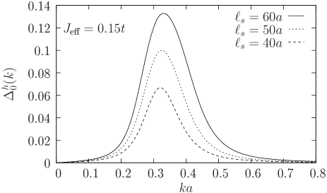
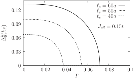
Figure 2: Plots of pairing gap of holon as functions of momentum in the upper panel, and as functions of temperature in the lower panel for different screening length $\ell_{s}$. $\Delta_{0}^{h}$ is plotted in units of $t$. It is seen that the holons near the Fermi surface take part in pairing, leading to a peak of $\Delta(k)$ center around $k\sim k_{F}$.

The maximum value of the order parameter at zero temperature can be taken as the typical energy scale of pairing strength, which is the value of $\Delta_{0}^{h}$ at the Fermi momentum. Though it is difficult to get an analytical solution of $\Delta_{0}^{h}(k_{F})$ from the radial gap equation (see Eq. (85)), one can get an approximate expression for it as a function of the parameters $J_{\text{eff}}$, $k_{F}$ and $\ell_{s}$, which has the following form

$$\Delta^{h}_{0}(k_{F})\approx 0.06J_{\text{eff}}(k_{F}\ell_{s})\exp\left(-\frac{40\mu}{J_{\text{eff}}(k_{F}\ell_{s})^{2}}\right),$$ (36)

being not sensitive to the energy cutoff as long as the screening length $\ell_{s}$ is larger than $1/\Lambda$.

Now we can write down the $d$-wave order parameters near the original four Fermi arcs (see Fig. 1a)

• $\Delta^{h}_{\vec{k}}\approx v_{\Delta}(k_{x}-k_{y})/\sqrt{2}$ in quadrant I,

• $\Delta^{h}_{\vec{k}}\approx v_{\Delta}(-k_{x}-k_{y})/\sqrt{2}$ in quadrant II,

• $\Delta^{h}_{\vec{k}}\approx v_{\Delta}(-k_{x}+k_{y})/\sqrt{2}$ in quadrant III,

• $\Delta^{h}_{\vec{k}}\approx v_{\Delta}(k_{x}+k_{y})/\sqrt{2}$ in quadrant IV,

where $v_{\Delta}\equiv\sqrt{2}\Delta^{h}_{0}(k_{F})/k_{F}$.

So far we discussed the $d$-wave paring symmetry in the momentum space in the long wavelength limit, and now we check that when extrapolating the result to the lattice scale we recover the desired pairing symmetry in real space. Computing the nearest neighbor pairing between site $\vec{x}$ and $\vec{x}+\vec{\delta}$ we get,

$$\langle\hat{b}_{\vec{x}}\hat{a}_{\vec{x}+\vec{\delta}}\rangle\approx\frac{1}{V}\sum_{\vec{k},\alpha}[\langle\hat{b}_{\alpha,-\vec{q}}\hat{a}_{\alpha,\vec{q}}\rangle e^{i\vec{Q}_{\alpha}\cdot\vec{\delta}}]e^{i\vec{k}\cdot\vec{\delta}},$$ (37)

where $V$ is the volume of the system and the summation over $\vec{k}$ is in the range $[-\pi/2,\pi/2]\times[-\pi/2,\pi/2]$. Note that $\langle\hat{b}_{\alpha,-\vec{q}}\hat{a}_{\alpha,\vec{q}}\rangle$ has the same symmetry as $\Delta^{h}_{\alpha,\vec{q}}$ (see Eq. (A)), then by using Eq. (32), one can easily prove $\langle\hat{b}_{\vec{x}}\hat{a}_{\vec{x}+\vec{\delta}}\rangle=\langle\hat{b}_{\vec{x}}\hat{a}_{\vec{x}-\vec{\delta}}\rangle$ and $\langle\hat{b}_{\vec{x}}\hat{a}_{\vec{x}+\vec{e}_{1}}\rangle=-\langle\hat{b}_{\vec{x}}\hat{a}_{\vec{x}+\vec{e}_{2}}\rangle$, which are the typical features of d-wave order parameters in real space.

III.3 Nodal approximation and Gauge Invariance

In the BCS approximation discussed in the previous subsection the holon is gapless only at the 4 nodal points of $\Delta^{h}_{\vec{k}}$. However, in a large-scale gauge-invariant treatment whereas one can keep the modulus of the order parameter $\Delta^{h}$ as in BCS, we must include its spatially dependent phase, which we denote by $\phi^{h}(x)$. (A precise procedure to go from the lattice to the continuum phase field is discussed in Ref. Tešanović, 2008.) The effects of $\phi^{h}(x)$ on holons is non-trivial and will be discussed in detail in Ref. gam, . However, to derive our basic RVB gap equation in the next section it turns out that we can assume consistently that $\phi^{h}(x)$ doesn’t break the nodal structure. In fact the nodal structure appears if we neglect the phase fluctuations, so that the holon pairs are assumed condensed. According to Refs. Nozieres and Schmitt-Rink, 1985; Botelho and Sá de Melo, 2006; Tempere et al., 2009 this is the correct procedure to deal with the gap equation for the modulus of the order parameter. However, if holon pairs are only formed but not yet condensed, it is incorrect to identify $\Delta^{h}$ as the gap for holons (see Ref. gam, ).

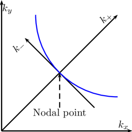
Figure 3: The coordinate system $(k_{+},k_{-})$ taken in the nodal approximation. This is for the first quadrant.

In this subsection we utilize the Peierls substitution to take the gauge fields back into account around the nodal points, in agreement with the above remarks. In the nodal approximation the momenta are expanded around the nodes in the four quadrants of the MBZ. In Fig. 3, we plot the nodal coordinate system in the 1st quadrant, where

$$k_{x}=\frac{k_{+}+k_{-}}{\sqrt{2}},\hskip 5.69046ptk_{y}=\frac{k_{+}-k_{-}}{\sqrt{2}}.$$ (38)

In terms of $k_{+}$ and $k_{-}$, using the the gap dependence on momentum $\vec{k}$ obtained in the last subsection, the energy spectrum around the node of the 1st quadrant is simply $\pm\sqrt{v_{F}^{2}k_{+}^{2}+v_{\Delta}^{2}k^{2}_{-}}$, which arises from the nodal Hamiltonian in the 1st quadrant

$$\mathcal{H}^{h}_{\text{1st nodal}}=v_{F}k_{+}\sigma_{z}+v_{\Delta}k_{-}\sigma_{y},$$ (39)

which reproduces the spectrum of the gapless nodal excitation. Therefore, adding also the contribution of the phase $\phi^{h}(x)$ of the order parameter, a large-scale h/s gauge invariant Hamiltonian in real space reads

$$\mathcal{H}^{h}_{\text{1st}}=\begin{pmatrix}-i\partial_{+}-A_{+}+A_{0}&-e^{i\phi^{h}}\partial_{-}\\ e^{-i\phi^{h}}\partial_{-}&i\partial_{+}-A_{+}-A_{0}\end{pmatrix},$$ (40)

where the emergent gauge field $A_{+}$ and $A_{0}$(see Eq. (18)) is reinserted, and the parameters $v_{F}$ and $v_{\Delta}$ are omitted for the sake of simplicity. There is an obvious U(1) redundancy of this Hamiltonian. Let us denote the nodal Dirac quasi-particles field by $\chi_{\alpha}(x)$. The $h/s$ gauge transformation $\chi\rightarrow\chi e^{i\Lambda},\phi^{h}\rightarrow\phi^{h}+2\Lambda,A_{\mu}\rightarrow A_{\mu}+\partial_{\mu}\Lambda$ leaves Eq. (40) invariant provided that $\Lambda$ is time independent. We then make the field redefinition from $\chi_{\alpha}$ to $\tilde{\chi}_{\alpha}$ as $\tilde{\chi}_{1}=\chi_{1}e^{i\phi^{h}/2}$ and $\tilde{\chi}_{2}=\chi_{2}e^{-i\phi^{h}/2}$, so that the nodal field becomes neutral under h/s gauge transformations, a ‘nodon’.Senthil and Fisher (2001) The above redefinition leads to a more convenient form of the nodal Hamiltonian:

$$\mathcal{H}_{\text{1st}} = \begin{pmatrix}-i\partial_{+}-a_{+}+a_{0}&-\partial_{-}\\ \partial_{-}&i\partial_{+}-a_{+}-a_{0}\end{pmatrix}$$ (41)

$$= -a_{+}+(-i\partial_{+}+a_{0})\sigma_{3}-i\partial_{-}\sigma_{2},$$

where the h/s gauge invariant field $a_{\mu}=A_{\mu}-\frac{1}{2}\partial_{\mu}\phi^{h}$ is introduced.

Rotating the coordinate by $\pi/2$ successively, one may get the nodal Hamiltonian in the other three quadrants.

III.4 Effective Action of $a_{\mu}$

In this subsection, we turn to the path-integral formalism and derive an effective action (needed to discuss RVB gap equation) for $a_{\mu}$ in the nodal approximation by integrating out the holon fields. In the 1st quadrant, the effective Lagrangian in the Euclidean space for nodal quasi-particles is given by:

$$\mathscr{L}^{\text{1st}}=\bar{\chi}(x)[\gamma^{\mu}(\partial_{\mu}-ib^{\text{1st}}_{\mu})]\chi(x),$$ (42)

where $\gamma^{\mu}=\{\sigma_{x},-\sigma_{y},\sigma_{z}\}$, $\partial_{\mu}=\{\partial_{0},\partial_{+},\partial_{-}\}$ and $b^{\text{1st}}_{\mu}=\{-ia_{+},ia_{0},0\}$. The effective action for $b^{\mu}$ (at $T=0$) is defined as

$$S^{1st}_{\text{eff}}[a^{\mu}]=-\ln\det[\gamma^{\mu}(\partial_{\mu}-ib^{\text{1st}}_{\mu})]\approx$$

$$-\frac{1}{2}\int d^{2}k\int d\omega[b^{\text{1st}}_{\mu}\Pi^{\text{1st}}_{\mu\nu}b^{\text{1st}}_{\nu}](\vec{k},\omega).$$ (43)

By adapting the calculations of Ref. Sharapov et al., 2001, the leading terms of the bubbles for small $\omega,|\vec{k}|,\omega/|\vec{k}|$ behave like

$$\Pi^{\text{1st}}_{00}\sim c_{1}|\vec{k}|,\hskip 5.69046pt\Pi^{\text{1st}}_{++}\sim c_{2},\hskip 5.69046pt\Pi^{\text{1st}}_{0+}\sim 0.$$ (44)

The effective action in the other three quadrants is similar to that in Eqs. (III.4) and (44). For example, the 3rd quadrant can be obtained by rotating the coordinate by $\pi$, therefore by changing $a_{\pm}\rightarrow-a_{\pm}$ and $\partial_{\pm}\rightarrow-\partial_{\pm}$, we can obtain the corresponding bubble $\Pi_{\mu\nu}$ and gauge field $b_{\mu}$. Note that the coordinate transformation does not involve the time axis. Then we have

• $\Pi_{\mu\mu}^{\text{3rd}}=\Pi^{\text{1st}}_{\mu\mu}$, if $\mu=0,1,2$,

• $b^{\text{3rd}}_{\mu}=\{ia_{+},ia_{0},0\}.$

Similar procedure can be applied to the 2nd and 4th quadrants.

After summing over all four quadrants, in the quadratic approximation, we have the effective action

$${S}^{h}_{\text{eff}}[a_{\mu}] = \int d^{2}k\int d\omega\sum_{i=+,-}$$ (45)

$$[a_{i}\Pi_{00}a_{i}+a_{0}\Pi_{ii}a_{0}-2a_{0}\Pi_{0i}a_{i}](\vec{k},\omega).$$

Using Eq. (44) and its analogues one sees that Eq. (45) is a variant of the effective action for QED₃.

IV Spinon RVB Pairing

IV.1 Mean Field Lagrangian with Spinon Pairing

In this subsection we derive the mean field Lagrangian for spinon pairing in the presence of holon pairs.

In the PG region, the spinon part in the $t-J$ model can be described by the massive sigma model in CP¹ form Eq. (17), and the four fermion interaction term $\sim J(\hat{h}^{\dagger}_{i}\hat{h}^{\dagger}_{j}\hat{\Delta}^{s\dagger}_{ij})(\hat{h}_{j}\hat{h}_{i}\hat{\Delta}^{s}_{ij})$ (see the last term in Eq. (10)), is simply neglected for small doping $\delta$ in considering the normal state, because it is proportional to $\delta^{2}$. Note this interaction term is positive (for $J>0$), hence repulsive due to the semionic mean field approach, contrary to the usual fermionic case. However, once the holon pairing is stabilized, the gauge interaction between holon and spinon, overcoming the above repulsion forces the spinons to form singlet-RVB pairs and the above term becomes relevant. To investigate the spinon pairing, one can apply a Hubbard-Stratonovich transformation to the four fermion interaction term, obtaining

$$\sum_{\langle ij\rangle}-\frac{2|\Delta^{s}_{ij}|^{2}}{J\tau^{2}}+\Delta^{s*}_{ij}\epsilon^{\alpha\beta}z_{i\alpha}z_{j\beta}+h.c.,$$ (46)

where $\tau\equiv|\langle\hat{h}_{i}\hat{h}_{j}\rangle|$ and in MFA

$$\Delta^{s}_{ij}=\frac{J}{2}\tau^{2}\langle\epsilon^{\alpha\beta}\hat{z}_{i\alpha}\hat{z}_{j\beta}\rangle=\frac{J}{2}\tau^{2}\langle\hat{\Delta}^{s}_{ij}\rangle.$$ (47)

In the continuum limit we get the Lagrangian for spinon with a singlet spinon pairing

$$\mathscr{L}_{s} = \sum_{\mu=0,1,2}z^{*}_{\alpha}[(\partial_{\mu}-iA_{\mu})^{2}+m^{2}_{s}]z_{\alpha}$$ (48)

$$+\sum_{i=1,2}\Delta^{s*}_{i}(\vec{x})\epsilon^{\alpha\beta}z_{\alpha}(\vec{x})\partial_{i}z_{\beta}(\vec{x})+h.c.,$$

where the index $i$ in $\Delta^{s*}$ labels the spatial directions and we set $g$ and $v_{s}$ to 1 for convenience. (The spatial derivative term in the square brackets has an implicit ‘-’ sign, see Eq. (17).) As for the holon case, one can rewrite approximately the spinon pairing as $\Delta_{i}^{s}(\vec{x})=\Delta_{i,0}e^{i\phi^{s}(\vec{x})}$ where $\phi^{s}$ is the phase of the spinon pairing amplitude. The Lagrangian Eq. (48) is invariant under the h/s gauge transformation $z_{\alpha}\rightarrow z_{\alpha}e^{i\Lambda}$, $A_{\mu}\rightarrow A_{\mu}+\partial_{\mu}\Lambda$ and $\phi^{s}\rightarrow\phi^{s}+2\Lambda$. It is not convenient to deal with the off-diagonal terms in the Lagrangian $\mathcal{L}_{s}$, hence we transform the spinon field from $z_{\alpha}$ to $\tilde{z}_{\alpha}$ as $\tilde{z}_{1}=z_{1}e^{i\phi^{s}/2}$,$\tilde{z}_{2}=z_{2}^{*}e^{-i\phi^{s}/2}$ so that the spinon field becomes neutral under h/s gauge transformations. In terms of the new fields $\tilde{z}_{\alpha}$, the spinon Lagrangian can be written in a diagonal form $\mathscr{L}_{s}(x)=\tilde{z}^{\dagger}(x)\Gamma_{s}(x)\tilde{z}(x)$ where the $2\times 2$ kernel $\Gamma_{s}$ reads (with $\Delta^{s}_{0,0}=0$)

$$\Gamma_{s}=\sum_{\mu=0,1,2}-[\partial_{\mu}-i(a_{\mu}+\frac{1}{2}\partial_{\mu}\phi)\sigma_{z}-i\text{Im}(\Delta^{s}_{\mu,0})\sigma_{x}-i\text{Re}(\Delta^{s}_{\mu,0})\sigma_{y}]^{2}+m^{2}_{s}-|\Delta^{s}_{\mu,0}|^{2},$$ (49)

with $\phi=\phi^{h}-\phi^{s}$ and $a_{\mu}=A_{\mu}-\frac{1}{2}\partial_{\mu}\phi^{h}$, both of which are h/s gauge invariant. The gradient of the $\phi$ field actually describes the potential of standard magnetic vortices, since from Eqs. (20) and  (47) $\phi$ is the phase of the condensate of hole-pairs.

By neglecting the gauge fields, one can work out the spinon spectrum, which can be obtained from the zeros of the determinant of the kernel $\Gamma_{s}$ in the momentum space:

$$(-\omega^{2}+k^{2}+m^{2}_{s})^{2}-4\sum_{i,j=1,2}\Delta^{s}_{i,0}\Delta^{s*}_{j,0}k_{i}k_{j}=0.$$ (50)

We assume the rotational invariance for the spinon spectrum, which requires

$$\Delta^{s}_{i,0}\Delta^{s*}_{j,0}+\Delta^{s*}_{i,0}\Delta^{s}_{j,0}=2\delta_{ij}|\Delta^{s}_{i,0}|^{2}.$$ (51)

We can take $\Delta^{s}_{1,0}=\Delta_{0}^{s}$ and $\Delta^{s}_{2,0}=\pm i\Delta_{0}^{s}$, where $\Delta^{s}_{0}$ can be a priori any complex number, and both plus and minus signs are allowed for $\Delta^{s}_{2,0}$. Looking at the hole-pair order parameter Eq. (20), we see, however, that for consistency we have to choose the constant phases of $\Delta^{s}_{0}$ equal to $-\bar{B}_{ij}$ to ensure the correct symmetry, being the hole-pair $d$-wave. From Eq. (50) we obtain the spectrum for spinon: it has two (positive) branches

$$E_{\pm}(\vec{k})=\sqrt{\vec{k}^{2}+m^{2}_{s}\pm 2\Delta_{0}^{s}|\vec{k}|}$$ (52)

which are plotted in Fig. 4.

Figure 4: The spinon spectrum for $\delta=0.1$.

The positive branches of the dispersion are similar to those found in a plasma of relativistic fermions,Weldon (1989) which suggests the following interpretation: if $|\Delta^{s}|\neq 0$ the spinon system contains a gas of RVB spinon pairs, an analogue of Coulomb neutral pairs in the relativistic plasma, either in the plasma phase if $\langle\Delta^{s}\rangle=0$, or in a condensate if $\langle\Delta^{s}\rangle\neq 0$. For a finite density of spinon pairs there are two (positive energy) excitations, with different energies, but the same spin and momenta. They are given, e.g., by creating a spinon up and by destructing a spinon down in one of the RVB pairs. Notice that the minimum at $\tilde{J}|\vec{k}|=|\Delta^{s}|$ in the lower branch is similar to the roton minimum in superfluid helium and has an energy lower than $m_{s}$; it implies a backflow of the gas of spinon-pairs dressing the “bare spinon”. Hence RVB condensation would lower the spinon kinetic energy. However, to make it occur one needs the gauge contribution to overcome the spinon repulsion generated by the Heisenberg term.

IV.2 Effective action of Gauge fields

In this subsection, we derive the low-energy effective action of $a_{\mu}$ and $\phi$ by integrating over the spinon fields. For this purpose we introduce a fictitious SU(2) gauge fields $Y_{\mu}$ as follows:

$$Y_{\mu}=\sum_{a=x,y,z}Y^{a}_{\mu}\frac{\sigma_{a}}{2}$$ (53)

with

$$Y^{a}_{\mu}=2\begin{pmatrix}0&0&a_{0}+\partial_{0}\phi\\ \text{Im}(\Delta^{s}_{1,0})&\text{Re}(\Delta^{s}_{1,0})&a_{1}+\frac{1}{2}\partial_{1}\phi\\ \text{Im}(\Delta^{s}_{2,0})&\text{Re}(\Delta^{s}_{2,0})&a_{2}+\frac{1}{2}\partial_{2}\phi\end{pmatrix}.$$ (54)

Then the kernel $\Gamma_{s}$ (see Eq. (49)) can be written in a compact form

$$\Gamma_{s}=\sum_{\mu}(\partial_{\mu}-iY^{a}_{\mu}\frac{\sigma^{a}}{2})^{2}+M^{2},$$ (55)

where we introduce the notation

$$M=\sqrt{m^{2}_{s}-2|\Delta^{s}_{0}|^{2}}$$ (56)

for convenience. After integrating over the spinon fields $z_{\alpha}$, one obtains the effective action for $a_{\mu}$ and $\partial_{\mu}\phi$,

$$S_{\text{eff}}^{s}[\partial_{\mu}\phi,a_{\mu},\Delta^{s}_{0}]=\ln\det(\Gamma_{s})-\frac{2|\Delta_{0}^{s}|^{2}}{J\tau^{2}},$$ (57)

where the constant term comes from the Hubbard-Stratonovich transformation. Since Eq.  (55) is formally describing a relativistic 2-component boson of mass $M$ minimally coupled to the SU(2) gauge field $Y^{a}_{\mu}$, the leading gauge invariant term is the Yang-Mills Lagrangian, i.e., the traced square ($\sum_{\mu\nu}Y_{\mu\nu}^{a}Y_{\mu\nu}^{a}$) of the field strength $Y_{\mu\nu}$

$$Y_{\mu\nu}=\frac{\sigma^{c}}{2}[\partial_{\mu}Y_{\nu}^{c}-\partial_{\nu}Y^{c}_{\mu}+\epsilon^{abc}Y^{a}_{\mu}Y^{b}_{\nu}]$$ (58)

and one easily computes, with $i=1,2$:

$$Y_{0i}^{x}=-(a_{0}+\partial_{0}\phi)\mbox{Re}(\Delta_{i0}^{s}),$$

$$Y_{12}^{x}=\mbox{Re}(\Delta^{s}_{10})(a_{2}+\partial_{2}\phi)-\mbox{Re}(\Delta^{s}_{20})(a_{1}+\partial_{1}\phi),$$

$$Y_{0i}^{y}=(a_{0}+\partial_{0}\phi)\mbox{Im}(\Delta_{i0}^{s}),$$

$$Y_{12}^{y}=\mbox{Im}(\Delta^{s}_{20})(a_{1}+\partial_{1}\phi)-\mbox{Im}(\Delta^{s}_{10})(a_{2}+\partial_{2}\phi),$$

$$y_{0i}^{z}=\partial_{0}(a_{i}+\partial_{i}\phi)-\partial_{i}(a_{0}+\partial_{0}\phi),$$

$$y_{12}^{z}=\partial_{1}(a_{2}+\partial_{2}\phi)-\partial_{2}(a_{1}+\partial_{1}\phi),$$

$$+\mbox{Im}(\Delta^{s}_{10})\mbox{Re}(\Delta^{s}_{20})-\mbox{Im}(\Delta^{s}_{20})\mbox{Re}(\Delta^{s}_{10}).$$

Besides the Yang-Mills action there are also gauge non-invariant terms which arise from the ultra-violet divergences of the continuous model and must be included since the $x,y$ components of $Y^{a}_{\mu}$ are actually constant. For the 0th and 2nd order terms in $a_{\mu}$ and $\phi$ we finally get

$$S^{s,0}_{\text{eff}}=-\frac{2|\Delta_{0}^{s}|^{2}}{{J}\tau^{2}}+\sum_{\omega,\vec{k}}\ln[(\omega^{2}+E^{2}_{-}(\vec{k}))(\omega^{2}+E^{2}_{+}(\vec{k}))],$$

$$S^{s,2}_{\text{eff}}=\frac{1}{6\pi M}\{[\partial_{\mu}a_{\nu}-\partial_{\nu}a_{\mu}]^{2}$$

$$+|\Delta^{s}_{0}|^{2}[2(a_{0}+\frac{1}{2}\partial_{0}\phi)^{2}+(\vec{a}+\frac{1}{2}\vec{\nabla}\phi)^{2}]\},$$ (59)

where a surface term ($\sim\partial_{1}a_{2}-\partial_{2}a_{1}$) has been discarded. For $|\Delta^{s}_{0}|\neq 0$, $S^{s,2}_{\text{eff}}$ is the action of a gauged XY or Stueckelberg model and the term in the last square bracket is the celebrated Anderson-Higgs mass term.

IV.3 Gap equation of spinon pairing

The gap equation is determined by the saddle point of $S_{\text{eff}}^{s}[a,\Delta_{0}^{s}]=S^{s,0}_{\text{eff}}[\Delta_{0}^{s}]+S^{s,2}_{\text{eff}}[a,\Delta_{0}^{s}]+S^{h}_{\text{eff}}[a]$ with respect to $\Delta_{0}^{s}$. Note that since the interaction between spinons is repulsive, it is crucial to take the gauge fluctuation $S^{s,2}_{\text{eff}}$ into account, unlike in the traditional BCS theory, where the electron interaction is attractive. To establish the gap equation for the modulus of the order parameter, we assume, as discussed e.g. in Refs. Nozieres and Schmitt-Rink, 1985; Botelho and Sá de Melo, 2006; Tempere et al., 2009 for fermions, that one should neglect the phase ($\phi$) fluctuations. Let us also neglect for simplicity at first the holon contribution $S^{h}_{\text{eff}}$, then the resulting gauge partition function, denoted by $Z_{g}$, is given by:

$$Z_{g} = \int D[a_{\mu}]e^{-\int d^{3}x\mathscr{L}_{g}[a_{\mu}]},$$

$$\mathscr{L}_{g} = \frac{1}{3\pi M}\left[a_{\mu}(-\partial^{2}g^{\mu\nu}+\partial^{\mu}\partial^{\nu}+|\Delta_{0}^{s}|^{2}\lambda^{\mu\nu})a_{\nu}\right],$$ (60)

where $g^{\mu\nu}=\text{diag}(1,1,1)$ and $\lambda^{\mu\nu}=\text{diag}(1,1/2,1/2)$ are $3\times 3$ diagonal matrices and a cutoff $\Lambda$ in both momenta and energy is understood. The equation of motion of gauge field $a_{\mu}$ reads

$$-\partial^{2}a_{\mu}+\partial^{\mu}(\partial_{\nu}a_{\nu})+\lambda^{\mu\nu}a_{\nu}=0,$$ (61)

which implies that (without source) $a_{\mu}$ satisfies the equation

$$\lambda^{\mu\nu}\partial_{\mu}a_{\nu}=0.$$ (62)

Eq. (62) is a constraint, meaning that the massive vector bosons in two dimensions have two (physical) polarization modes. Therefore, the calculation of the partition function of the vector boson is not as trivial as integrating over $a_{\mu}$ directly, in fact one must take care to count only the physical degrees of freedom. The details of the evaluation of $Z_{g}$ is given in Appendix B. Here we only give the final result

$$Z_{g} = \prod_{\omega,\vec{k}}\left[(3\pi M)^{\frac{3}{2}}\left(\omega^{2}+\frac{|\Delta_{0}^{s}|^{2}}{2}+\frac{\vec{k}^{2}}{2}\right)^{-\frac{1}{2}}\right.$$ (63)

$$\hskip 28.45274pt\left.\times\left(\omega^{2}+\frac{|\Delta_{0}^{s}|^{2}}{2}+{\vec{k}^{2}}\right)^{-\frac{1}{2}}\right].$$

The first factor in r.h.s. of Eq. (63) contributes a constant term to the free energy which is neglected in the standard cases. However, in the present case it contains the spinon order parameter $\Delta_{0}^{s}$, which can affect the total energy as $\Delta_{0}^{s}$ varies, hence should be kept. Actually, $3\pi M$ is the renormalization factor of the amplitude of the gauge action, which can be absorbed into $a_{\mu}$ by rescaling $a_{\mu}\rightarrow\sqrt{3\pi M}a_{\mu}$ with a Jacobian left for the measure $D[a_{\mu}]$ in the energy-momentum space

$$D[a_{\mu}]\rightarrow\prod_{\omega,\vec{k}}(3\pi M)^{\frac{3}{2}}D[a_{\mu}],$$ (64)

where the power index $3/2$ is due to the fact that $a_{\mu}$ is a three-dimensional vector.

In fact in the spinon gap equation the term $3\pi M$ already balances the repulsive interaction. The contributions of the spectrum of gauge quasiparticles, i.e., the second and third terms in Eq. (63), do not change the spinon gap equation qualitatively. Therefore, for simplicity we focus only on the $M$-term, and the free energy including the contribution from the h/s gauge fluctuation reads

$$\frac{1}{V}F_{g}[\Delta_{0}^{s}]$$ (65)

$$\approx \frac{1}{\beta V}\sum_{\omega,\vec{k}}\ln[(\omega^{2}+E^{2}_{-}(\vec{k}))(\omega^{2}+E^{2}_{+}(\vec{k}))]$$

$$-\frac{3\Lambda^{3}}{4}\left[\ln m_{s}^{2}-\frac{2|\Delta_{0}^{s}|^{2}}{m_{s}^{2}}\right]-\Lambda^{2}\frac{|\Delta_{0}^{s}|^{2}}{J\tau^{2}}.$$

It is straightforward to obtain the gap equation by taking derivative of $F_{g}$ with respect to $|\Delta_{0}^{s}|^{2}$:

$$0 = \frac{3\Lambda^{3}}{2m^{2}_{s}}-\frac{\Lambda^{2}}{J\tau^{2}}$$ (66)

$$-\frac{1}{2|\Delta_{0}^{s}|V}\sum_{\vec{k}}\left[\frac{k}{E_{-}\tanh\frac{E_{-}}{2T}}-\frac{k}{E_{+}\tanh\frac{E_{+}}{2T}}\right].$$

The first term originates from the gauge action due to the lowering of the spinon mass ($m_{s}\rightarrow(m_{s}^{2}-|\Delta^{s}|^{2})^{1/2}$), while the second term comes from the original repulsive Heisenberg term and the last two terms are due to the spinon excitations. The first term in r.h.s. of Eq. (66) is crucial, without which the gap equation has no solution, since the last term is negative. In Eq. (66) only the value of $\tau$ is unknown, i.e., the nearest neighbor holon pairing strength, which is a very short range correlation and may not be accurate if being calculated via the long wavelength pairing $\Delta_{\vec{k}}^{h}$ in momentum space. However, we have already seen that extrapolating $\Delta_{\vec{k}}^{h}$ to lattice scale, one gets the correct symmetry in real space. Hence we take $\Delta^{h}_{0}(k_{F})$ as the value of $\tau$ up to a scale factor. Let us briefly comment on the relation of our RVB gap equation Eq. (66) with that of the slave boson approach. Whereas in the slave-boson approach the RVB pairs are made of fermions and the Heisenberg term is attractive, so the pair-formation is BCS-like, in our approach the RVB pairs are made of bosons, and the Heisenberg term is repulsive, so the pair formation arises from the decrease in the free energy of spinons, via the lowering of their mass gap, induced by holon-pairing through the gauge field.

So far we have not considered the vector boson quasiparticles, whose spectrum has two branches as derived from Eq. (63),

$$E^{(1)}_{g}(\vec{k})=\sqrt{k^{2}+\frac{|\Delta_{0}^{s}|^{2}}{2}},\hskip 5.69046ptE^{(2)}_{g}(\vec{k})=\sqrt{\frac{k^{2}}{2}+\frac{|\Delta_{0}^{s}|^{2}}{2}}$$ (67)

and contributes to the gap equation with the following term

$$\sim\frac{1}{2V}\sum_{\vec{k},n=1,2}\frac{1}{E^{(n)}_{g}\tanh\frac{E^{(n)}_{g}}{2T}}.$$ (68)

This contribution is positive and in balancing the gap equation Eq. (66) plays a role similar to the $M$-term, that turns out to be dominant. It is interesting to note that Eq. (68) is well defined in the gapped region $\Delta_{0}^{s}\neq 0$, and if $\Delta_{0}^{s}=0$, it is proportional $\sim T\ln L$ which is divergent unless $T=0$ if the typical length of the sample $L$ goes to infinity. Such an infared divergence seems to imply a first order phase transition when spinons begin to pair. However, this is not the case. In fact, when we take into account the contribution of holons $S^{h}_{\text{eff}}$ to the action of gauge field (see Eq. (45)), the dispersions  (66) become (see Appendix B):

$$E^{(1)}_{g}(\vec{k})=\sqrt{k^{2}+f(\vec{k})+\frac{|\Delta_{0}^{s}|^{2}}{2}},$$

$$E^{(2)}_{g}(\vec{k})=\sqrt{\left(\frac{|\Delta_{0}^{s}|^{2}}{2}+f(\vec{k})\right)\left(1+\frac{\vec{k}^{2}}{|\Delta_{0}^{s}|^{2}+\tilde{c}_{2}}\right)},$$ (69)

where $\tilde{c}_{2}=3\pi Mc_{2}$ and $f(\vec{k})=3\pi Mc_{1}\sqrt{v_{F}^{2}k_{+}^{2}+v_{\Delta}^{2}k_{-}^{2}}$, and the divergence disappears.

In the low doping limit at $T=0$, expanding the last terms in the r.h.s. of Eq. (66) we get

$$|\Delta_{0}^{s}|\approx\frac{\Lambda^{3/2}}{m_{s}^{1/2}}\sqrt{1-\frac{m_{s}^{2}}{J\tau^{2}}}.$$ (70)

As the doping $\delta$ is decreased, $\tau$ goes to zero faster than $m_{s}$, because the spinon mass $m_{s}^{2}\sim|\delta\ln\delta|$ and $\tau^{2}\sim\delta e^{-\text{const.}}$(see Eq. (36)), which implies that $|\Delta_{0}^{s}|$ has no nonzero solution for sufficiently small doping. In other words, there is a critical doping $\delta_{c}$ at zero temperature, below which spinon pairing $\Delta_{0}^{s}$ must vanish. As the non-vanishing of $\Delta_{0}^{s}$ is a pre-condition for SC, this implies a critical doping for SC at $T=0$. On the other hand, at the qualitative level, due to the cancellation of $\delta$ between $m_{s}^{2}$ and $\tau^{2}$, if $\tau$ ( i.e. the holon-pairs density) is sufficiently large Eq. (70) does have a solution, because the remaining $|\ln\delta|$ is a decreasing function. Notice again the crucial role of this logarithm, coming from the long-range tail of spin-vortices.

At finite temperatures, we need to solve Eq. (66) numerically. The crossover temperature at which in mean field approximation $\Delta_{0}^{s}$ becomes non-vanishing is denoted by $T_{ps}$ (not yet the SC $T_{c}$) and is related to the formation of a finite density of RVB spinon pairs. From Eq. (36) we see that to have solution for the gap equation we need $\tau=\langle h_{i}h_{j}\rangle\sim\Delta_{0}^{h}\neq 0$, consistently with the physical mechanism proposed, hence $T_{ph}>T_{ps}$ and when the spinon RVB pairs are formed together with the already formed holon pairs, producing a finite density of preformed hole pairs. Due to the $\phi$ phase fluctuations, however, although the modulus of the SC order parameter $\Delta^{c}\sim\Delta^{s}/\Delta^{h}$ of  (20) is non-vanishing, if the hole pairs are not condensed one cannot interpret it as the hole gap. The temperature dependence of $\Delta_{s}$ is presented in Fig.  5b. One can see that, although near $T_{ps}$ the behavior is the typical square root of mean-field, at low $T$ it is definitely not BCS-like, never approaching a constant.

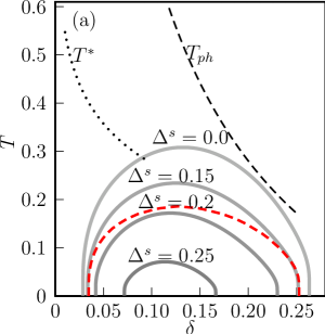
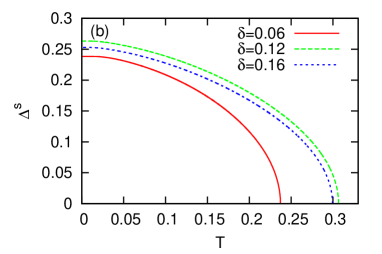
Figure 5: (Color online) (a) is the $T-\delta$ phase diagram of the mean field gap equation of spinon for different values of MF spinon pairing $\Delta^{s}$ (gray lines) which could be compared with different levels of the Nernst signalWang et al. (2002, 2006); $\Delta^{s}=0$ is $T_{ps}$. (The curves at high dopings are not quantitatively reliable as they do not take into account the crossover to the “strange metal”). The dashed line is $T_{ph}$, the “upper PG crossover temperature”. The dotted line is the crossover temperature between the pseudogap and strange metal phases, $T^{*}$. (b) is the $\Delta^{s}$ as a function of temperature for fixed dopings. The temperature and $\Delta^{s}$ are in units of $J$.

V Superconductivity

Now we are ready to finally discuss the true SC transition.

V.1 Nernst crossover

In this subsection we first consider the physical effects due to a finite density of hole pairs before their condensation.

The gauged XY or Stueckelberg model of Eq. (IV.2) is well known to have in the lattice two phases (see Ref. Seiler, 1982 for a rigorous discussion, while Ref. Kleinert, 1989 for a numerical analysis): Coulomb and Higgs. If the coefficient, $\sim|\Delta_{0}^{s}|^{2}$ of the Anderson-Higgs mass term for $a$ is sufficiently small, the phase field $\phi$ fluctuates so strongly that it does not produce a mass gap for $a_{\mu}$ and $\langle e^{i\phi}\rangle=0$ in the Coulomb gauge (a gauge-fixing is necessary due to the Elitzur theoremElitzur (1975)). This is the Coulomb phase, where a plasma of magnetic vortices-antivortices appears. In the presence of a temperature gradient a perpendicular external magnetic field induces an unbalance between vortices and antivortices, giving rise to a Nernst signal, even if the hole-pairs are not condensed yet. Therefore we conjecture that this phase of the model corresponds to the region in the phase diagram of underdoped cuprates characterized by a non-SC Nernst signal and a comparison between the experimental phase diagram in Refs. Wang et al., 2002, 2006 and the one derived in our model, supports this idea. The result is shown in Fig. 5, where the thick lines are equal-$\Delta_{0}^{s}$ lines. One expects that the level of $\Delta_{0}^{s}$ is roughly proportional to the intensity of the Nernst signal and a comparison of the figure with the experimental dataWang et al. (2002, 2006) shows a qualitative agreement for the $\delta-T$ dependence. Note that the Nernst data are strongly supported by the measured magnetic-field induced diamagnetic signal,diam as well as by STM visualized pair formationyazdani and quasi-particle fingerprint.davis The $T_{ph}$ line in the figure is the upper pseudo-gap crossover temperature determined by $\Delta_{0}^{h}(k_{F})$ of Eq. (36), hence it does not take into account the transition to the SM phase, therefore can only be taken as a qualitative trend. At extremely low doping ($\delta\lesssim 0.03$) the lines are not reliable because the quenched approximation for vortices used in our approach is not valid for too low vortex density.

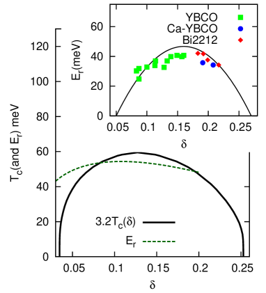
Figure 6: (Color online) The energy of the magnetic resonance $E_{r}$ estimated by $2m_{s}J$ for different dopings, compared with the scaled critical temperature $3.2T_{c}$. To compare with experiments we take $J=100meV$. The inset is the experimental results taken from Ref. Yu et al., 2009, where the black solid line is a parabolic approximation to $T_{c}$ rescaled by 5.8.

V.2 The superconducting transition

Now we consider the true SC transition. For a sufficiently large coefficient $|\Delta^{s}|^{2}$, the gauged XY or Stueckelberg model of Eq. (IV.2) is in the broken symmetry phase: the fluctuations of $\phi$ are exponentially suppressed and $\langle e^{i\phi}\rangle\neq 0$ at $T=0$ or there is a quasi-condensation (power-law-decaying order parameter) at $T>0$; accordingly magnetic vortex-antivortex pairs become small and dilute, so the gauge field is gapped. At the same time the holon, and hence the hole, acquires the nodal gap, i.e. the gap outside the nodes. In fact, one can prove that, due to the fluctuations of the field $\phi^{h}$, in our approach a gapless gauge field is inconsistent with the coherence of holon pairs in PG, i.e., coherent holon pairs cannot coexist with incoherent spinon pairs, as sketched in Appendix C. On the other hand, due to the QED-like structure of holons-gauge action, the gauge field cannot be gapped (in all components) by condensation of holon pairs alone as shown by Eq. (44); only the condensation of RVB spinon pairs at the same time can open a gap to the gauge fluctuations and then the nodal hole gap. Thus as soon as $e^{i\phi^{h}}$ (quasi-)condenses, the same occurs to $\langle h_{i}h_{j}\rangle$, so that SC emerges, since from Eqs. (47) and  (IV.2) the SC order parameter is $\Delta^{c}\sim\Delta^{s}/\langle h_{i}h_{j}\rangle\sim(\Delta^{s}_{0}/\Delta^{h}_{0})e^{i\phi}$ and now its modulus and the expectation of its phase are nonzero (at $T=0$, or power-law decaying at $T>0$). It follows that $T_{c}<T_{ps}$.

According to the above considerations, if we assume that the holon contribution to the gauge field is subdominant, as expected, the SC transition from the PG phase should occur roughly at a value of $\Delta^{s}_{0}$ determined by the gauged XY model. Then one can extract an estimate of the critical value of $\Delta^{s}_{0}$ from a formula presented in Ref. Kleinert, 1989 for the critical value of the coefficient of Anderson-Higgs mass term in Eq. (IV.2). If one rescales the gauge field $a_{\mu}$ to have the standard coefficient 1/2 for the Maxwell term, denote by $q$ the charge of the $\phi$ field w.r.t. the rescaled $a_{\mu}$ and denote by $\beta$ the coefficient of the Anderson-Higgs mass term, then such formula reads:

$$\beta_{c}\approx(3-\frac{q^{2}}{4})^{-1},$$ (71)

where $\beta_{c}$ denotes the critical value. The value $q=0$ corresponds to a pure XY model; in our case (see Eq. (IV.2)) $q=2\sqrt{3\pi M}$. Unfortunately our Anderson-Higgs mass term is not isotropic in space-time, therefore to apply Eq. (71) we symmetrize it, and a posteriori the precise choice of the coefficient turns out to be almost irrelevant; we choose $\beta=|\Delta^{s}_{0}|^{2}/(12\pi M)$. With this choice the solution of Eq. (71) gives

$$(|\Delta^{s}_{0}|^{2})_{c}\approx\frac{m_{s}^{2}}{2}-\frac{m_{s}^{4}}{128\pi^{2}}$$ (72)

and the choice of the symmetrized coefficient changes only the second almost irrelevant term. According to Fig. 5 one obtains for the SC state at $T=0$ a range of dopings from $\delta\approx 0.04$ to $\delta\approx 0.25$. Tentatively extending the formula Eq. (72) to finite $T$, one obtains for the critical temperature $T_{c}$ the red dashed line in Fig. 5. For the critical value of $\Delta^{s}_{0}$ the value of $M$ is quite small, hence $q$ almost vanishes and within this approximation the SC transition is essentially of XY-type. This implies also that the gauge contributions of holons which have been neglected above would be actually self-consistently strongly suppressed. In general one can see from Eq. (IV.2) that in our approach a reduction of $M$, and hence of spinon kinetic energy, implies a reduction of the gauge fluctuations. The scale of $T_{c}$ in our approach is reduced w.r.t. a naive BCS value $\sim\Delta^{h}_{0}$ because a price has to be paid to overcome the spinon repulsion, so that its scale is essentially set by $\Delta^{s}_{0}$.

Let us now outline some physical consequences of our approach to SC that are presently under further investigation:

1) In the SC state the gauge gap destroys the Reizer singularity (see Eq. (19)) which is responsible for the anomalous $T$-dependent life-time of the magnon and electron resonances in the PG normal state. Hence these resonances become sharper at the SC transition. In turn, this improves the kinetic energy of the hole. Therefore in our approach the SC transition from PG is “kinetic energy driven”,Hirsch and Marsiglio (2000) as opposed to the standard BCS “potential energy driven”. The above feature is supported by some experiments on optical conductivity Deutscher et al. (2005); van Heumen et al. (2007) and, in particular, a recent experiment on underdoped cuprates,gia where one finds an increase of the kinetic energy in PG, being consistent with our approach (due to the partial gap induced by the $\pi$-flux), and its sharp decrease in the SC phase. This shows that within this gauge approach the compositeness of the hole, with a gauge gluing force coming from the single-occupancy constraint, proved to be essential in interpreting the transportMarchetti et al. (2007) and thermodynamicalMarchetti and Ambrosetti (2008) properties of cuprate superconductors, turns out to be a key feature also for the SC transition.

2) The appearance of two positive branches in the spinon dispersion relation for a suitable spinon-antispinon attraction mediated by gauge fluctuations (in particular those corresponding to the ${\bf Z}_{2}$ subgroup left unbroken by the condensation of the SC pairs) induces a similar structure for the magnon dispersion around the AF wave vector,gam reminiscent of the hour-glass shape of spectrum found in neutron experiments.Stock et al. (2005) Furthermore, since the energy of the resonance is approximately twice the spinon gap $Jm_{s}\sim J(1-2\delta)|\delta\ln\delta|^{1/2}$, it has a maximum in $\delta$ near the maximum of $\Delta^{s}_{0}$, and through Eqs. (71) and  (72), it is naturally related to $T_{c}$. This appears as a key feature of our approach: because of the intimate relation between short-range AFO and the SC attraction, both coming from the same term in the representation of the $t-J$ model Eq. (10) (the third term, see also  (14)), there is an intrinsic relation between the energy of the magnon resonance and $T_{c}$. This feature qualitatively agrees with experiments,He et al. (2001) as shown in Fig. 6.

VI Discussions and Conclusions

Before concluding, let us briefly comment on the comparison of the present proposal with other models on SC mechanism in cuprates.

It is clear that our proposal differs in an essential way from the traditional BCS-Eliashberg approach,Schrieffer (1964) no matter whether the electron-phonon interaction or the AF fluctuations serve as the pairing glue, SC being there “potential energy driven”. SC arises in our approach from PG exhibiting characteristic features of a doped Mott insulator, such as small FS, hence from the physical point of view this approach is an implementation of the basic ideas advocated by P.W. Anderson, attributing SC to the strong correlation effects in doped Mott insulators.Anderson (1987); Baskaran et al. (1987); Anderson et al. (2004) Furthermore, in our approach the leading part of the original Heisenberg term is used to provide the AF action for the spinons, by using the identity Eq. (13) (holding for the bosonic spinons). Only the subleading term proportional to the holon-pair density is used to obtain the formation of a finite density of RVB-pairs in Eq. (66), so the derived SC can be viewed as vaguely reminiscent of Laughlin’s gossamer SC.lau1

Our formalism shares some similarities with other approaches, exploring the same underlying physical idea, with, however, some substantial differences. Both in the standard slave-bosonLee et al. (2006) and in the bosonic-RVB phase-stringWeng et al. (2005); Weng and Qi (2006) approaches the Nernst effect and SC occur due to Bose-Einstein condensation (BEC) of bosonic holons. Since BEC persists for arbitrary small density in these approaches both Nernst effect and SC at $T=0$ occur as soon as the long-range AFO disappears. The same also happens in the standard “preformed pair” approaches,Emery and Kivelson (1995) due to the persistence of condensation of pairs in the extreme BEC limit. Instead, in our approach the repulsive interaction between spinons prevents the appearance of the Nernst effect below a critical doping, and the hole pairing occurs only when the holon pair density is sufficiently large to “force” the RVB spinon pairing via gauge coupling, while an even higher doping at $T=0$ is necessary to get SC. Similar “critical” dopings also appear in the phase-fluctuation approach of Ref. Tešanović, 2008, of which the main physical difference from ours is in that approach nodes appear in the Nernst phase, whereas in ours a finite FS still persists and nodes appear only in the SC phase. Also, in the new versionYe et al. (2010) of the bosonic RVB phase-string model at $T=0$ a finite interval opens up between the long-range AFO and SC, due to the compact nature of the gauge fields; in this region, however, holons and spinons are “condensed” in contrast to our approach.

Another peculiar feature of the approach presented here, distinctive from other approaches is the appearance of three distinct crossovers related to the PG phenomenology: in our notations $T_{ph}$, $T_{ps}$ and $T^{*}$. The highest one in $T$ is $T_{ph}$ (the presence of $t^{\prime}$ there is relevant) where holons start to pair reducing the spectral weight of the holegam and producing, e.g., a deviation from linear in-plane resistivity. A lower one, $T_{ps}$ where incoherent hole pairs are formed, mainly affecting the magnetic properties since a finite FS still persists, e.g., giving rise to a boundary of the diamagnetic/Nernst signal. Finally we have the crossover line $T^{*}$ crossing $T_{ps}$ in the phase diagram; it is due to the peculiar phenomenon of the optimal $\pi$-flux occurring only in bipartite lattices and it is not directly related to SC. It corresponds to a change in the holon dispersion and is characterized by complete suppression of the spectral weight for holes in the antinodal region. Below $T^{*}$ the effect of short-range AF fluctuations become stronger and their interplay with thermal diffusion induced by gauge fluctuations gives rise to the metal-insulator crossover and the inflection point of in-plane resistivity. Such composite structure of crossovers seems also to emerge from recent experiments on optical conductivity.giannetti2

The relation found between $T_{c}$ and the energy of the magnetic resonance might suggest that perhaps in some form at least part of the mechanism for SC presented here can apply also to SC materials different from cuprates, but with strong interplay between SC and AF. One possible candidate is the recently discovered iron-arsenic superconductors,pnic which show similar phase diagrams as cuprates. However, the parent compounds in those systems are not insulators, but rather semi-metals. On the other hand, the freshly found new iron-selenic systemsfese do have insulating states as reference, and we can expect similar behavior to occur there.

To conclude, in this paper the spin-charge gauge approach is applied to derive superconducting properties from the $t-J$ model with single-occupancy constraint describing the Cu-O plane of underdoped cuprate superconductors with the following distinct features:

1) The same model and the same set of approximations are used to consider both normal and superconducting state properties without extra assumptions. The physical implications of the theory are derived explicitly, and in its totality are consistent with experimental observations.

2) The interplay of antiferromagnetism and superconductivity is taken as the underlying physical foundation and is implemented systematically for both normal and superconducting states. The same super-exchange term is giving rise to antiferromagnetism in the leading order, and producing superconducting pairing in the sub-leading order. As a consequence, a universal relation between the superconducting transition temperature and the magnetic resonance mode energy is derived, in consistency with experiments.

3) An unusual three-step scenario for the appearance of superconductivity is proposed: At the higher crossover temperature the charge carriers (holons) start to form pairs and they affect the charge transport properties (deviation from the linear temperature dependence of resistivity); at the lower crossover temperature incoherent (local) hole pairs are formed, and the derived pairing amplitude as a function of temperature/doping is consistent with the Nernst, diamagnetism and STM data; the true superconducting transition is derived as “almost” of the classical 3D XY-type, with a phase diagram in agreement with experiments.

Appendix A Diagonalization of Mean Field Hamiltonian of holon pairing

We introduce a four components spinor field, $\hat{\Psi}_{\alpha,\vec{k}}=(\hat{a}_{\alpha,\vec{k}},\hat{b}_{\alpha,\vec{k}},\hat{a}^{\dagger}_{\alpha,-\vec{k}},\hat{b}^{\dagger}_{\alpha,-\vec{k}})^{t}$, in terms of which the holon Hamiltonian $\hat{H}_{h,\alpha}=\sum_{\vec{k}}\hat{\Psi}^{\dagger}_{\alpha,\vec{k}}\mathcal{H}_{\alpha,\vec{k}}\hat{\Psi}_{\alpha,\vec{k}}$ with the $4\times 4$ matrix $\mathcal{H}_{\alpha,\vec{k}}$

$$\mathcal{H}_{\vec{k}}=\left(\begin{array}[]{cccc}-\mu&v_{F}k&0&\Delta^{h}_{\vec{k}}\\ v_{F}k&-\mu&-\Delta^{h}_{-\vec{k}}&0\\ 0&-\Delta^{h*}_{-\vec{k}}&\mu&-v_{F}k\\ \Delta^{h*}_{\vec{k}}&0&-v_{F}k&\mu\end{array}\right).$$ (77)

For the sake of simplicity, we omit temporarily the subscript $\alpha$. One can introduce a unitary matrix $\mathcal{A}$,

$$\mathcal{A} = \frac{1}{\sqrt{2}}\begin{pmatrix}1&1&0&0\\ -1&1&0&0\\ 0&0&1&1\\ 0&0&1&-1\end{pmatrix}$$

which transforms the matrix $\mathcal{H}_{\vec{k}}$ to

$$\mathcal{A}^{\dagger}\mathcal{H}_{\vec{k}}\mathcal{A}=\begin{pmatrix}-\mu-v_{F}k&0&0&-\Delta^{h}_{\vec{k}}\\ 0&-\mu+v_{F}k&\Delta^{h}_{\vec{k}}&0\\ 0&\Delta^{h*}_{\vec{k}}&\mu-v_{F}k&0\\ -\Delta^{h*}_{\vec{k}}&0&0&\mu+v_{F}k\end{pmatrix},$$

provided that the holon pairing parameter $\Delta^{h}_{\vec{k}}$ is p-wave like, i.e., $\Delta^{h}_{-\vec{k}}=-\Delta^{h}_{\vec{k}}$. The spectrum of quasiparticles consists of two decoupled branches,

$$\epsilon_{\pm,\vec{k}}^{h}=\sqrt{(v_{F}k\pm\mu)^{2}+|\Delta^{h}_{\vec{k}}|^{2}}.$$ (78)

The free energy at temperature $T$ then reads

$$F=-T\sum_{i=\pm,\vec{k}}\left[\ln(1+e^{-\frac{\epsilon_{i\vec{k}}}{T}})+\ln(1+e^{\frac{\epsilon_{i\vec{k}}}{T}})\right].$$ (79)

According to Hellman-Feynman theorem, we have the gap equation for order parameter $\Delta_{\vec{q}}^{h}$,

$$\langle\hat{b}_{-\vec{q}}\hat{a}_{\vec{q}}\rangle=\frac{\partial F}{\partial\Delta_{\vec{q}}^{h*}}=-\sum_{i=\pm}\frac{\Delta_{\vec{q}}^{h}}{2\epsilon_{i,\vec{q}}^{h}}\tanh\left(\frac{\epsilon_{i,\vec{q}}}{2T}\right)$$

$$\Delta_{\vec{k}}^{h}=\sum_{\vec{q}}V_{\text{eff}}(\vec{k}-\vec{q})\langle\hat{b}_{-\vec{q}}\hat{a}_{\vec{q}}\rangle.$$ (80)

If we assume $\mu>0$, the branch with energy $\epsilon_{-,\vec{k}}^{h}$(as given in Eq. (35)) is lower and responsible for the low energy physics of $p$-wave pairing. The corresponding quasiparticle field reads

$$\hat{\psi}_{\vec{k}}=\frac{1}{\sqrt{2}}(\hat{a}_{\vec{k}}+\hat{b}_{\vec{k}}).$$ (81)

In terms of $\hat{\psi}$-fields, the effective pairing Hamiltonian can be written as

$$\hat{H}_{\text{eff}}^{h}=\sum_{\vec{k}}(v_{F}k-\mu)\hat{\psi}^{\dagger}_{\vec{k}}\hat{\psi}_{\vec{k}}-\frac{1}{2}(\Delta^{h}_{\vec{k}}\hat{\psi}^{\dagger}_{\vec{k}}\hat{\psi}^{\dagger}_{-\vec{k}}+h.c.),$$ (82)

and the gap equation at temperature $T$ can be obtained by neglecting the positive branch with $i=+$ in Eq. (A) as already written in  (34).

For the right Dirac cone, the p-wave pairing parameter takes the following form in polar coordinate system

$$\Delta_{\vec{q}}^{h}=\Delta^{h}_{0}(q)(\cos\theta_{\vec{q}}-\sin\theta_{\vec{q}})$$ (83)

with its angular and radial parts separated consistently with the gap equation. Substituting Eq. (83) into Eq. (34), we have at zero temperature

$$\Delta^{h}_{\vec{k}}=\int\frac{d^{2}\vec{q}}{8\pi^{2}}$$

$$\frac{J_{\text{eff}}\times 2kq\cos(\theta_{\vec{k}}-\theta_{\vec{q}})}{(k^{2}-q^{2})^{2}+\ell_{s}^{-4}+2(k^{2}+q^{2})\ell_{s}^{-2}+4k^{2}q^{2}\sin^{2}(\theta_{\vec{k}}-\theta_{\vec{q}})}$$

$$\times\frac{\Delta^{h}_{0}(q)(\cos\theta_{\vec{q}}-\cos\theta_{\vec{q}})}{\sqrt{(\mu-v_{F}q)^{2}+[\Delta^{h}_{0}(q)(\cos\theta_{\vec{q}}-\cos\theta_{\vec{q}})]^{2}}}$$ (84)

Note that the most important term comes from momentum around the Fermi surface, $q\sim k$ and $\theta_{\vec{q}}\sim\theta_{\vec{k}}$ or $\theta_{\vec{q}}\sim\pi+\theta_{\vec{k}}$, therefore we can neglect terms proportional to $\sin^{2}(\theta_{\vec{k}}-\theta_{\vec{q}})$ in the denominator of the first fraction of the r.h.s. of Eq. (A). Then the angular part is just dropped off from the p-wave gap equation with only the radial part remaining

$$\frac{\Delta_{0}^{h}(k)}{J_{\text{eff}}}=k\int_{0}^{\Lambda}\frac{dq}{8\pi^{2}}\frac{q^{2}\times G\left[\frac{\mu-v_{F}q}{\Delta_{0}^{h}(q)}\right]}{(k^{2}-q^{2})^{2}+\ell_{s}^{-4}+2\ell_{s}^{-2}(k^{2}+q^{2})}$$ (85)

with

$$G(x) \equiv \int_{0}^{2\pi}d\theta\frac{1-\sin(2\theta)}{\sqrt{x^{2}+[1-\sin(2\theta)]^{2}}}$$ (86)

$$= 4x\left[E\left(-\frac{2}{x^{2}}\right)-K\left(-\frac{2}{x^{2}}\right)\right]$$

where $\Lambda$ is a momentum cutoff and $E(x)$ and $K(x)$ are the elliptic integral of first and second kink, respectively.

Appendix B Evaluation of the partition function of vector bosons

In this appendix, we show how to compute the path integral of Eq. (IV.3) of vector bosons including the contribution from the holon part(see Eq. (44)). The relevant Lagrangian can be decomposed into two parts

$$\mathscr{L}_{g}=\frac{1}{3\pi M}[a_{\mu}(-\partial^{2}g^{\mu\nu}+\partial_{\mu}\partial_{\nu})a_{\nu}+a_{\mu}m^{\mu\nu}a_{\nu}]$$ (87)

where the holon’s contribution is absorbed into mass term $m^{\mu\nu}$ which in momentum space has the form

$$m^{\mu\nu}=\begin{pmatrix}|\Delta_{0}^{s}|^{2}+\tilde{c}_{2}&0&0\\ 0&\frac{|\Delta_{0}^{s}|^{2}}{2}+f(\vec{k})&0\\ 0&0&\frac{|\Delta_{0}^{s}|^{2}}{2}+f(\vec{k})\end{pmatrix}.$$ (88)

with $\tilde{c}_{2}=3\pi Mc_{2}$ and $f(\vec{k})=3\pi Mc_{1}\sqrt{v_{F}^{2}k_{+}^{2}+v_{\Delta}^{2}k_{-}^{2}}$(see Eq. (38)).

It is not appropriate to integrate $a_{\mu}$ directly, because the redundancy of degree of freedom of vector bosons. To rule out the redundancy, we adapt a method developed by ’t Hooft.’t Hooft (1971) We first rewrite the $a$-field in terms of the h/s gauge field $A_{\mu}$ and the phase field $\phi^{h}$:

$$a_{\mu}=A_{\mu}-\frac{1}{2}\partial_{\mu}\phi^{h}.$$ (89)

Clearly, $a_{\mu}$ is gauge invariant under the following h/s gauge transformation

$$A_{\mu}\rightarrow A_{\mu}+\partial_{\mu}\Lambda$$

$$\phi^{h}\rightarrow\phi^{h}+2\Lambda$$ (90)

The Lagrangian rewritten in terms of $A_{\mu}$ and $\phi^{h}$ is given by:

$$3\pi M\mathcal{L}_{g} = A_{\mu}(-\partial^{2}g^{\mu\nu}+\partial^{\mu}\partial^{\nu}+m^{\mu\nu})A_{\nu}$$ (91)

$$-\frac{1}{4}\phi^{h}\partial_{\mu}m^{\mu\nu}\partial_{\nu}\phi^{h}+\phi^{h}m^{\mu\nu}\partial_{\mu}A_{\nu}$$

We choose the fixing gauge function as

$$F=-{m^{\mu\nu}}\partial_{\mu}A_{\nu}+\frac{1}{2}\phi^{h}$$ (92)

whose derivative with respect to the infinitesimal gauge transformation Eq. (89) reads

$$\frac{\delta F}{\delta\Lambda}=-m^{\mu\nu}\partial_{\mu}\partial_{\nu}+1\equiv D.$$ (93)

Then, following the Fadeev-Popov-Dewitt’s approach, the path integral involving only the physical degrees of freedom can be calculated as

$$Z_{g} = \int D[A_{\mu},\phi^{h}]\left|\frac{\delta F}{\delta\Lambda}\right|e^{-\int d^{3}x\left[\frac{1}{3\pi M}A_{\mu}K^{\mu\nu}A_{\nu}+\frac{1}{4}\phi^{h}D\phi^{h}\right]}$$ (94)

$$= \det[m^{00}(3\pi M)^{3/2}D^{1/2}K^{-1/2}]$$

with

$$K=-\partial^{2}g^{\mu\nu}+\partial^{\mu}\partial^{\nu}+m^{\mu\nu}-{m^{\mu\mu^{\prime}}m^{\nu\nu^{\prime}}}\partial_{\mu^{\prime}}\partial_{\nu^{\prime}}$$ (95)

Note that $m^{00}$ in the determinant of Eq. (94) is originated from the complete measure of $D[\Delta_{e}^{*},\Delta_{e}]$ of Hubbard-Stratonovich transformation. Finally, we obtain the following result

$$Z_{g}=\prod_{\omega,\vec{k}}\frac{(3\pi M)^{\frac{3}{2}}}{(\omega^{2}+\vec{k}^{2}+m^{11})^{\frac{1}{2}}(\omega^{2}+m^{11}+\frac{m^{11}}{m^{00}}\vec{k}^{2})^{\frac{1}{2}}}$$ (96)

which is given in Sec. IV.3. The poles of Eq. (96) lead to the spectra of gauge bosons in Eq. (IV.3).

Appendix C Coherence of holon pairs and gapless gauge field

We sketch here the argument proving that the gapless transverse gauge field arising from Eq. (44) is inconsistent with the coherence of holon pairs in PG, i.e. with a non-vanishing expectation value of $e^{i\phi^{h}}$ at $T=0$ in the Coulomb gauge, implying that the (global) h/s symmetry is broken. Let us assume condensation of holon pairs, but not of spinon pairs, then the Anderson-Higgs “mass” term in Eq. (IV.2) at large scale simply renormalize the Maxwell term.Seiler (1982) Then in the Coulomb gauge the effective lagrangian for $A_{\mu}$ and $\phi^{h}$ has the following form:

$$\mathscr{L}[A_{\mu},\phi^{h}](x)=[c_{0}(A_{i}(\Delta+\partial_{0}^{2})A_{i}+A_{0}\Delta A_{0})$$

$$+c_{1}(A_{i}\sqrt{\Delta}A_{i}+\partial_{i}\phi^{h}\sqrt{\Delta}\partial_{i}\phi^{h})$$

$$+c_{2}(A_{0}+\partial_{0}\phi^{h})^{2}](x)$$ (97)

with $c_{i},i=0,1,2$ suitable positive constants. Integrating out the gauge field in the path-integral formalism we obtain the effective action for $\phi^{h}$ in momentum space

$$\mathscr{L}[\phi^{h}](\vec{k},\omega)=\phi^{h}(\vec{k},\omega)[c_{1}|\vec{k}|^{3}$$

$$+(c_{2}^{-1}+(c_{0}|\vec{k}|^{2})^{-1})^{-1}\omega^{2}]\phi^{h}(-\vec{k},-\omega).$$ (98)

Neglecting the subleading $c_{2}$ term one can easily calculate the equal-time large-distance behaviour of the Green function of $\phi^{h}$:

$$G(\vec{x},x^{0}=0)=\int d^{2}kd\omega\frac{e^{i\vec{k}\cdot\vec{x}}}{c_{1}|\vec{k}|^{3}+c_{0}|\vec{k}|^{2}\omega^{2}}\sim|\vec{x}|^{1/2}.$$ (99)

Therefore we have for large $|\vec{x}|$:

$$\langle e^{i\phi^{h}(\vec{x},0)}e^{-i\phi^{h}(0)}\rangle\sim e^{-c|\vec{x}|^{1/2}},$$ (100)

vanishing at large distance, so that the condensation cannot occur.

References

- Bednorz and M ller (1986) J. G. Bednorz and K. A. Müller, Z. Phys. B 64, 189 (1986).
- Lee (2008) P. A. Lee, Rep. Prog. in Phys. 71, 012501 (2008).
- Marchetti et al. (2007) P. A. Marchetti, Z. B. Su, and L. Yu, J. Phys.: Condens. Matter 19, 125209 (2007), and references therein.
- Wang et al. (2002) Y. Wang et al., Phys. Rev. Lett. 88, 257003 (2002).
- Wang et al. (2006) Y. Wang, L. Li, and N. P. Ong, Phys. Rev. B 73, 024510 (2006).
- Yu et al. (2009) G. Yu, Y. Li, E. M. Motoyama, and M. Greven, Nat. Phys. 5, 873 (2009).
- Marchetti et al. (2011) P. A. Marchetti, F. Ye, Z. B. Su, and L. Yu, EPL (Europhys. Lett.) 93, 57008 (2011).
- Fröhlich and Marchetti (1992) J. Fröhlich and P. A. Marchetti, Phys. Rev. B 46, 6535 (1992).
- Marchetti et al. (1998) P. A. Marchetti, Z.-B. Su, and L. Yu, Phys. Rev. B 58, 5808 (1998).
- Canright and Girvin (1989) G. S. Canright and S. M. Girvin, Int. J. Mod. Phys. B 3, 1943 (1989).
- Laughlin (1988) R. B. Laughlin, Science 242, 525 (1988).
- Marchetti et al. (1996) P. A. Marchetti, Z.-B. Su, and L. Yu, Nucl. Phys. B 482, 731 (1996).
- Shraiman and Siggia (1988) B. I. Shraiman and E. D. Siggia, Phys. Rev. Lett. 61, 467 (1988).
- Affleck and Marston (1988) I. Affleck and J. B. Marston, Phys. Rev. B 37, 3774 (1988).
- Lieb (1994) E. H. Lieb, Phys. Rev. Lett. 73, 2158 (1994).
- Keimer et al. (1992) B. Keimer et al., Phys. Rev. B 46, 14034 (1992).
- Hlubina et al. (1992) R. Hlubina, W. O. Putikka, T. M. Rice, and D. V. Khveshchenko, Phys. Rev. B 46, 11224 (1992).
- Marchetti and Ambrosetti (2008) P. A. Marchetti and A. Ambrosetti, Phys. Rev. B 78, 085119 (2008).
- Reizer (1989a) M. Y. Reizer, Phys. Rev. B 39, 1602 (1989a).
- Reizer (1989b) M. Y. Reizer, Phys. Rev. B 40, 11571 (1989b).
- Marchetti et al. (2004a) P. A. Marchetti, G. Orso, Z. B. Su, and L. Yu, Phys. Rev. B 69, 214514 (2004a).
- Marchetti et al. (2004b) P. A. Marchetti, L. De Leo, G. Orso, Z. B. Su, and L. Yu, Phys. Rev. B 69, 024527 (2004b).
- Marchetti et al. (2005) P. A. Marchetti, G. Orso, Z. B. Su, and L. Yu, Phys. Rev. B 71, 134510 (2005).
- Hofstadter (1976) D. R. Hofstadter, Phys. Rev. B 14, 2239 (1976).
- Trugman (1988) S. A. Trugman, Phys. Rev. B 37, 1597 (1988).
- (26) P. A. Marchetti and M. Gambaccini, in preparation; M. Gambaccini, PhD Thesis, University of Padova..
- Deutsch and Lavaud (1973) C. Deutsch and M. Lavaud, Phys. Rev. Lett. 31, 921 (1973).
- Kuchiev and Sushkov (1993) M. Y. Kuchiev and O. P. Sushkov, Physica C 218, 197 (1993).
- Flambaum et al. (1994) V. V. Flambaum, M. Y. Kuchiev, and O. P. Sushkov, Physica C 227, 267 (1994).
- Schmitt-Rink et al. (1989) S. Schmitt-Rink, C. M. Varma, and A. E. Ruckenstein, Phys. Rev. Lett. 63, 445 (1989).
- Randeria et al. (1990) M. Randeria, J.-M. Duan, and L.-Y. Shieh, Phys. Rev. B 41, 327 (1990).
- Tešanović (2008) Z. Tešanović, Nat. Phys. 4, 408 (2008).
- Nozieres and Schmitt-Rink (1985) P. Nozieres and S. Schmitt-Rink, J. Low Temp. Phys. 59, 195 (1985).
- Botelho and Sá de Melo (2006) S. S. Botelho and C. A. R. Sá de Melo, Phys. Rev. Lett. 96, 040404 (2006).
- Tempere et al. (2009) J. Tempere, S. N. Klimin, and J. T. Devreese, Phys. Rev. A 79, 053637 (2009).
- Senthil and Fisher (2001) A similar redefinition was made in: M.P.A. Fisher et al., Phys. Rev. B60, 1654 (1989), although we refrain from the discussion of the Z2 ambiguity involved which is irrelevant for our following discussion, as done in T. Senthil and M. P. A. Fisher, Phys. Rev. B 63, 134521 (2001).
- Sharapov et al. (2001) S. G. Sharapov, H. Beck, and V. M. Loktev, Phys. Rev. B 64, 134519 (2001).
- Weldon (1989) H. A. Weldon, Phys. Rev. D 40, 2410 (1989).
- Seiler (1982) E. Seiler, Gauge Theories as a Problem of Constructive Quantum Field Theory and Statistical Mechanics (Springer, New York, 1982).
- Kleinert (1989) H. Kleinert, Gauge Fields in Condensed Matter, vol. I (World Scientific, 1989).
- Elitzur (1975) S. Elitzur, Phys. Rev. D 12, 3978 (1975).
- (42) Y. Wang et al., Phys. Rev. Lett. 95, 247002 (2005).
- (43) K.K. Gomes et al., Nature 447, 569 (2007).
- (44) J. Lee et al., Science 325, 1099 (2009).
- Hirsch and Marsiglio (2000) The mechanism discussed here is vaguely reminiscent to some extent to the paper: J. E. Hirsch and F. Marsiglio, Phys. Rev. B 62, 15131 (2000), although the framework is entirely different .
- Deutscher et al. (2005) G. Deutscher, A. F. Santander-Syro, and N. Bontemps, Phys. Rev. B 72, 092504 (2005).
- van Heumen et al. (2007) E. van Heumen, R. Lortz, A. B. Kuzmenko, F. Carbone, D. van der Marel, X. Zhao, G. Yu, Y. Cho, N. Barisic, M. Greven, C. C. Homes, and S. V. Dordevic, Phys. Rev. B 75, 054522 (2007).
- (48) C. Giannetti et al., Nat. Commun., to appear, ArXiv cond-mat.supr-con 1105.2508; S. Dal Conte, PhD thesis, 2011; G. Coslovich, PhD thesis, University of Trieste 2011..
- Stock et al. (2005) C. Stock et al., Phys. Rev. B 71, 024522 (2005).
- He et al. (2001) H. He, Y. Sidis, P. Bourges, G. D. Gu, A. Ivanov, N. Koshizuka, B. Liang, C. T. Lin, L. P. Regnault, E. Schoenherr, and B. Keimer, Phys. Rev. Lett. 86, 1610 (2001).
- Schrieffer (1964) J. R. Schrieffer, Theory of Superconductivity (Benjiamin, New York, 1964).
- Anderson (1987) P. W. Anderson, Science 235, 1196 (1987).
- Baskaran et al. (1987) G. Baskaran, Z. Zou, and P. W. Anderson, Solid State Commun. 63, 973 (1987).
- Anderson et al. (2004) P. W. Anderson et al., J. Phys.: Condens. Matter 16, R755 (2004).
- (55) R. B. Laughlin, cond-mat/0209269; B. A. Bernevig, R. B. Laughlin, and D. I. Santiago, Phys. Rev. Lett. 91, 147003 (2003).
- Lee et al. (2006) P. A. Lee, N. Nagaosa, and X. G. Wen, Rev. Mod. Phys. 78, 17 (2006), and references therein.
- Weng et al. (2005) Z. Y. Weng, Y. Zhou, and V. N. Muthukumar, Phys. Rev. B 72, 014503 (2005).
- Weng and Qi (2006) Z. Y. Weng and X. L. Qi, Phys. Rev. B 74, 144518 (2006).
- Ye et al. (2010) P. Ye, C. S. Tian, X. L. Qi, and Z. Y. Weng, arXiv:1007.2507 (2010).
- (60) C. Giannetti, private communication.
- Emery and Kivelson (1995) V. J. Emery and S. A. Kivelson, Nature 374, 434 (1995).
- (62) Y. Kamihara et al., J. Amer. Chem. Soc. 130, 3296 (2008); X. H. Chen et al., Nature 453, 761 (2008); G. F. Chen et al., Phys. Rev. Lett. 100, 247002 (2008); Z. A. Ren et al., EPL (EuroPhysics Lett.) 82, 57002 (2008).
- (63) J. G. Guo et al., Phys. Rev. B82, 18052(R) (2010); M. H. Fang et al., EPL (Europhys. Lett.) 94, 27009 (2011).
- ’t Hooft (1971) G. ’t Hooft, Nucl. Phys. B 35, 167 (1971).