Effective potentials in the Lifshitz scalar field theory

Abstract

We study the one-loop effective potentials of the four-dimensional Lifshitz scalar field theory with the particular anisotropic scaling $z=2$, and the mass and the coupling constants renormalization are performed whereas the finite counterterm is just needed for the highest order of the coupling because of the mild UV divergence. Finally, we investigate whether the critical temperature for the symmetry breaking can exist or not in this approximation.

I Introduction

Recently, a Lifshitz-type theory of gravity called the Hořava-Lifshitz (HL) gravity Horava:2008ih ; Horava:2009uw has been proposed aiming at a renormalizable theory of gravity with anisotropic scaling of space and time. The scale transformations are defined by

$$t\to b^{z}t,\quad x^{i}\to bx^{i},$$ (1)

where $i=1,\cdots,D$ is the spatial index, $D$ is the dimension of space, and the Lifshitz index $z$ is the “critical exponent” in the Lifshitz scalar field theory. The Lorentz invariant scale transformation corresponds to the case of $z=1$. The “weighted” scaling dimension is also defined by $[t]_{w}=-z$ and $[x^{i}]_{w}=-1$. It is assumed to recover the general relativity in the IR regime whereas it becomes a nonrelativistic gravity in the UV regime. Now, there have been extended studies in various aspects of black holes Lu:2009em ; Cai:2009qs ; Ghodsi:2009zi ; Koutsoumbas:2010pt ; Koutsoumbas:2010yw ; Eune:2010kx ; Radinschi:2010iw and cosmologies Kiritsis:2009sh ; Mukohyama:2009gg ; Mukohyama:2009zs ; Brandenberger:2009yt ; Setare:2010wt ; Jamil:2010di ; Son:2010qh ; Balasubramanian:2010uk ; Saaidi:2010jq ; Maeda:2010ke ; Saridakis:2011pk . By the way, the HL gravity was originated from a Lifshitz scalar field theory studied in the condensed matter physics as a description of tricritical phenomena involving spatially modulated phases lifshitz ; hls . Moreover, the Lifshitz-type theory can be also studied in the framework of the Maxwell’s electromagnetic field theory Horava:2008jf and the scalar field theories Iengo:2009ix . Especially, in Ref. Iengo:2009ix , the one-loop renormalization and evolution of the couplings have been studied in detail to investigate the emergent Lorentz symmetry in various Lifshitz scalar field theories.

On the other hand, the effective potentials of Lorentz invariant theories corresponding to $z=1$ have been studied through the functional evaluation Coleman:1973jx ; Weinberg:1973ua ; Dolan:1973qd ; Dolan:1974gu ; Jackiw:1974cv . They can be widely used in studying symmetry breaking and cosmological applications in spite of the zero momentum limit of the effective action Brandenberger:1984cz . As expected, for the case of $z=2$, the UV divergence can be mild due to the higher-derivative Lifshitz term which plays a role of UV-cutoff in connection with renormalization, which eventually gives rise to the different type of effective potential from that of the Lorentz invariant theory.

Now, we would like to study the one-loop effective potential in the Lifshitz scalar field theory with the anisotropic scaling of $z=2$ in order to investigate the behaviors of the UV divergence. The classical Lagrangian of the Lifshitz scalar takes the form of

$$\mathcal{L}_{0}=\frac{1}{2}\dot{\phi}^{2}-\frac{1}{2}\alpha^{2}(\partial_{i}^{2}\phi)^{2}-\frac{m^{2}}{2}\phi^{2}-\sum_{n=1}^{N_{\lambda}}\frac{\lambda_{n}}{(2n+2)!}\phi^{2n+2}-\left(\frac{1}{2}c^{2}+\sum_{n=1}^{N_{\eta}}\frac{\eta_{n}}{(2n)!}\phi^{2n}\right)(\partial_{i}\phi)^{2},$$ (2)

where it is equivalent to the action in Ref. Iengo:2009ix for $N_{\lambda}=4$ and $N_{\eta}=2$. The weighted scaling dimension of the scalar becomes $[\phi]_{w}=1/2$. The coefficients $\alpha$, $\lambda_{N_{\lambda}}$ and $c$ are assumed to be positive constants and their weighted scaling dimensions are $[\alpha]_{w}=0$, $[\lambda_{n}]_{w}=(4-n)$ and $[c]_{w}=1$ so that the action is power-counting renormalizable. In fact, the action (2) becomes the well-known four-dimensional $\phi^{4}$-theory for $z=1$; i.e., $\alpha=N_{\eta}=0$ and $N_{\lambda}=1$ with $\lambda_{1}=\lambda$.

Actually, it is not easy to get the nice closed form of the effective potential for the general action. So, we would like to consider the simpler case of $c=N_{\eta}=0$ neglecting the last term in Eq. (2) for convenience; however, the full renormalizations in the one-loop approximation will be discussed in the last section. In section II, the UV divergence is properly regulated in the one-loop approximation so that the mass and the coupling constants renormalizations are performed. It is interesting to note that the counterterm for the highest order of the coupling constant is finite, which is in contrast with the conventional Lorentz invariant theory. Next, we investigate whether the critical temperature can exist or not in section III. Unfortunately, it turns out that the critical temperature to recover the broken symmetry does not exist in this approximation. Finally, conclusion will be given in section IV. In particular, we will discuss the counterterms for the most general action (2).

II Effective potential at zero temperature

We now study a four-dimensional Lifshitz scalar field theory of $z=2$ which consists of the only marginally deformed kinetic term and the full higher order of potential terms instead of the most general $z=2$ theory (2) in order for simple arguments. The classical Lagrangian is obtained as

$$\mathcal{L}_{0}^{(z=2)}=\frac{1}{2}\dot{\phi}^{2}-\frac{1}{2}\alpha^{2}(\partial_{i}^{2}\phi)^{2}-\frac{m^{2}}{2}\phi^{2}-\sum_{n=1}^{4}\frac{\lambda_{n}}{(2n+2)!}\phi^{2n+2}$$ (3)

by setting $c=N_{\eta}=0$ from the general action and the corresponding counterterms are expected as $\mathcal{L}_{ct}=-\delta m^{2}\phi^{2}/2-\sum_{n=1}^{N_{\lambda}}\delta\lambda_{n}\phi^{2n+2}/(2n+2)!$. The $\delta m^{2}$ and $\delta\lambda_{n}$ in the counterterms are given by power-series in $\hbar$,

$$\delta m^{2} =\hbar\delta m_{(1)}^{2}+\hbar^{2}\delta m_{(2)}^{2}+\cdots,$$ (4)

$$\delta\lambda_{n} =\hbar\delta\lambda_{n}^{(1)}+\hbar^{2}\delta\lambda_{n}^{(2)}+\cdots.$$ (5)

Note that we ignore the entire wave-function renormalization counterterm in our approximation since it plays no role.

In order to calculate the effective potential on the background field $\hat{\phi}$, we shift the field $\phi(x)$ by $\phi(x)\to\hat{\phi}+\varphi(x)$, and then consider the quadratic and higher orders with respect to $\varphi(x)$. Then, the action from the Lagrangian (3) with the counterterms becomes

$$\hat{\mathcal{L}}\{\hat{\phi};\varphi(x)\}=\hat{\mathcal{L}}_{0}\{\hat{\phi};\varphi(x)\}+\hat{\mathcal{L}}_{I}\{\hat{\phi};\varphi(x)\},$$ (6)

where

$$\hat{\mathcal{L}}_{0}\{\hat{\phi};\varphi(x)\} =\frac{1}{2}\varphi(x)\left[-\partial_{t}^{2}-\alpha^{2}(\vec{\nabla}^{2})^{2}-\tilde{M}^{2}\right]\varphi(x),$$ (7)

$$\hat{\mathcal{L}}_{I}\{\hat{\phi};\varphi(x)\} =-\sum_{n=1}^{4}\sum_{m=3}^{2n+2}\frac{\lambda_{n}\hat{\phi}^{2n+2-m}}{m!(2n+2-m)!}\varphi^{m}(x),$$ (8)

and $\vec{\nabla}^{2}$ is the spatial Laplacian and $\tilde{M}^{2}\equiv M^{2}+\delta m^{2}+\sum_{n=1}^{4}[\delta\lambda_{n}/(2n)!]\hat{\phi}^{2n}$ with $M^{2}\equiv m^{2}+\sum_{n=1}^{4}[\lambda_{n}/(2n)!]\hat{\phi}^{2n}$. The $\hat{\mathcal{L}}_{0}$ in Eq. (7) gives one-loop approximation and the interaction term $\hat{\mathcal{L}}_{I}$ in Eq. (8) contributes to higher loop calculations. From now on, we are going to focus on the one-loop effective potential.

The zeroth-loop effective potential is just given by the classical form,

$$V_{0}(\hat{\phi})=\frac{m^{2}+\delta m^{2}}{2}\hat{\phi}^{2}+\sum_{n=1}^{4}\frac{\lambda_{n}+\delta\lambda_{n}}{(2n+2)!}\hat{\phi}^{2n+2}.$$ (9)

From Eq. (7), one can write down the one-loop approximation as

$$V_{1}(\hat{\phi}) =-\frac{i\hbar}{2}\int\frac{d^{4}k}{(2\pi)^{4}}\ln\left[k_{0}^{2}-\alpha^{2}(\vec{k}^{2})^{2}-{M}^{2}\right].$$ (10)

Since the model does not have SO(4) symmetry in the Euclideanized momentum space, which reflects the lack of the Lorentz symmetry, we have to consider the timelike and the spacelike sectors separately. So, the cutoff is naturally taken as a three-dimensional momentum cutoff. Hence, the UV cutoff, $\Lambda$, is different from the conventional cutoff appearing in literatures. With the help of the following relation, apart from an infinite constant independent of $\hat{\phi}$,

$$-i\int_{-\infty}^{\infty}\frac{dk_{0}}{2\pi}\ln(k_{0}^{2}-E^{2}+i\epsilon)=E,$$ (11)

when $\epsilon$ goes to zero, Eq. (10) becomes the three-dimensional integral,

$$V_{1}(\hat{\phi}) =\frac{\hbar}{2}\int\frac{d^{3}\vec{k}}{(2\pi)^{3}}{E}_{M},$$ (12)

where the dispersion relation is nonrelativistic, ${E}_{M}^{2}\equiv\alpha^{2}(\vec{k}^{2})^{2}+{M}^{2}$. So, the integral (12) with a UV cutoff takes the form of

$$V_{1}(\hat{\phi})=\frac{\hbar}{4\pi^{2}}\int_{0}^{\Lambda}dk\,k^{2}\sqrt{\alpha^{2}k^{4}+{M}^{2}},$$ (13)

where $k$ is the magnitude of $\vec{k}$. By integrating out the spatial momenta in Eq. (13), one gets

$$V_{1}(\hat{\phi}) =\frac{\hbar\Lambda^{3}}{12\pi^{2}}(M^{2})^{1/2}\,{}_{2}F_{1}\left(-\frac{1}{2},\frac{3}{4};\frac{7}{4};-\frac{\alpha^{2}\Lambda^{4}}{{M}^{2}}\right),$$ (14)

where the hypergeometric function ${}_{2}F_{1}(a,b;c;z)$ is defined by

$${}_{2}F_{1}(a,b;c;z)\equiv\frac{\Gamma(c)}{\Gamma(b)\Gamma(c-b)}\int_{0}^{1}t^{b-1}(1-t)^{c-b-1}(1-tz)^{-a}dt.$$ (15)

It is a solution to the differential equation,

$$z(1-z)y^{\prime\prime}+[c-(a+b+1)z]y^{\prime}-aby=0,$$ (16)

so that the solution of ${}_{2}F_{1}(a,b;c;z)$ can be expressed in terms of series expansion of

$${}_{2}F_{1}(a,b;c;z)\equiv\sum_{k=0}^{\infty}\frac{\Gamma(a+k)\Gamma(b+k)\Gamma(c)}{\Gamma(a)\Gamma(b)\Gamma(c+k)}\frac{z^{k}}{k!}.$$ (17)

Then, Eq. (15) can be also expanded as

$${}_{2}F_{1}(a,b;c;\pm z) =(\mp z)^{-b}\left[\frac{\Gamma(a-b)\Gamma(c)}{\Gamma(a)\Gamma(c-b)}\pm\frac{b(1+b-c)\Gamma(a-b)\Gamma(c)}{(1-a+b)\Gamma(a)\Gamma(c-b)}\frac{1}{z}+O\left(\frac{1}{z^{2}}\right)\right]$$

$$\quad+(\mp z)^{-a}\left[\frac{\Gamma(b-a)\Gamma(c)}{\Gamma(b)\Gamma(c-a)}\pm\frac{a(1+a-c)\Gamma(b-a)\Gamma(c)}{(1+a-b)\Gamma(b)\Gamma(c-a)}\frac{1}{z}+O\left(\frac{1}{z^{2}}\right)\right].$$ (18)

In Eq. (18), the hypergeometric function ${}_{2}F_{1}(a,b;c;z)$ vanishes when $|z|$ goes to infinity if $a$, $b$, $c$ are positive, $(a-b)$ is not an integer, and $c>a$ and $c>b$ are satisfied. Using Eq. (18), Eq. (14) can be simplified as

$$V_{1}(\hat{\phi}) =\frac{\hbar}{8\pi^{5/2}\alpha^{3/2}}\left[\sqrt{\alpha\pi}{M}^{2}\Lambda-\frac{4}{5}\,[\Gamma(3/4)]^{2}({M}^{2})^{5/4}\right]+O\left(\frac{1}{\Lambda^{2}}\right).$$ (19)

Then, for a large $\Lambda$, the effective potential in the one-loop approximation is

$$V_{\rm eff}(\hat{\phi}) =V_{0}(\hat{\phi})+V_{1}(\hat{\phi})$$

$$\begin{aligned} =\frac{m^{2}}{2}\hat{\phi}^{2}+\sum_{n=1}^{4}\frac{\lambda_{n}}{(2n+2)!}\hat{\phi}^{2n+2}+\frac{\hbar}{8\pi^{5/2}\alpha^{3/2}}\bigg{[}&\sqrt{\alpha\pi}{M}^{2}\Lambda-\frac{4}{5}\,[\Gamma(3/4)]^{2}({M}^{2})^{5/4}\\ &+\frac{\delta m_{(1)}^{2}}{2}\hat{\phi}^{2}+\sum_{n=1}^{4}\frac{\delta\lambda_{n}^{(1)}}{(2n+2)!}\hat{\phi}^{2n+2}\bigg{]}.\end{aligned}$$ (20)

Now, the renormalized mass $m$ is defined by

$$m^{2}=\left.\frac{\partial^{2}V_{\rm eff}}{\partial\hat{\phi}^{2}}\right|_{\hat{\phi}=0},$$ (21)

from which the mass counterterm $\delta m_{(1)}^{2}$ can be determined in the order of $\hbar$. Next, to determine the counterterm $\delta\lambda_{n}^{(1)}$, we have to consider the asymmetric renormalization point $M_{0}$ due to the IR divergence in the massless case of $m^{2}=0$,

$$\left.\frac{\partial^{4}V_{\rm eff}}{\partial\hat{\phi}^{4}}\right|_{\hat{\phi}=M_{0}}=\lambda,$$ (22)

while in the massive case of $m^{2}\neq 0$, the IR divergence does not appear so that $M_{0}$ can be removed. In what follows, we will calculate the effective potential in the massless and the massive cases by using these renormalization conditions.

II.1 $m^{2}=0$ case

As a first application, we want to consider a massless Lifshitz scalar field theory which is a modified Coleman-Weinberg scalar theory of $z=1$ Coleman:1973jx . Before we get down to this problem, let us consider the effective potential of $z=1$ in order to compare it with that of $z=2$ on the same ground of the three-dimensional cutoff: the classical Lagrangian is now written as

$$\mathcal{L}_{0}^{(z=1)}=\frac{1}{2}\dot{\phi}^{2}-\frac{1}{2}c^{2}(\partial_{i}\phi)^{2}-\frac{m^{2}}{2}\phi^{2}-\frac{\lambda}{4!}\phi^{4},$$ (23)

and the corresponding counterterms are given by $\mathcal{L}_{ct}=-\delta m^{2}\phi^{2}/2-\delta\lambda\phi^{4}/4!$. Along the usual procedure, using Eqs. (21) and (22), the mass and the coupling constant counterterms can be determined by

$$\delta m_{(1)}^{2} =-\frac{\Lambda^{2}\lambda}{16\pi^{2}c},$$ (24)

$$\delta\lambda^{(1)} =-\frac{3\lambda^{2}}{2^{5}\pi^{2}c^{3}}\left(\ln\frac{\lambda M_{0}^{2}}{8c^{2}\Lambda^{2}}+\frac{14}{3}\right).$$ (25)

If we do not consider the nontrivial renormalization point $M_{0}$ which corresponds to introducing IR cutoff, we can not remove the UV divergence. Note that $\Lambda$ is not a cutoff defined by the four-dimensional Euclidean length but the three-dimensional spatial length. Actually, the counterterms are essentially the same with those of the conventional SO(4) invariant cutoff apart from some coefficients. Then, the effective potential is obtained as

$$V_{\rm eff}(\hat{\phi})=\frac{\lambda}{4!}\hat{\phi}^{4}+\frac{\hbar\lambda^{2}\hat{\phi}^{4}}{256\pi^{2}c^{3}}\left[\ln\frac{\hat{\phi}^{2}}{M_{0}^{2}}-\frac{25}{6}\right],$$ (26)

which is exactly the same as the result for $c=1$ given in Ref. Coleman:1973jx ; Brandenberger:1984cz .

Now, for the case of $z=2$ with the classical action (3), one can determine the mass and the coupling constant counterterms from the renormalization conditions (21) and (22),

$$\delta m_{(1)}^{2} =-\frac{\Lambda\lambda_{1}}{8\pi^{2}\alpha},$$ (27)

$$\delta\lambda_{n}^{(1)} =-\frac{\Lambda\lambda_{n+1}}{8\pi^{2}\alpha}+\tilde{\lambda}_{n}(M_{0})~{}~{}(n=1,2.3,4),$$ (28)

where the constants $\tilde{\lambda}_{n}(M_{0})=[\Gamma(3/4)]^{2}(10\pi^{5/2}\alpha^{3/2})^{-1}(\partial/\partial\hat{\phi})^{2n+2}(M^{2})^{5/4}|_{\hat{\phi}=M_{0}}$ are finite lengthy constants. Note that we have assumed $\lambda_{5}=0$ so that $\delta\lambda_{4}^{(1)}$ becomes the finite counterterm. It means that for arbitrary $N_{\lambda}\geq 1$, the highest order counterterm $\delta\lambda_{N_{\lambda}}^{(1)}$ becomes independent of the UV divergence so that the improvement of the Lifshitz theory can be shown in the highest order of the coupling constant counterterm. Then, substituting Eqs. (27) and (28) into Eq. (20), the renormalized effective potential can be obtained as

$$V_{\rm eff}(\hat{\phi}) =\sum_{n=1}^{4}\frac{(\lambda_{n}+\hbar\tilde{\lambda}_{n})}{(2n+2)!}\hat{\phi}^{2n+2}-\frac{\hbar[\Gamma(3/4)]^{2}(M^{2})^{5/4}}{10\pi^{5/2}\alpha^{3/2}}.$$ (29)

Basically, the effective potential is written in terms of the (fractional) polynomials of the classical field rather than the logarithmic type. As for the symmetry breaking, the effective potential (29) shows that the symmetry breaking still happens quantum mechanically. Its overall pattern is almost same with that of $z=1$ as seen from Fig. 1.

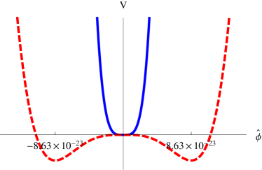
(a)  The potentials at $z=1$

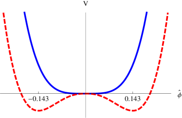
(b)  The potentials at $z=2$

Figure 1: The effective potentials for $z=1$ and $z=2$ are given by Eq. (26) and Eq. (29), respectively. The solid and dashed lines represent the classical($\hbar=0$) and one-loop($\hbar=1$) effective potentials, respectively. The constants have been chosen as $N_{\lambda}=\lambda=\alpha=M_{0}=1$ for simplicity. With these constants, the effective potential has minimal values at $\hat{\phi}=\pm 8.62703\times 10^{-23}$ and $\hat{\phi}=\pm 0.143432$ for $z=1$ and $z=2$, respectively.

II.2 $m^{2}\neq 0$ case

As was done in the previous section, we first obtain the effective potential for the case of $z=1$. Then, the counterterms can be determined in terms of the three dimensional UV cutoff as

$$\delta m_{(1)}^{2} =-\frac{\Lambda^{2}\lambda}{2^{4}\pi^{2}c}-\frac{m^{2}\lambda}{2^{5}\pi^{2}c^{3}}\left(\ln\frac{m^{2}}{4c^{2}\Lambda^{2}}+1\right),$$ (30)

$$\delta\lambda^{(1)} =-\frac{3\lambda^{2}}{2^{5}\pi^{2}c^{3}}\left(\ln\frac{m^{2}}{4c^{2}\Lambda^{2}}+1\right),$$ (31)

where we used $M_{0}=0$ in Eq. (22) since we can avoid the IR divergence with the help of the nonvanishing mass term. Then, the effective potential in the Lorentz invariant scalar field theory is

$$V_{\rm eff}(\hat{\phi})=\frac{1}{2}m^{2}\hat{\phi}^{2}+\frac{\lambda}{4!}\hat{\phi}^{4}+\frac{\hbar}{64\pi^{2}c^{3}}\left[M^{4}\ln\frac{M^{2}}{m^{2}}-\frac{\lambda}{2}\hat{\phi}^{2}\left(m^{2}+\frac{3}{4}\lambda\hat{\phi}^{2}\right)\right],$$ (32)

which agrees with the result for $c=1$ given in Refs. Jackiw:1974cv ; Dolan:1974gu ; Weinberg:1973ua ; Dolan:1973qd ; however, the potential (32) was shifted to satisfy $V_{\text{eff}}(0)=0$.

Next, for a massive Lifshitz scalar field at a fixed point $z=2$, the mass and the coupling constant counterterms from Eqs. (21) and (22) can be determined as

$$\delta m_{(1)}^{2} =-\frac{\Lambda\lambda_{1}}{8\pi^{2}\alpha}+\tilde{m}^{2},$$ (33)

$$\delta\lambda_{n}^{(1)} =-\frac{\Lambda\lambda_{n+1}}{8\pi^{2}\alpha}+\tilde{\lambda}_{n},$$ (34)

where $\tilde{m}^{2}$ and $\tilde{\lambda}_{n}$ are now defined by $\tilde{m}^{2}=[\Gamma(3/4)]^{2}(10\pi^{5/2}\alpha^{3/2})^{-1}(\partial/\partial\hat{\phi})^{2}(M^{2})^{5/4}|_{\hat{\phi}=0}$ and $\tilde{\lambda}_{n}=[\Gamma(3/4)]^{2}(10\pi^{5/2}\alpha^{3/2})^{-1}(\partial/\partial\hat{\phi})^{2n+2}(M^{2})^{5/4}|_{\hat{\phi}=0}$. And then, plugging Eqs. (33) and (34) into Eq. (20), the effective potential can be easily obtained as

$$V_{\rm eff}(\hat{\phi}) =\frac{m^{2}+\hbar\tilde{m}^{2}}{2}\hat{\phi}^{2}+\sum_{n=1}^{4}\frac{(\lambda_{n}+\hbar\tilde{\lambda}_{n})}{(2n+2)!}\hat{\phi}^{2n+2}-\frac{\hbar[\Gamma(3/4)]^{2}}{10\pi^{5/2}\alpha^{3/2}}\left[(M^{2})^{5/4}-(m^{2})^{5/4}\right].$$ (35)

Although the effective potential approximates to the classical potential with renormalized mass and coupling constants for small $\hat{\phi}$, it is hard to say what happens to the effective potential on general ground for $N_{\lambda}>1$. However, simply for $m^{2}>0$ with $N_{\lambda}=1$, there is no symmetry breaking behavior. To see this, we first calculate the slope of Eq. (35) written as

$$\partial V_{\rm eff}(\hat{\phi})/\partial\hat{\phi}=\hat{\phi}f(\hat{\phi}),$$ (36)

where $f(\hat{\phi})=2m^{2}/3+3\lambda\Delta(m^{2})^{1/4}/4+M^{2}/3+\lambda^{2}\Delta(m^{2})^{-3/4}M^{2}/4-\lambda\Delta(M^{2})^{1/4}$ with a positive constant $\Delta\equiv\hbar[\Gamma(3/4)]^{2}/(2^{3}\pi^{5/2}\alpha^{3/2})$. The function $f(\hat{\phi})$ is always positive so that there is no symmetry breaking behavior.

On the other hand, for $m^{2}<0$ corresponding to the case of the classically broken symmetry, the effective potential may be complex depending on the range of field for a given mass so that we have to consider the real part of the effective potential. Then, Eq. (35) can be expressed as

$$V_{\rm eff}(\hat{\phi}) =\frac{m^{2}+\text{Re}(\tilde{m}^{2})}{2^{3/2}}\hat{\phi}^{2}+\sum_{n=1}^{4}\frac{\lambda_{n}+\text{Re}(\tilde{\lambda}_{n})}{(2n+2)!}\hat{\phi}^{2n+2}-\frac{\hbar[\Gamma(3/4)]^{2}}{10\pi^{5/2}\alpha^{3/2}}\left[(M^{2})^{5/4}+\frac{(-m^{2})^{5/4}}{\sqrt{2}}\right],$$ (37)

for $M^{2}>0$, and

$$V_{\rm eff}(\hat{\phi}) =\frac{m^{2}+\text{Re}(\tilde{m}^{2})}{2}\hat{\phi}^{2}+\sum_{n=1}^{4}\frac{\lambda_{n}+\text{Re}(\tilde{\lambda}_{n})}{(2n+2)!}\hat{\phi}^{2n+2}+\frac{\hbar[\Gamma(3/4)]^{2}}{10\sqrt{2}\pi^{5/2}\alpha^{3/2}}\left[(-M^{2})^{5/4}-(-m^{2})^{5/4}\right],$$ (38)

for $M^{2}<0$. As seen from Fig. 2, the vacuum expectation values are quantum mechanically larger than the classical ones, in particular, remarkably for the case of $z=2$.

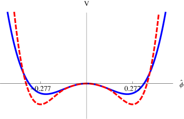
(a)  The potentials at $z=1$

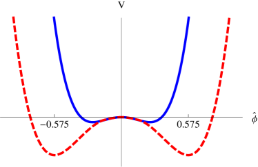
(b)  The potentials at $z=2$

Figure 2: The effective potentials for $z=1$ and $z=2$ are given by Eq. (32) and Eq. (35), respectively. This figure shows the behavior of the effective potential for $m^{2}<0$. The solid and dashed lines represent the classical($\hbar=0$) and one-loop($\hbar=1$) effective potentials, respectively. The constants have been chosen as $m^{2}=-1$, $\lambda=100$ and $N_{\lambda}=\alpha=M_{0}=1$ for simplicity. With these constants, the effective potential has minimal values at $\hat{\phi}=\pm 0.276978$ and $\hat{\phi}=\pm 0.574470$ for $z=1$ and $z=2$, respectively.

III Effective potential at finite temperature

Now, we would like to investigate the critical temperature to give the phase transition from the quantum-mechanically broken vacuum symmetry to the symmetric phase. At a finite temperature $\beta^{-1}$, the time interval is given by $0\leq t\leq-i\beta$. Then, the time component of the four vector $k_{\mu}$ becomes $\omega_{n}=2\pi n/(-i\beta)$, and the effective potential (10) can be written as

$$V_{1}^{\beta}(\hat{\phi^{2}}) =\frac{\hbar}{2\beta}\sum_{n}\int\frac{d^{3}\vec{k}}{(2\pi)^{3}}\ln\left[k_{0}^{2}-\alpha^{2}(\vec{k}^{2})^{2}-\tilde{M}^{2}\right]$$

$$=\frac{\hbar}{2\beta}\sum_{n}\int\frac{d^{3}\vec{k}}{(2\pi)^{3}}\left[-\frac{4\pi^{2}n^{2}}{\beta^{2}}-\tilde{E}_{M}^{2}\right],$$ (39)

where the summation is over $n=0,\pm 1,\pm 2,\cdots$. In order to calculate the summation, we consider

$$v(E)=\sum_{n}\ln\left(\frac{4\pi^{2}n^{2}}{\beta^{2}}+E^{2}\right).$$ (40)

The partial derivative of $v(E)$ with respect to $E$ is given by

$$\frac{\partial v(E)}{\partial E} =\sum_{n}\frac{2E}{4\pi^{2}n^{2}/\beta^{2}+E^{2}}$$

$$=2\beta\left(\frac{1}{2}+\frac{1}{e^{\beta E}-1}\right),$$ (41)

where the second line has been obtained using the equality $\sum_{n=1}^{\infty}\frac{y}{y^{2}+n^{2}}=-\frac{1}{2y}+\frac{\pi}{2}\coth\pi y$. Integrating out Eq. (41) with respect to $E$, we obtain

$$v(E)=2\beta\left[\frac{E}{2}+\frac{1}{\beta}\ln\left(1-e^{-\beta E}\right)\right]+\mathrm{const.}$$ (42)

As a result, the effective potential at the finite temperature in order of $\hbar$,

$$V_{1}^{\beta}(\hat{\phi^{2}}) =\hbar\int\frac{d^{3}\vec{k}}{(2\pi)^{3}}\left[\frac{E_{M}}{2}+\frac{1}{\beta}\ln\left(1-e^{-\beta E_{M}}\right)\right]$$

$$=V_{1}^{0}(\hat{\phi^{2}})+\bar{V}_{1}^{\beta}(\hat{\phi^{2}}),$$ (43)

where the zero-temperature one-loop term $V_{1}^{0}(\hat{\phi^{2}})$ and the temperature-dependent one-loop term $\bar{V}_{1}^{\beta}(\hat{\phi^{2}})$ are

$$V_{1}^{0}(\hat{\phi^{2}}) =\hbar\int\frac{d^{3}\vec{k}}{(2\pi)^{3}}\frac{E_{M}}{2}=\frac{\hbar}{2}\int\frac{d^{3}\vec{k}}{(2\pi)^{3}}\sqrt{\alpha^{2}(\vec{k}^{2})^{2}+M^{2}},$$ (44)

$$\bar{V}_{1}^{\beta}(\hat{\phi^{2}}) =\frac{\hbar}{\beta}\int\frac{d^{3}\vec{k}}{(2\pi)^{3}}\ln\left(1-e^{-\beta E_{M}}\right)$$

$$=\frac{\hbar}{2\pi^{2}\beta}\int_{0}^{\infty}dk\,k^{2}\ln\left(1-e^{-\alpha\beta\sqrt{k^{4}+a^{2}}}\right),$$ (45)

with $a^{2}\equiv M^{2}/\alpha^{2}$. Then, the critical temperature $\beta_{c}$ which recovers the symmetry can be determined by Dolan:1974gu

$$-\frac{m^{2}}{2} =\left.\frac{\partial\bar{V}_{1}^{\beta_{c}}}{\partial\hat{\phi}^{2}}\right|_{\hat{\phi}=0}$$

$$=\frac{\hbar\lambda}{8\pi^{2}\alpha}\int_{0}^{\infty}dk\frac{k^{2}}{\sqrt{k^{4}+m^{2}/\alpha^{2}}\left(e^{\alpha\beta_{c}\sqrt{k^{4}+m^{2}/\alpha^{2}}}-1\right)}.$$ (46)

Note that there is no critical temperature for $m^{2}>0$ since the right hand side in Eq. (46) is always positive due to the positivity of the integrand for the whole range. For $m^{2}=0$, the integrand is divergent. In particular, for $m^{2}<0$, the integral in Eq. (46) would lead to complex values which are unphysical. However, we can avoid the complex values by restricting the range of momentum in Eq. (46) by setting the lower bound as $\epsilon\equiv(-m^{2}/\alpha^{2})^{1/4}$. Unfortunately, the integral is divergent, which means that there is no critical temperature in the one-loop approximation.

IV Discussion

We have studied the four dimensional Lifshitz scalar field theory of the anisotropic scaling of $z=2$, and obtained the renormalized one-loop effective potential. The UV divergence is slightly improved in that the finite counterterm is needed only for the highest order of the coupling constant. For $m^{2}>0$ with $N_{\lambda}=1$, there is no symmetry breaking behavior. For $m^{2}<0$ , the overall behavior of the effective potential of $z=2$ is analogous to that of $z=1$; however, the vacuum expectation value is significantly larger than the classical vacuum expectation value. Unfortunately, the critical temperatures can not be obtained in this one-loop approximation.

On the other hand, if one considers the most general action of Eq. (2) with the counterterms given by $\mathcal{L}_{ct}=-\delta m^{2}\phi^{2}/2-\sum_{n=1}^{N_{\lambda}}\delta\lambda_{n}\phi^{2n+2}/(2n+2)!$, the mass and the coupling constant counterterms are calculated as $\delta m_{(1)}^{2}=-\Lambda^{3}\eta_{1}/(24\pi^{2}\alpha)-\Lambda(4\alpha^{2}\lambda_{1}-c^{2}\eta_{1})/(32\pi^{2}\alpha^{3})+\tilde{m}^{2}$, $\delta\lambda_{1}^{(1)}=-\Lambda^{3}\eta_{2}/(24\pi^{2}\alpha)-\Lambda(48\alpha^{2}\lambda_{2}-3\eta_{1}^{2}-c^{2}\eta_{2})/(3\cdot 2^{7}\pi^{2}\alpha^{3})+\tilde{\lambda}_{1}$, $\delta\lambda_{2}^{(1)}=-\Lambda(2\alpha^{2}\lambda_{2}-15\eta_{1}\eta_{2})/(16\pi^{2}\alpha^{3})+\tilde{\lambda}_{2}$, $\delta\lambda_{3}^{(1)}=-\Lambda(2\alpha^{2}\lambda_{2}-35\eta_{2}^{2})/(16\pi^{2}\alpha^{3})+\tilde{\lambda}_{3}$, and $\delta\lambda_{4}^{(1)}=\tilde{\lambda}_{4}$, where $\tilde{m}^{2}$ and $\tilde{\lambda}_{n}$’s are just finite constants. Unfortunately, we can not exhibit the effective potential, $\tilde{m}^{2}$ and $\tilde{\lambda}_{n}$ explicitly because they are so lengthy. However, it is interesting to note that the highest order of coupling constant counterterm $\delta\lambda_{4}^{(1)}$ is still independent of the UV cutoff. Furthermore, taking the limit of $c\to 0$ and $\eta_{n}\to 0$, the above counterterms become exactly the same as Eqs. (27) and (28), while they are not compatible with those of the $z=1$ case because the limit of $\alpha\to 0$ is ill-defined.

- (1) P. Hořava, JHEP 0903 (2009) 020 [arXiv:0812.4287 [hep-th]].
- (2) P. Hořava, Phys. Rev. D 79 (2009) 084008 [arXiv:0901.3775 [hep-th]].
- (3) H. Lu, J. Mei and C. N. Pope, Phys. Rev. Lett. 103 (2009) 091301 [arXiv:0904.1595 [hep-th]].
- (4) R. G. Cai, L. M. Cao and N. Ohta, Phys. Lett. B 679 (2009) 504 [arXiv:0905.0751 [hep-th]].
- (5) A. Ghodsi, E. Hatefi, Phys. Rev. D81 (2010) 044016. [arXiv:0906.1237 [hep-th]].
- (6) G. Koutsoumbas, E. Papantonopoulos, P. Pasipoularides and M. Tsoukalas, Phys. Rev. D 81 (2010) 124014 [arXiv:1004.2289 [hep-th]].
- (7) G. Koutsoumbas and P. Pasipoularides, Phys. Rev. D 82 (2010) 044046 [arXiv:1006.3199 [hep-th]].
- (8) M. Eune and W. Kim, Phys. Rev. D 82 (2010) 124048 [arXiv:1007.1824 [hep-th]].
- (9) I. Radinschi, F. Rahaman and A. Banerjee, arXiv:1012.0986 [gr-qc].
- (10) E. Kiritsis and G. Kofinas, Nucl. Phys. B 821 (2009) 467 [arXiv:0904.1334 [hep-th]].
- (11) S. Mukohyama, JCAP 0906 (2009) 001 [arXiv:0904.2190 [hep-th]].
- (12) S. Mukohyama, K. Nakayama, F. Takahashi and S. Yokoyama, Phys. Lett. B 679 (2009) 6 [arXiv:0905.0055 [hep-th]].
- (13) R. Brandenberger, Phys. Rev. D 80 (2009) 043516 [arXiv:0904.2835 [hep-th]].
- (14) M. R. Setare and M. Jamil, JCAP 1002 (2010) 010 [Erratum-ibid. 1008 (2010) E01] [arXiv:1001.1251 [hep-th]].
- (15) M. Jamil, E. N. Saridakis and M. R. Setare, JCAP 1011 (2010) 032 [arXiv:1003.0876 [hep-th]].
- (16) E. J. Son and W. Kim, JCAP 1006 (2010) 025 [arXiv:1003.3055 [hep-th]].
- (17) K. Balasubramanian and K. Narayan, JHEP 1008 (2010) 014 [arXiv:1005.3291 [hep-th]].
- (18) K. Saaidi and A. Aghamohammadi, Astrophys. Space Sci. 332 (2011) 503 [arXiv:1006.1834 [gr-qc]].
- (19) K. Maeda, Y. Misonoh and T. Kobayashi, Phys. Rev. D 82 (2010) 064024 [arXiv:1006.2739 [hep-th]].
- (20) E. N. Saridakis, arXiv:1101.0300 [astro-ph.CO].
- (21) E. M. Lifshitz, Zh. Eksp. Teor. Fiz. 11 (1941) 255; Zh. Eksp. Teor. Fiz. 11 (1941) 269.
- (22) R. M. Hornreich, M. Luban and S. Shtrikman, Phys. Rev. Lett. 35 (1975) 1678.
- (23) P. Hořava, Phys. Lett. B 694 (2010) 172 [arXiv:0811.2217 [hep-th]].
- (24) R. Iengo, J. G. Russo, M. Serone, JHEP 0911 (2009) 020. [arXiv:0906.3477 [hep-th]].
- (25) S. R. Coleman, E. J. Weinberg, Phys. Rev. D7 (1973) 1888-1910.
- (26) S. Weinberg, Phys. Rev. D7 (1973) 2887-2910.
- (27) L. A. Dolan, R. Jackiw, Phys. Rev. D9 (1974) 2904.
- (28) R. Jackiw, Phys. Rev. D9 (1974) 1686.
- (29) L. A. Dolan, R. Jackiw, Phys. Rev. D9, 3320-3341 (1974).
- (30) R. H. Brandenberger, Rev. Mod. Phys. 57 (1985) 1.