Misleading Stars: What Cannot Be Measured in the Internet?

Abstract

Traceroute measurements are one of our main instruments to shed light onto the structure and properties of today’s complex networks such as the Internet. This paper studies the feasibility and infeasibility of inferring the network topology given traceroute data from a worst-case perspective, i.e., without any probabilistic assumptions on, e.g., the nodes’ degree distribution. We attend to a scenario where some of the routers are anonymous, and propose two fundamental axioms that model two basic assumptions on the traceroute data: (1) each trace corresponds to a real path in the network, and (2) the routing paths are at most a factor $1/\alpha$ off the shortest paths, for some parameter $\alpha\in(0,1]$. In contrast to existing literature that focuses on the cardinality of the set of (often only minimal) inferrable topologies, we argue that a large number of possible topologies alone is often unproblematic, as long as the networks have a similar structure. We hence seek to characterize the set of topologies inferred with our axioms. We introduce the notion of star graphs whose colorings capture the differences among inferred topologies; it also allows us to construct inferred topologies explicitly. We find that in general, inferrable topologies can differ significantly in many important aspects, such as the nodes’ distances or the number of triangles. These negative results are complemented by a discussion of a scenario where the trace set is best possible, i.e., “complete”. It turns out that while some properties such as the node degrees are still hard to measure, a complete trace set can help to determine global properties such as the connectivity.

1 Introduction

Surprisingly little is known about the structure of many important complex networks such as the Internet. One reason is the inherent difficulty of performing accurate, large-scale and preferably synchronous measurements from a large number of different vantage points. Another reason are privacy and information hiding issues: for example, network providers may seek to hide the details of their infrastructure to avoid tailored attacks.

Since knowledge of the network characteristics is crucial for many applications (e.g., RMTP [12], or PaDIS [13]), the research community implements measurement tools to analyze at least the main properties of the network. The results can then, e.g., be used to design more efficient network protocols in the future.

This paper focuses on the most basic characteristic of the network: its topology. The classic tool to study topological properties is traceroute. Traceroute allows us to collect traces from a given source node to a set of specified destination nodes. A trace between two nodes contains a sequence of identifiers describing the route traveled by the packet. However, not every node along such a path is configured to answer with its identifier. Rather, some nodes may be anonymous in the sense that they appear as stars (‘$*$’) in a trace. Anonymous nodes exacerbate the exploration of a topology because already a small number of anonymous nodes may increase the spectrum of inferrable topologies that correspond to a trace set $\mathcal{T}$.

This paper is motivated by the observation that the mere number of inferrable topologies alone does not contradict the usefulness or feasibility of topology inference; if the set of inferrable topologies is homogeneous in the sense that that the different topologies share many important properties, the generation of all possible graphs can be avoided: an arbitrary representative may characterize the underlying network accurately. Therefore, we identify important topological metrics such as diameter or maximal node degree and examine how “close” the possible inferred topologies are with respect to these metrics.

1.1 Related Work

Arguably one of the most influential measurement studies on the Internet topology was conducted by the Faloutsos brothers [8] who show that the Internet exhibits a skewed structure: the nodes’ out-degree follows a power-law distribution. Moreover, this property seems to be invariant over time. These results complement discoveries of similar distributions of communication traffic which is often self-similar, and of the topologies of natural networks such as human respiratory systems. This property allows us to give good predictions not only on node degree distributions but also, e.g., on the expected number of nodes at a given hop-distance. Since [8] was published, many additional results have been obtained, e.g., by conducting a distributed computing approach to increase the number of measurement points [6]. However, our understanding remains preliminary, and the topic continues to attract much attention from the scientific communities. In contrast to these measurement studies, we pursue a more formal approach, and a complete review of the empirical results obtained over the last years is beyond the scope of this paper.

In the field of network tomography, topologies are explored using pairwise end-to-end measurements, without the cooperation of nodes along these paths. This approach is quite flexible and applicable in various contexts, e.g., in social networks [4]. For a good discussion of this approach as well as results for a routing model along shortest and second shortest paths see [4]. For example, [4] shows that for sparse random graphs, a relatively small number of cooperating participants is sufficient to discover a network fairly well.

The classic tool to discover Internet topologies is traceroute [7]. Unfortunately, there are several problems with this approach that render topology inference difficult, such as aliasing or load-balancing, which has motivated researchers to develop new tools such as Paris Traceroute [5, 10]. Another complication stems from the fact that routers may appear as stars in the trace since they are overloaded or since they are configured not to send out any ICMP responses. The lack of complete information in the trace set renders the accurate characterization of Internet topologies difficult.

This paper attends to the problem of anonymous nodes and assumes a conservative, “worst-case” perspective that does not rely on any assumptions on the underlying network. There are already several works on the subject. Yao et al. [15] initiated the study of possible candidate topologies for a given trace set and suggested computing the minimal topology, that is, the topology with the minimal number of anonymous nodes, which turns out to be NP-hard. Consequently, different heuristics have been proposed [9, 10].

Our work is motivated by a series of papers by Acharya and Gouda. In [3], a network tracing theory model is introduced where nodes are “irregular” in the sense that each node appears in at least one trace with its real identifier. In [1], hardness results are derived for this model. However, as pointed out by the authors themselves, the irregular node model—where nodes are anonymous due to high loads—is less relevant in practice and hence they consider strictly anonymous nodes in their follow-up studies [2]. As proved in [2], the problem is still hard (in the sense that there are many minimal networks corresponding to a trace set), even with only two anonymous nodes, symmetric routing and without aliasing.

In contrast to this line of research on cardinalities, we are interested in the network properties. If the inferred topologies share the most important characteristics, the negative results in [1, 2] may be of little concern. Moreover, we believe that a study limited to minimal topologies only may miss important redundancy aspects of the Internet. Unlike [1, 2], our work is constructive in the sense that algorithms can be derived to compute inferred topologies.

1.2 Our Contribution

This paper initiates the study and characterization of topologies that can be inferred from a given trace set computed with the traceroute tool. While existing literature assuming a worst-case perspective has mainly focused on the cardinality of minimal topologies, we go one step further and examine specific topological graph properties.

We introduce a formal theory of topology inference by proposing basic axioms (i.e., assumptions on the trace set) that are used to guide the inference process. We present a novel and we believe appealing definition for the isomorphism of inferred topologies which is aware of traffic paths; it is motivated by the observation that although two topologies look equivalent up to a renaming of anonymous nodes, the same trace set may result in different paths. Moreover, we initiate the study of two extremes: in the first scenario, we only require that each link appears at least once in the trace set; interestingly, however, it turns out that this is often not sufficient, and we propose a “best case” scenario where the trace set is, in some sense, complete: it contains paths between all pairs of nodes.

The main result of the paper is a negative one. It is shown that already a small number of anonymous nodes in the network renders topology inference difficult. In particular, we prove that in general, the possible inferrable topologies differ in many crucial aspects.

We introduce the concept of the star graph of a trace set that is useful for the characterization of inferred topologies. In particular, colorings of the star graphs allow us to constructively derive inferred topologies. (Although the general problem of computing the set of inferrable topologies is related to NP-hard problems such as minimal graph coloring and graph isomorphism, some important instances of inferrable topologies can be computed efficiently.) The minimal coloring (i.e., the chromatic number) of the star graph defines a lower bound on the number of anonymous nodes from which the stars in the traces could originate from. And the number of possible colorings of the star graph—a function of the chromatic polynomial of the star graph—gives an upper bound on the number of inferrable topologies. We show that this bound is tight in the sense that there are situation where there indeed exist so many inferrable topologies. Especially, there are problem instances where the cardinality of the set of inferrable topologies equals the Bell number. This insight complements (and generalizes to arbitrary, not only minimal, inferrable topologies) existing cardinality results.

Finally, we examine the scenario of fully explored networks for which “complete” trace sets are available. As expected, inferrable topologies are more homogenous and can be characterized well with respect to many properties such as node distances. However, we also find that other properties are inherently difficult to estimate. Interestingly, our results indicate that full exploration is often useful for global properties (such as connectivity) while it does not help much for more local properties (such as node degree).

1.3 Organization

The remainder of this paper is organized as follows. Our theory of topology inference is introduced in Section 2. The main contribution is presented in Sections 3 and 4 where we derive bounds for general trace sets and fully explored networks, respectively. In Section 5, the paper concludes with a discussion of our results and directions for future research. Due to space constraints, some proofs are moved to the appendix.

2 Model

Let $\mathcal{T}$ denote the set of traces obtained from probing (e.g., by traceroute) a (not necessarily connected and undirected) network $G_{0}=(V_{0},E_{0})$ with nodes or vertices $V_{0}$ (the set of routers) and links or edges $E_{0}$. We assume that $G_{0}$ is static during the probing time (or that probing is instantaneous). Each trace $T(u,v)\in\mathcal{T}$ describes a path connecting two nodes $u,v\in V_{0}$; when $u$ and $v$ do not matter or are clear from the context, we simply write $T$. Moreover, let $d_{T}(u,v)$ denote the distance (number of hops) between two nodes $u$ and $v$ in trace $T$. We define $d_{G_{0}}(u,v)$ to be the corresponding shortest path distance in $G_{0}$. Note that a trace between two nodes $u$ and $v$ may not describe the shortest path between $u$ and $v$ in $G_{0}$.

The nodes in $V_{0}$ fall into two categories: anonymous nodes and non-anonymous (or shorter: named) nodes. Therefore, each trace $T\in\mathcal{T}$ describes a sequence of symbols representing anonymous and non-anonymous nodes. We make the natural assumption that the first and the last node in each trace $T$ is non-anonymous. Moreover, we assume that traces are given in a form where non-anonymous nodes appear with a unique, anti-aliased identifier (i.e., the multiple IP addresses corresponding to different interfaces of a node are resolved to one identifier); an anonymous node is represented as $*$ (“star”) in the traces. For our formal analysis, we assign to each star in a trace set $\mathcal{T}$ a unique identifier $i$: $*_{i}$. (Note that except for the numbering of the stars, we allow identical copies of $T$ in $\mathcal{T}$, and we do not make any assumptions on the implications of identical traces: they may or may not describe the same paths.) Thus, a trace $T\in\mathcal{T}$ is a sequence of symbols taken from an alphabet $\Sigma=\mathcal{ID}\cup\left(\bigcup_{i}*_{i}\right)$, where $\mathcal{ID}$ is the set of non-anonymous node identifiers (IDs): $\Sigma$ is the union of the (anti-aliased) non-anonymous nodes and the set of all stars (with their unique identifiers) appearing in a trace set. The main challenge in topology inference is to determine which stars in the traces may originate from which anonymous nodes.

Henceforth, let $n=|\mathcal{ID}|$ denote the number of non-anonymous nodes and let $s=\left|\bigcup_{i}*_{i}\right|$ be the number of stars in $\mathcal{T}$; similarly, let $a$ denote the number of anonymous nodes in a topology. Let $N=n+s=|\Sigma|$ be the total number of symbols occurring in $\mathcal{T}$.

Clearly, the process of topology inference depends on the assumptions on the measurements. In the following, we postulate the fundamental axioms that guide the reconstruction. First, we make the assumption that each link of $G_{0}$ is visited by the measurement process, i.e., it appears as a transition in the trace set $\mathcal{T}$. In other words, we are only interested in inferring the (sub-)graph for which measurement data is available.

Axiom 0 (Complete Cover): Each edge of $G_{0}$ appears at least once in some trace in $\mathcal{T}$.

The next fundamental axiom assumes that traces always represent paths on $G_{0}$.

Axiom 1 (Reality Sampling): For every trace $T\in\mathcal{T}$, if the distance between two symbols $\sigma_{1},\sigma_{2}\in T$ is $d_{T}(\sigma_{1},\sigma_{2})=k$, then there exists a path (i.e., a walk without cycles) of length $k$ connecting two (named or anonymous) nodes $\sigma_{1}$ and $\sigma_{2}$ in $G_{0}$.

The following axiom captures the consistency of the routing protocol on which the traceroute probing relies. In the current Internet, policy routing is known to have in impact both on the route length [14] and on the convergence time [11].

Axiom 2 ($\alpha$-(Routing) Consistency): There exists an $\alpha\in(0,1]$ such that, for every trace $T\in\mathcal{T}$, if $d_{T}(\sigma_{1},\sigma_{2})=k$ for two entries $\sigma_{1},\sigma_{2}$ in trace $T$, then the shortest path connecting the two (named or anonymous) nodes corresponding to $\sigma_{1}$ and $\sigma_{2}$ in $G_{0}$ has distance at least $\lceil\alpha k\rceil$.

Note that if $\alpha=1$, the routing is a shortest path routing. Moreover, note that if $\alpha=0$, there can be loops in the paths, and there are hardly any topological constraints, rendering almost any topology inferrable. (For example, the complete graph with one anonymous router is always a solution.)

A natural axiom to merge traces is the following.

Axiom 3 (Trace Merging): For two traces $T_{1},T_{2}\in\mathcal{T}$ for which $\exists\sigma_{1},\sigma_{2},\sigma_{3}$, where $\sigma_{2}$ refers to a named node, such that $d_{T_{1}}(\sigma_{1},\sigma_{2})=i$ and $d_{T_{2}}(\sigma_{2},\sigma_{3})=j$, it holds that the distance between two nodes $u$ and $v$ corresponding to $\sigma_{1}$ and $\sigma_{2}$, respectively, in $G_{0}$, is at most $d_{G_{0}}(\sigma_{1},\sigma_{3})\leq i+j$.

Any topology $G$ which is consistent with these axioms (when applied to $\mathcal{T}$) is called inferrable from $\mathcal{T}$.

Definition 2.1 (Inferrable Topologies).

A topology $G$ is ($\alpha$-consistently) inferrable from a trace set $\mathcal{T}$ if axioms Axiom 0, Axiom 1, Axiom 2 (with parameter $\alpha$), and Axiom 3 are fulfilled.

We will refer by $\mathcal{G}_{\mathcal{T}}$ to the set of topologies inferrable from $\mathcal{T}$. Please note the following important observation.

Remark 2.2.

While we generally have that $G_{0}\in\mathcal{G}_{\mathcal{T}}$, since $\mathcal{T}$ was generated from $G_{0}$ and Axiom 0, Axiom 1, Axiom 2  and Axiom 3 are fulfilled by definition, there can be situations where an $\alpha$-consistent trace set for $G_{0}$ contradicts Axiom 0: some edges may not appear in $\mathcal{T}$. If this is the case, we will focus on the inferrable topologies containing the links we know, even if $G_{0}$ may have additional, hidden links that cannot be explored due to the high $\alpha$ value.

The main objective of a topology inference algorithm Alg is to compute topologies which are consistent with these axioms. Concretely, Alg’s input is the trace set $\mathcal{T}$ together with the parameter $\alpha$ specifying the assumed routing consistency. Essentially, the goal of any topology inference algorithm Alg is to compute a mapping of the symbols $\Sigma$ (appearing in $\mathcal{T}$) to nodes in an inferred topology $G$; or, in case the input parameters $\alpha$ and $\mathcal{T}$ are contradictory, reject the input. This mapping of symbols to nodes implicitly describes the edge set of $G$ as well: the edge set is unique as all the transitions of the traces in $\mathcal{T}$ are now unambiguously tied to two nodes.

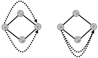
Figure 1: Two non-isomorphic inferred topologies, i.e., different mapping functions lead to these topologies.

So far, we have ignored an important and non-trivial question: When are two topologies $G_{1},G_{2}\in\mathcal{G}_{\mathcal{T}}$ different (and hence appear as two independent topologies in $\mathcal{G}_{\mathcal{T}}$)? In this paper, we pursue the following approach: We are not interested in purely topological isomorphisms, but we care about the identifiers of the non-anonymous nodes, i.e., we are interested in the locations of the non-anonymous nodes and their distance to other nodes. For anonymous nodes, the situation is slightly more complicated: one might think that as the nodes are anonymous, their “names” do not matter. Consider however the example in Figure 1: the two inferrable topologies have two anonymous nodes, once where $\{*_{1},*_{2}\}$ plus $\{*_{3},*_{4}\}$ are merged into one node each in the inferrable topology and once where $\{*_{1},*_{4}\}$ plus $\{*_{2},*_{3}\}$ are merged into one node each in the inferrable topology. In this paper, we regard the two topologies as different, for the following reason: Assume that there are two paths in the network, one $u\rightsquigarrow*_{2}\rightsquigarrow v$ (e.g., during day time) and one $u\rightsquigarrow*_{3}\rightsquigarrow v$ (e.g., at night); clearly, this traffic has different consequences and hence we want to be able to distinguish between the two topologies described above. In other words, our notion of isomorphism of inferred topologies is path-aware.

It is convenient to introduce the following Map function. Essentially, an inference algorithm computes such a mapping.

Definition 2.3 (Mapping Function Map).

Let $G=(V,E)\in\mathcal{G}_{\mathcal{T}}$ be a topology inferrable from $\mathcal{T}$. A topology inference algorithm describes a surjective mapping function $\textsc{Map}:\Sigma\to V$. For the set of non-anonymous nodes in $\Sigma$, the mapping function is bijective; and each star is mapped to exactly one node in $V$, but multiple stars may be assigned to the same node. Note that for any $\sigma\in\Sigma$, $\textsc{Map}(\sigma)$ uniquely identifies a node $v\in V$. More specifically, we assume that Map assigns labels to the nodes in $V$: in case of a named node, the label is simply the node’s identifier; in case of anonymous nodes, the label is $*_{\beta}$, where $\beta$ is the concatenation of the sorted indices of the stars which are merged into node $*_{\beta}$.

With this definition, two topologies $G_{1},G_{2}\in\mathcal{G}_{\mathcal{T}}$ differ if and only if they do not describe the identical (Map-) labeled topology. We will use this Map function also for $G_{0}$, i.e., we will write $\textsc{Map}(\sigma)$ to refer to a symbol $\sigma$’s corresponding node in $G_{0}$.

In the remainder of this paper, we will often assume that Axiom 0 is given. Moreover, note that Axiom 3 is redundant. Therefore, in our proofs, we will not explicitly cover Axiom 0, and it is sufficient to show that Axiom 1 holds to prove that Axiom 3 is satisfied.

Lemma 2.4.

Axiom 1 implies Axiom 3.

Proof.

Let $\mathcal{T}$ be a trace set, and $G\in\mathcal{G}_{\mathcal{T}}$. Let $\sigma_{1},\sigma_{2},\sigma_{3}$ s.t. $\exists T_{1},T_{2}\in\mathcal{T}$ with $\sigma_{1}\in T_{1},\sigma_{3}\in T_{2}$ and $\sigma_{2}\in T_{1}\cap T_{2}$. Let $i=d_{T_{1}}(\sigma_{1},\sigma_{2})$ and $j=d_{T_{2}}(\sigma_{1},\sigma_{3})$. Since any inferrable topology $G$ fulfills Axiom 1, there is a path $\pi_{1}$ of length at most $i$ between the nodes corresponding to $\sigma_{1}$ and $\sigma_{2}$ in $G$ and a path $\pi_{2}$ of length at most $j$ between the nodes corresponding to $\sigma_{2}$ and $\sigma_{3}$ in $G$. The combined path can only be shorter, and hence the claim follows. ∎

3 Inferrable Topologies

What insights can be obtained from topology inference with minimal assumptions, i.e., with our axioms? Or what is the structure of the inferrable topology set $\mathcal{G}_{\mathcal{T}}$? We first make some general observations and then examine different graph metrics in more detail.

3.1 Basic Observations

Although the generation of the entire topology set $\mathcal{G}_{\mathcal{T}}$ may be computationally hard, some instances of $\mathcal{G}_{\mathcal{T}}$ can be computed efficiently. The simplest possible inferrable topology is the so-called canonic graph $G_{C}$: the topology which assumes that all stars in the traces refer to different anonymous nodes. In other words, if a trace set $\mathcal{T}$ contains $n=|\mathcal{ID}|$ named nodes and $s$ stars, $G_{C}$ will contain $|V(G_{C})|=N=n+s$ nodes.

Definition 3.1 (Canonic Graph $G_{C}$).

The canonic graph is defined by $G_{C}(V_{C},E_{C})$ where $V_{C}=\Sigma$ is the set of (anti-aliased) nodes appearing in $\mathcal{T}$ (where each star is considered a unique anonymous node) and where $\{\sigma_{1},\sigma_{2}\}\in E_{C}\Leftrightarrow\exists T\in\mathcal{T},T=(\ldots,\sigma_{1},\sigma_{2},\ldots)$, i.e., $\sigma_{1}$ follows after $\sigma_{2}$ in some trace $T$ ($\sigma_{1},\sigma_{2}\in T$ can be either non-anonymous nodes or stars). Let $d_{C}(\sigma_{1},\sigma_{2})$ denote the canonic distance between two nodes, i.e., the length of a shortest path in $G_{C}$ between the nodes $\sigma_{1}$ and $\sigma_{2}$.

Note that $G_{C}$ is indeed an inferrable topology. In this case, $\textsc{Map}:\Sigma\rightarrow\Sigma$ is the identity function. The proof appears in the appendix.

Theorem 3.2.

$G_{C}$ is inferrable from $\mathcal{T}$.

$G_{C}$ can be computed efficiently from $\mathcal{T}$: represent each non-anonymous node and star as a separate node, and for any pair of consecutive entries (i.e., nodes) in a trace, add the corresponding link. The time complexity of this construction is linear in the size of $\mathcal{T}$.

With the definition of the canonic graph, we can derive the following lemma which establishes a necessary condition when two stars cannot represent the same node in $G_{0}$ from constraints on the routing paths. This is useful for the characterization of inferred topologies.

Lemma 3.3.

Let $*_{1},*_{2}$ be two stars occurring in some traces in $\mathcal{T}$. $*_{1},*_{2}$ cannot be mapped to the same node, i.e., $\textsc{Map}(*_{1})\neq\textsc{Map}(*_{2})$, without violating the axioms in the following conflict situations:

• if $*_{1}\in T_{1}$ and $*_{2}\in T_{2}$, and $T_{1}$ describes a too long path between anonymous node $\textsc{Map}(*_{1})$ and non-anonymous node $u$, i.e., $\lceil\alpha\cdot d_{T_{1}}(*_{1},u)\rceil>d_{C}(u,*_{2})$.

• if $*_{1}\in T_{1}$ and $*_{2}\in T_{2}$, and there exists a trace $T$ that contains a path between two non-anonymous nodes $u$ and $v$ and $\lceil\alpha\cdot d_{T}(u,v)\rceil>d_{C}(u,*_{1})+d_{C}(v,*_{2}).$

Proof.

The first proof is by contradiction. Assume $\textsc{Map}(*_{1})=\textsc{Map}(*_{2})$ represents the same node $v$ of $G_{0}$, and that $\lceil\alpha\cdot d_{T_{1}}(v,u)\rceil>d_{C}(u,v)$. Then we know from Axiom 2 that $d_{C}(v,u)\geq d_{G_{0}}(v,u)\geq\lceil\alpha\cdot d_{T_{1}}(u,v)\rceil>d_{C}(v,u)$, which yields the desired contradiction.

Similarly for the second proof. Assume for the sake of contradiction that $\textsc{Map}(*_{1})=\textsc{Map}(*_{2})$ represents the same node $w$ of $G_{0}$, and that $\lceil\alpha\cdot d_{T}(u,v)\rceil>d_{C}(u,w)+d_{C}(v,w)$. Due to the triangle inequality, we have that $d_{C}(u,w)+d_{C}(v,w)\geq d_{C}(u,v)$ and hence, $\lceil\alpha\cdot d_{T}(u,v)\rceil>d_{C}(u,v)$, which contradicts the fact that $G_{C}$ is inferrable (Theorem 3.2). ∎

Lemma 3.3 can be applied to show that a topology is not inferrable from a given trace set because it merges (i.e., maps to the same node) two stars in a manner that violates the axioms. Let us introduce a useful concept for our analysis: the star graph that describes the conflicts between stars.

Definition 3.4 (Star Graph $G_{*}$).

The star graph $G_{*}(V_{*},E_{*})$ consists of vertices $V_{*}$ representing stars in traces, i.e., $V_{*}=\bigcup_{i}*_{i}$. Two vertices are connected if and only if they must differ according to Lemma 3.3, i.e., $\{*_{1},*_{2}\}\in E_{*}$ if and only if at least one of the conditions of Lemma 3.3 hold for $*_{1},*_{2}$.

Note that the star graph $G_{*}$ is unique and can be computed efficiently for a given trace set $\mathcal{T}$: Conditions (i) and (ii) can be checked by computing $G_{C}$. However, note that while $G_{*}$ specifies some stars which cannot be merged, the construction is not sufficient: as Lemma 3.3 is based on $G_{C}$, additional links might be needed to characterize the set of inferrable and $\alpha$-consistent topologies $\mathcal{G}_{\mathcal{T}}$ exactly. In other words, a topology $G$ obtained by merging stars that are adjacent in $G_{*}$ is never inferrable ($G\not\in\mathcal{G}_{\mathcal{T}}$); however, merging non-adjacent stars does not guarantee that the resulting topology is inferrable.

What do star graphs look like? The answer is arbitrarily: the following lemma states that the set of possible star graphs is equivalent to the class of general graphs. This claim holds for any $\alpha$. The proof appears in the appendix.

Lemma 3.5.

For any graph $G=(V,E)$, there exists a trace set $\mathcal{T}$ such that $G$ is the star graph for $\mathcal{T}$.

The problem of computing inferrable topologies is related to the vertex colorings of the star graphs. We will use the following definition which relates a vertex coloring of $G_{*}$ to an inferrable topology $G$ by contracting independent stars in $G_{*}$ to become one anonymous node in $G$. For example, observe that a maximum coloring treating every star in the trace as a separate anonymous node describes the inferrable topology $G_{C}$.

Definition 3.6 (Coloring-Induced Graph).

Let $\gamma$ denote a coloring of $G_{*}$ which assigns colors $1,\ldots,k$ to the vertices of $G_{*}$: $\gamma:V_{*}\rightarrow\{1,\ldots,k\}$. We require that $\gamma$ is a proper coloring of $G_{*}$, i.e., that different anonymous nodes are assigned different colors: $\{u,v\}\in E_{*}\Rightarrow\gamma(u)\neq\gamma(v)$. $G_{\gamma}$ is defined as the topology induced by $\gamma$. $G_{\gamma}$ describes the graph $G_{C}$ where nodes of the same color are contracted: two vertices $u$ and $v$ represent the same node in $G_{\gamma}$, i.e., $\textsc{Map}(*_{i})=\textsc{Map}(*_{j})$, if and only if $\gamma(*_{i})=\gamma(*_{j})$.

The following two lemmas establish an intriguing relationship between colorings of $G_{*}$ and inferrable topologies. Also note that Definition 3.6 implies that two different colorings of $G_{*}$ define two non-isomorphic inferrable topologies.

We first show that while a coloring-induced topology always fulfills Axiom 1, the routing consistency is sacrificed. The proof appears in the appendix.

Lemma 3.7.

Let $\gamma$ be a proper coloring of $G_{*}$. The coloring induced topology $G_{\gamma}$ is a topology fulfilling Axiom 2 with a routing consistency of $\alpha^{\prime}$, for some positive $\alpha^{\prime}$.

An inferrable topology always defines a proper coloring on $G_{*}$.

Lemma 3.8.

Let $\mathcal{T}$ be a trace set and $G_{*}$ its corresponding star graph. If a topology $G$ is inferrable from $\mathcal{T}$, then $G$ induces a proper coloring on $G_{*}$.

Proof.

For any $\alpha$-consistent inferrable topology $G$ there exists some mapping function Map that assigns each symbol of $\mathcal{T}$ to a corresponding node in $G$ (cf Definition 2.3), and this mapping function gives a coloring on $G_{*}$ (i.e., merged stars appear as nodes of the same color in $G_{*}$). The coloring must be proper: due to Lemma 3.3, an inferrable topology can never merge adjacent nodes of $G_{*}$. ∎

The colorings of $G_{*}$ allow us to derive an upper bound on the cardinality of $\mathcal{G}_{\mathcal{T}}$.

Theorem 3.9.

Given a trace set $\mathcal{T}$ sampled from a network $G_{0}$ and $\mathcal{G}_{\mathcal{T}}$, the set of topologies inferrable from $\mathcal{T}$, it holds that:

$$\sum_{k=\gamma(G_{*})}^{|V_{*}|}P(G_{*},k)/k!\geq|\mathcal{G}_{\mathcal{T}}|,$$

where $\gamma(G_{*})$ is the chromatic number of $G_{*}$ and $P(G_{*},k)$ is the number of colorings of $G_{*}$ with $k$ colors (known as the chromatic polynomial of $G_{*}$).

Proof.

The proof follows directly from Lemma 3.8 which shows that each inferred topology has proper colorings, and the fact that a coloring of $G_{*}$ cannot result in two different inferred topologies, as the coloring uniquely describes which stars to merge (Lemma 3.7). In order to account for isomorphic colorings, we need to divide by the number of color permutations. ∎

Note that the fact that $G_{*}$ can be an arbitrary graph (Lemma 3.5) implies that we cannot exploit some special properties of $G_{*}$ to compute colorings of $G_{*}$ and $\gamma(G_{*})$. Also note that the exact computation of the upper bound is hard, since the minimal coloring as well as the chromatic polynomial of $G_{*}$ (in P$\sharp$) is needed. To complement the upper bound, we note that star graphs with a small number of conflict edges can indeed result in a large number of inferred topologies.

Theorem 3.10.

For any $\alpha>0$, there is a trace set for which the number of non-isomorphic colorings of $G_{*}$ equals $|\mathcal{G}_{\mathcal{T}}|$, in particular $|\mathcal{G}_{\mathcal{T}}|=B_{s}$, where $\mathcal{G}_{\mathcal{T}}$ is the set of inferrable and $\alpha$-consistent topologies, $s$ is the number of stars in $\mathcal{T}$, and $B_{s}$ is the Bell number of $s$. Such a trace set can originate from a $G_{0}$ network with one anonymous node only.

Proof.

Consider a trace set $\mathcal{T}=\{(\sigma_{i},*_{i},\sigma^{\prime}_{i})_{i=1,\ldots,s}\}$ (e.g., obtained from exploring a topology $G_{0}$ where one anonymous center node is connected to $2s$ named nodes). The trace set does not impose any constraints on how the stars relate to each other, and hence, $G_{*}$ does not contain any edges at all; even when stars are merged, there are no constraints on how the stars relate to each other. Therefore, the star graph for $\mathcal{T}$ has $B_{s}=\sum_{j=0}^{s}S_{(s,j)}$ colorings, where $S_{(s,j)}=1/j!\cdot\sum_{\ell=0}^{j}(-1)^{\ell}\binom{j}{\ell}(j-\ell)^{s}$ is the number of ways to group $s$ nodes into $j$ different, disjoint non-empty subsets (known as the Stirling number of the second kind). Each of these colorings also describes a distinct inferrable topology as Map assigns unique labels to anonymous nodes stemming from merging a group of stars (cf Definition 2.3). ∎

3.2 Properties

Even if the number of inferrable topologies is large, topology inference can still be useful if one is mainly interested in the properties of $G_{0}$ and if the ensemble $\mathcal{G}_{\mathcal{T}}$ is homogenous with respect to these properties; for example, if “most” of the instances in $\mathcal{G}_{\mathcal{T}}$ are close to $G_{0}$, there may be an option to conduct an efficient sampling analysis on random representatives. Therefore, in the following, we will take a closer look how much the members of $\mathcal{G}_{\mathcal{T}}$ differ.

Important metrics to characterize inferrable topologies are, for instance, the graph size, the diameter $\textsc{Diam}(\cdot)$, the number of triangles $C_{3}(\cdot)$ of $G$, and so on. In the following, let $G_{1}=(V_{1},E_{1}),G_{2}=(V_{2},E_{2})\in\mathcal{G}_{\mathcal{T}}$ be two arbitrary representatives of $\mathcal{G}_{\mathcal{T}}$.

As one might expect, the graph size can be estimated quite well.

Lemma 3.11.

It holds that $|V_{1}|-|V_{2}|\leq s-\gamma(G_{*})\leq s-1$ and $|V_{1}|/|V_{2}|\leq(n+s)/(n+\gamma(G_{*}))\leq(2+s)/3$. Moreover, $|E_{1}|-|E_{2}|\leq 2(s-\gamma(G_{*}))$ and $|E_{1}|/|E_{2}|\leq(\nu+2s)/(\nu+2)\leq s$, where $\nu$ denotes the number of edges between non-anonymous nodes. There are traces with inferrable topology $G_{1},G_{2}$ reaching these bounds.

Observe that inferrable topologies can also differ in the number of connected components. This implies that the shortest distance between two named nodes can differ arbitrarily between two representatives in $\mathcal{G}_{\mathcal{T}}$.

Lemma 3.12.

Let $\textsc{Comp}(G)$ denote the number of connected components of a topology $G$. Then, $|\textsc{Comp}(G_{1})-\textsc{Comp}(G_{2})|\leq n/2$. There are instances $G_{1},G_{2}$ that reach this bound.

Proof.

Consider the trace set $\mathcal{T}=\{T_{i},i=1\ldots\lfloor n/2\rfloor\}$ in which $T_{i}=\{n_{2i},*_{i},n_{2i+1}\}$. Since $i\neq j\Rightarrow T_{i}\cap T_{j}=\emptyset$, we have $|E_{*}|=0$. Take $G_{1}$ as the $1$-coloring of $G_{*}$: $G_{1}$ is a topology with one anonymous node connected to all named nodes. Take $G_{2}$ as the $\lfloor n/2\rfloor$-coloring of the star graph: $G_{2}$ has $\lfloor n/2\rfloor$ distinct connected components (consisting of three nodes).

Upper bound: For the sake of contradiction, suppose $\exists\mathcal{T}$ s.t. $|\textsc{Comp}(G_{1})-\textsc{Comp}(G_{2})|>\lfloor n/2\rfloor$. Let us assume that $G_{1}$ has the most connected components: $G_{1}$ has at least $\lfloor n/2\rfloor+1$ more connected components than $G_{2}$. Let $C$ refer to a connected component of $G_{2}$ whose nodes are not connected in $G_{1}$. This means that $C$ contains at least one anonymous node. Thus, $C$ contains at least two named nodes (since a trace $T$ cannot start or end by a star). There must exist at least $\lfloor n/2\rfloor+1$ such connected component $C$. Thus $G_{2}$ has to contain at least $2(\lfloor n/2\rfloor+1)\geq n+1$ named nodes. Contradiction. ∎

An important criterion for topology inference regards the distortion of shortest paths.

Definition 3.13 (Stretch).

The maximal ratio of the distance of two non-anonymous nodes in $G_{0}$ and a connected topology $G$ is called the stretch $\rho$: $\rho=\max_{u,v\in\mathcal{ID}(G_{0})}\max\{d_{G_{0}}(u,v)/d_{G}(u,v),d_{G}(u,v)/d_{G_{0}}(u,v)\}.$

From Lemma 3.12 we already know that inferrable topologies can differ in the number of connected components, and hence, the distance and the stretch between nodes can be arbitrarily wrong. Hence, in the following, we will focus on connected graphs only. However, even if two nodes are connected, their distance can be much longer or shorter than in $G_{0}$. Figure 2 gives an example. Both topologies are inferrable from the traces $T_{1}=(v,*,v_{1},\ldots,v_{k},u)$ and $T_{2}=(w,*,w_{1},\ldots,w_{k},u)$. One inferrable topology is the canonic graph $G_{C}$ (Figure 2 left), whereas the other topology merges the two anonymous nodes (Figure 2 right). The distances between $v$ and $w$ are $2(k+2)$ and $2$, respectively, implying a stretch of $k+2$.

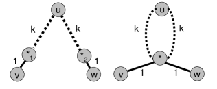
Figure 2: Due to the lack of a trace between $v$ and $w$, the stretch of an inferred topology can be large.

Lemma 3.14.

Let $u$ and $v$ be two arbitrary named nodes in the connected topologies $G_{1}$ and $G_{2}$. Then, even for only two stars in the trace set, it holds for the stretch that $\rho\leq(N-1)/2$. There are instances $G_{1},G_{2}$ that reach this bound.

We now turn our attention to the diameter and the degree.

Lemma 3.15.

For connected topologies $G_{1},G_{2}$ it holds that $\textsc{Diam}(G_{1})-\textsc{Diam}(G_{2})\leq(s-1)/s\cdot\textsc{Diam}(G_{C})\leq(s-1)(N-1)/s$ and $\textsc{Diam}(G_{1})/\textsc{Diam}(G_{2})\leq s$, where Diam denotes the graph diameter and $\textsc{Diam}(G_{1})>\textsc{Diam}(G_{2})$. There are instances $G_{1},G_{2}$ that reach these bounds.

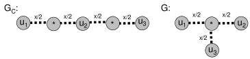
Figure 3: Estimation error for diameter.

Proof.

Upper bound: As $G_{C}$ does not merge any stars, it describes the network with the largest diameter. Let $\pi$ be a longest path between two nodes $u$ and $v$ in $G_{C}$. In the extreme case, $\pi$ is the only path determining the network diameter and $\pi$ contains all star nodes. Then, the graph where all $s$ stars are merged into one anonymous node has a minimal diameter of at least $\textsc{Diam}(G_{C})/s$.

Example meeting the bound: Consider the trace set $\mathcal{T}$ $=\{(u_{1},\ldots,*_{1},\ldots,u_{2}),$ $(u_{2},\ldots,*_{2},\ldots,u_{3}),$ $\ldots,$ $(u_{s},\ldots,*_{s},$ $\ldots,u_{s+1})\}$ with $x$ named nodes and star in the middle between $u_{i}$ and $u_{i+1}$ (assume $x$ to be even, $x$ does not include $u_{i}$ and $u_{i+1}$ ). It holds that $\textsc{Diam}(G_{C})=s\cdot(x+2)$ whereas in a graph $G$ where all stars are merged, $\textsc{Diam}(G)=x+2$. There are $n=s(x+1)$ non-anonymous nodes, so $x=(n-s-1)/s$. Figure 3 depicts an example. ∎

Lemma 3.16.

For the maximal node degree Deg, we have $\textsc{Deg}(G_{1})-\textsc{Deg}(G_{2})\leq 2(s-\gamma(G_{*}))$ and $\textsc{Deg}(G_{1})/\textsc{Deg}(G_{2})\leq s-\gamma(G_{*})+1$. There are instances $G_{1},G_{2}$ that reach these bounds.

Another important topology measure that indicates how well meshed the network is, is the number of triangles.

Lemma 3.17.

Let $C_{3}(G)$ be the number of cycles of length $3$ of the graph $G$. It holds that $C_{3}(G_{1})-C_{3}(G_{2})\leq 2s(s-1)$, which can be reached. The relative error $C_{3}(G_{1})/C_{3}(G_{2})$ can be arbitrarily large unless the number of links between non-anonymous nodes exceeds $n^{2}/4$ in which case the ratio is upper bounded by $2s(s-1)+1$.

Proof.

Upper bound: Each node which is part of a triangle has at least two incident edges. Thus, a node $v$ can be part of at most $\textsc{Deg}(v)\choose 2$ triangles, where $\textsc{Deg}(v)$ denotes $v$’s degree. As a consequence the number of triangles containing an anonymous node in an inferrable topology with $a$ anonymous nodes $u_{1},\ldots u_{a}$ is at most $\sum_{j=1}^{a}$ $\textsc{Deg}(u_{j})\choose 2$. Given $s$, this sum is maximized if $a=1$ and $\textsc{Deg}(u_{1})=2s$ as $2s$ is the maximum degree possible due to Lemma 3.16. Thus there can be at most $s\cdot(2s-1)$ triangles containing an anonymous node in $G_{1}$. The number of triangles with at least one anonymous node is minimized in $G_{C}$ because in the canonic graph the degrees of the anonymous nodes are minimized, i.e, they are always exactly two. As a consequence there cannot be more than $s$ such triangles in $G_{C}$.

If the number of such triangles in $G_{C}$ is smaller by $x$, then the number of of triangles with at least one anonymous node in the topology $G_{1}$ is upper bounded by $s\cdot(2s-1)-x$. The difference between the triangles in $G_{1}$ and $G_{2}$ is thus at most $s(2s-1)-x-s+x=2s(s-1)$.

Example meeting this bound: If the non-anonymous nodes form a complete graph and all star nodes can be merged into one node in $G_{1}$ and $G_{2}=G_{C}$, then the difference in the number of triangles matches the upper bound. Consequently it holds for the ratio of triangles with anonymous nodes that it does not exceed $(s(2s-1)-x)/(s-x).$ Thus the ratio can be infinite, as $x$ can reach $s$. However, if the number of links between $n$ non-anonymous nodes exceeds $n^{2}/4$ then there is at least one triangle, as the densest complete bipartite graph contains at most $n^{2}/4$ links. ∎

4 Full Exploration

So far, we assumed that the trace set $\mathcal{T}$ contains each node and link of $G_{0}$ at least once. At first sight, this seems to be the best we can hope for. However, sometimes traces exploring the vicinity of anonymous nodes in different ways yields additional information that help to characterize $\mathcal{G}_{\mathcal{T}}$ better.

This section introduces the concept of fully explored networks: $\mathcal{T}$ contains sufficiently many traces such that the distances between non-anonymous nodes can be estimated accurately.

Definition 4.1 (Fully Explored Topologies).

A topology $G_{0}$ is fully explored by a trace set $\mathcal{T}$ if it contains all nodes and links of $G_{0}$ and for each pair $\{u,v\}$ of non-anonymous nodes in the same component of $G_{0}$ there exists a trace $T\in\mathcal{T}$ containing both nodes $u\in T$ and $v\in T$.

In some sense, a trace set for a fully explored network is the best we can hope for. Properties that cannot be inferred well under the fully explored topology model are infeasible to infer without additional assumptions on $G_{0}$. In this sense, this section provides upper bounds on what can be learned from topology inference. In the following, we will constrain ourselves to routing along shortest paths only ($\alpha=1$).

Let us again study the properties of the family of inferrable topologies fully explored by a trace set. Obviously, all the upper bounds from Section 3 are still valid for fully explored topologies. In the following, let $G_{1},G_{2}\in\mathcal{G}_{\mathcal{T}}$ be arbitrary representatives of $\mathcal{G}_{\mathcal{T}}$ for a fully explored trace set $\mathcal{T}$. A direct consequence of the Definition 4.1 concerns the number of connected components and the stretch. (Recall that the stretch is defined with respect to named nodes only, and since $\alpha=1$, a 1-consistent inferrable topology cannot include a shorter path between $u$ and $v$ than the one that must appear in a trace of $\mathcal{T}$.)

Lemma 4.2.

It holds that $\textsc{Comp}(G_{1})=\textsc{Comp}(G_{2})$ ($=\textsc{Comp}(G_{0})$) and the stretch is 1.

The proof for the claims of the following lemmata are analogous to our former proofs, as the main difference is the fact that there might be more conflicts, i.e., edges in $G_{*}$.

Lemma 4.3.

For fully explored networks it holds that $|V_{1}|-|V_{2}|\leq s-\gamma(G_{*})\leq s-1$ and $|V_{1}|/|V_{2}|\leq(n+s)/(n+\gamma(G_{*}))\leq(2+s)/3$. Moreover, $|E_{1}|-|E_{2}|\in 2(s-\gamma(G_{*}))$ and $|E_{1}|/|E_{2}|\leq(\nu+2s)/(\nu+2)\leq s$, where $\nu$ denotes the number of links between non-anonymous nodes. There are traces with inferrable topology $G_{1},G_{2}$ reaching these bounds.

Lemma 4.4.

For the maximal node degree, we have $\textsc{Deg}(G_{1})-\textsc{Deg}(G_{2})\leq 2(s-\gamma(G_{*}))$ and $\textsc{Deg}(G_{1})/\textsc{Deg}(G_{2})\leq s-\gamma(G_{*})+1$. There are instances $G_{1},G_{2}$ that reach these bounds.

From Lemma 4.2 we know that fully explored scenarios yield a perfect stretch of one. However, regarding the diameter, the situation is different in the sense that distances between anonymous nodes play a role.

Lemma 4.5.

For connected topologies $G_{1},G_{2}$ it holds that $\textsc{Diam}(G_{1})/\textsc{Diam}(G_{2})\leq 2$, where Diam denotes the graph diameter and $\textsc{Diam}(G_{1})>\textsc{Diam}(G_{2})$. There are instances $G_{1},G_{2}$ that reach this bound. Moreover, there are instances with $\textsc{Diam}(G_{1})-\textsc{Diam}(G_{2})=s/2$.

The number of triangles with anonymous nodes can still not be estimated accurately in the fully explored scenario.

Lemma 4.6.

There exist graphs where $C_{3}(G_{1})-C_{3}(G_{2})=s(s-1)/2$, and the relative error $C_{3}(G_{1})/C_{3}(G_{2})$ can be arbitrarily large.

5 Conclusion

We understand our work as a first step to shed light onto the similarity of inferrable topologies based on most basic axioms and without any assumptions on power-law properties, i.e., in the worst case. Using our formal framework we show that the topologies for a given trace set may differ significantly. Thus, it is impossible to accurately characterize topological properties of complex networks. To complement the general analysis, we propose the notion of fully explored networks or trace sets, as a “best possible scenario”. As expected, we find that fully exploring traces allow us to determine several properties of the network more accurately; however, it also turns out that even in this scenario, other topological properties are inherently hard to compute. Our results are summarized in Figure 4.

Property/Scenario	Arbitrary		Fully Explored ($\alpha=1$)
	$G_{1}-G_{2}$	$G_{1}/G_{2}$	$G_{1}-G_{2}$	$G_{1}/G_{2}$
# of nodes	$\leq s-\gamma(G_{*})$	$\leq(n+s)/(n+\gamma(G_{*}))$	$\leq s-\gamma(G_{*})$	$\leq(n+s)/(n+\gamma(G_{*}))$
# of links	$\leq 2(s-\gamma(G_{*}))$	$\leq(\nu+2s)/(\nu+2)$	$\leq 2(s-\gamma(G_{*}))$	$\leq(\nu+2s)/(\nu+2)$
# of connected components	$\leq n/2$	$\leq n/2$	$=0$	$=1$
Stretch	-	$\leq(N-1)/2$	-	$=1$
Diameter	$\leq(s-1)/s\cdot(N-1)$	$\leq s$	$s/2$ ($\P$)	$2$
Max. Deg.	$\leq 2(s-\gamma(G_{*}))$	$\leq s-\gamma(G_{*})+1$	$\leq 2(s-\gamma(G_{*}))$	$\leq s-\gamma(G_{*})+1$
Triangles	$\leq 2s(s-1)$	$\infty$	$\leq 2s(s-1)/2$	$\infty$

Figure 4: Summary of our bounds on the properties of inferrable topologies. $s$ denotes the number of stars in the traces, $n$ is the number of named nodes, $N=n+s$, and $\nu$ denotes the number of links between named nodes. Note that trace sets meeting these bounds exist for all properties for which we have tight or upper bounds. For the two entries marked with ($\P$), only “lower bounds” are derived, i.e., examples that yield at least the corresponding accuracy; as the upper bounds from the arbitrary scenario do not match, how to close the gap remains an open question.

Our work opens several directions for future research. On a theoretical side, one may study whether the minimal inferrable topologies considered in, e.g., [1, 2], are more similar in nature. More importantly, while this paper presented results for the general worst-case, it would be interesting to devise algorithms that compute, for a given trace set, worst-case bounds for the properties under consideration. For example, such approximate bounds would be helpful to decide whether additional measurements are needed. Moreover, maybe such algorithms may even give advice on the locations at which such measurements would be most useful.

Appendix A Deferred Proofs

A.1 Proof of Theorem 3.2

Fix $\mathcal{T}$. We have to prove that $G_{C}$ fulfills Axiom 0, Axiom 1 (which implies Axiom 3) and Axiom 2.

Axiom 0: The axiom holds trivially: only edges from the traces are used in $G_{C}$.

Axiom 1: Let $T\in\mathcal{T}$ and $\sigma_{1},\sigma_{2}\in T$. Let $k=d_{T}(\sigma_{1},\sigma_{2})$. We show that $G_{C}$ fulfills Axiom 1, namely, there exists a path of length $k$ in $G_{C}$. Induction on $k$: ($k=1$:) By the definition of $G_{C}$, $\{\sigma_{1},\sigma_{2}\}\in E_{C}$ thus there exists a path of length one between $\sigma_{1}$ and $\sigma_{2}$. ($k>1$:) Suppose Axiom 1 holds up to $k-1$. Let $\sigma^{\prime}_{1},\ldots,\sigma^{\prime}_{k-1}$ be the intermediary nodes between $\sigma_{1}$ and $\sigma_{2}$ in $T$: $T=(\ldots,\sigma_{1},\sigma^{\prime}_{1},\ldots,\sigma^{\prime}_{k-1},\sigma_{2},\ldots)$. By the induction hypothesis, in $G_{C}$ there is a path of length $k-1$ between $\sigma_{1}$ and $\sigma^{\prime}_{k-1}$. Let $\pi$ be this path. By definition of $G_{C}$, $\{\sigma^{\prime}_{k-1},\sigma_{2}\}\in E_{C}$. Thus appending $(\sigma^{\prime}_{k-1},\sigma_{2})$ to $\pi$ yields the desired path of length $k$ linking $\sigma_{1}$ and $\sigma_{2}$: Axiom 1 thus holds up to $k$.

Axiom 2: We have to show that $d_{T}(\sigma_{1},\sigma_{2})=k\Rightarrow d_{C}(\sigma_{1},\sigma_{2})\geq\lceil\alpha\cdot k\rceil$. By contradiction, suppose that $G_{C}$ does not fulfill Axiom 2 with respect to $\alpha$. So there exists $k^{\prime}<\lceil\alpha\cdot k\rceil$ and $\sigma_{1},\sigma_{2}\in V_{C}$ such that $d_{C}(\sigma_{1},\sigma_{2})=k^{\prime}$. Let $\pi$ be a shortest path between $\sigma_{1}$ and $\sigma_{2}$ in $G_{C}$. Let $(T_{1},\ldots,T_{\ell})$ be the corresponding (maybe repeating) traces covering this path $\pi$ in $G_{C}$. Let $T_{i}\in(T_{1},\ldots,T_{\ell})$, and let $s_{i}$ and $e_{i}$ be the corresponding start and end nodes of $\pi$ in $T_{i}$. We will show that this path $\pi$ implies the existence of a path in $G_{0}$ which violates $\alpha$-consistency. Since $G_{0}$ is inferrable, $G_{0}$ fulfills Axiom 2, thus we have: $d_{C}(\sigma_{1},\sigma_{2})=\sum_{i=1}^{\ell}d_{T_{i}}(s_{i},e_{i})=k^{\prime}<\lceil\alpha\cdot k\rceil\leq d_{G_{0}}(\sigma_{1},\sigma_{2})$ since $G_{0}$ is $\alpha$-consistent. However, $G_{0}$ also fulfills Axiom 1, thus $d_{T_{i}}(s_{i},e_{i})\geq d_{G_{0}}(s_{i},e_{i})$. Thus $\sum_{i=1}^{\ell}d_{G_{0}}(s_{i},e_{i})\leq\sum_{i=1}^{\ell}d_{T_{i}}(s_{i},e_{i})<d_{G_{0}}(\sigma_{1},\sigma_{2})$: we have constructed a path from $\sigma_{1}$ to $\sigma_{2}$ in $G_{0}$ whose length is shorter than the distance between $\sigma_{1}$ and $\sigma_{2}$ in $G_{0}$, leading to the desired contradiction.

A.2 Proof of Lemma 3.5

First we construct a topology $G_{0}=(V_{0},E_{0})$ and then describe a trace set on this graph that generates the star graph $G=(V,E)$. The node set $V_{0}$ consists of $|V|$ anonymous nodes and $|V|\cdot(1+\tau)$ named nodes, where $\tau=\lceil 3/(2\alpha)-1/2\rceil$. The first building block of $G_{0}$ is a copy of $G$. To each node $v_{i}$ in the copy of $G$ we add a chain consisting of $2+\tau$ nodes, first appending $\tau$ non-anonymous nodes $w_{(i,k)}$ where $1\leq k\leq\tau$, followed by an anonymous node $u_{i}$ and finally a named node $w_{(i,\tau+1)}$. More formally we can describe the link set as $E_{0}=E\cup\bigcup_{i=1}^{|V|}\left(\{v_{i},w_{(i,1)}\},\{w_{(i,1)},w_{(i,2)}\},\ldots,\{w_{(i,\tau)},u_{i}\},\{u_{i},w_{(i,\tau+1)}\}\right)$. The trace set $\mathcal{T}$ consists of the following $|V|+|E|$ shortest path traces: the traces $T_{\ell}$ for $\ell\in\{1,\ldots,|V|\}$, are given by $T_{\ell}(w_{(\ell,\tau)},w_{(\ell,\tau+1)})$ (for each node in $V$), and the traces $T_{\ell}$ for ${\ell}\in\{|V|+1,\ldots,|V|+|E|\}$, are given by $T_{\ell}(w_{(i,\tau)},w_{(j,\tau)})$ for each link $\{v_{i},v_{j}\}$ in $E$. Note that $G_{0}=G_{C}$ as each star appears as a separate anonymous node. The star graph $G_{*}$ corresponding to this trace set contains the $|V|$ nodes $*_{i}$ (corresponding to $u_{i}$). In order to prove the claim of the lemma we have to show that two nodes $*_{i},*_{j}$ are conflicting according to Lemma 3.3 if and only if there is a link $\{v_{i},v_{j}\}$ in $E$. Case $(i)$ does not apply because the minimum distance between any two nodes in the canonic graph is at least one, and $\lceil\alpha\cdot d_{T_{i}}(*_{i},w_{(i,\tau)})\rceil=1$ and $\lceil\alpha\cdot d_{T_{i}}(*_{i},w_{(i,\tau+1)})\rceil=1$. It remains to examine Case $(ii)$: “$\Rightarrow$” if $\textsc{Map}(*_{i})=\textsc{Map}(*_{j})$ there would be a path of length two between $w_{(i,\tau)}$ and $w_{(j,\tau)}$ in the topology generated by Map; the trace set however contains a trace $T_{\ell}(w_{(i,\tau)},w_{(j,\tau)})$ of length $2\tau+1$. So $\lceil\alpha\cdot d_{T_{\ell}}(w_{(i,\tau)},w_{(j,\tau)})\rceil=\lceil\alpha\cdot(2\tau+1)\rceil=\lceil\alpha\cdot(2\lceil 3/(2\alpha)-1/2\rceil+1\rceil)\geq 3$, which violates the $\alpha$-consistency (Lemma 3.3 (ii)) and hence $\{*_{i},*_{j}\}\in E_{*}$ and $\{v_{i},v_{j}\}\in E$. “$\Leftarrow$”: if $\{v_{i},v_{j}\}\not\in E$, there is no trace $T(w_{(i,\tau)},w_{(j,\tau)})$, thus we have to prove that no trace $T_{\ell}(w_{(i^{\prime},\tau)},w_{(j^{\prime},\tau)})$ with $i^{\prime}\neq i$ and $j^{\prime}\neq j$ and $j^{\prime}\neq i$ leads to a conflict between $*_{i}$ and $*_{j}$. We show that an even more general statement is true, namely that for any pair of distinct non-anonymous nodes $x_{1},x_{2}$, where $x_{1},x_{2}\in\{v_{i^{\prime}},v_{j^{\prime}},w_{(i^{\prime},k)},w_{(j^{\prime},k)}|1\leq k\leq\tau+1,i^{\prime}\neq i,j^{\prime}\neq i,j^{\prime}\neq j\}$, it holds that $\lceil\alpha\cdot d_{C}(x_{1},x_{2})\rceil\leq d_{C}(x_{1},*_{i})+d_{C}(x_{2},*_{j})$. Since $G_{C}=G_{0}$ and the traces contain shortest paths only, the trace distance between two nodes in the same trace is the same as the distance in $G_{C}$. The following tables contain the relevant lower bounds on distances in $G_{C}$ and $\mu(x_{1},x_{2})=d_{C}(x_{1},*_{i})+d_{C}(x_{2},*_{j})$.

$d_{C}(\cdot,\cdot)\geq$	$v_{i^{\prime}}$	$v_{j^{\prime}}$	$w_{(i^{\prime},k_{1})}$	$w_{(j^{\prime},k_{1})}$
$v_{i^{\prime}}$	0	1	$k_{1}$	$k_{1}+1$
$v_{j^{\prime}}$	1	0	$k_{1}$ + 1	$k_{1}$
$w_{(i^{\prime},k_{2})}$	$k_{2}$	$k_{2}+1$	$|k_{2}-k_{1}|$	$k_{1}+1+k_{2}$
$w_{(j^{\prime},k_{2})}$	$k_{2}+1$	$k_{2}$	$k_{1}+1+k_{2}$	$|k_{2}-k_{1}|$
$*_{i}$	$\tau+2$	$\tau+1$	$2+\tau+k_{1}$	$\tau-k_{1}+1$
$*_{j}$	$\tau+2$	$\tau+2$	$2+\tau+k_{1}$	$2+\tau+k_{1}$
$\mu(\cdot,\cdot)\geq$	$v_{i^{\prime}}$	$v_{j^{\prime}}$	$w_{(i^{\prime},k_{1})}$	$w_{(j^{\prime},k_{1})}$
$v_{i^{\prime}}$	$2\tau+4$	$2\tau+3$	$4+2\tau+k_{1}$	$4+2\tau+k_{1}$
$v_{j^{\prime}}$	$2\tau+3$	$2\tau+4$	$2\tau+3+k_{1}$	$3+2\tau+k_{1}$
$w_{(i^{\prime},k_{2})}$	$4+2\tau+k_{2}$	$4+2\tau+k_{2}$	$4+2\tau+k_{1}+k_{2}$	$4+2\tau+k_{1}+k_{2}$
$w_{(j^{\prime},k_{2})}$	$2\tau-k_{2}+3$	$2\tau-k_{2}+3$	$2\tau+3+k_{1}-k_{2}$	$2\tau+k_{1}-k_{2}+3$

Table 1: Proof of Lemma 3.5: lower bounds for the distances in $G_{C}$, and lower bounds for $\mu(x_{1},x_{2})=d_{C}(x_{1},*_{i})+d_{C}(x_{2},*_{j})$.

If $x_{1}\neq w_{(j^{\prime},k_{2})}$ then it holds for all $x_{1},x_{2}$ that $d_{T_{\ell}}(x_{1},x_{2})\leq 2\tau+1$ whereas $\mu(x_{1},x_{2})=d_{C}(x_{1},*_{i})+d_{C}(x_{2},*_{j})\geq 2\tau+2$. In all other cases it holds at least that $d_{C}(x_{1},x_{2})<\mu(x_{1},x_{2})$. Thus $\lceil\alpha\cdot d_{C}(x_{1},x_{2})\rceil\leq d_{C}(x_{1},*_{i})+d_{C}(x_{2},*_{j})$. Consequently, we have conflicts if and only if $\{v_{i},v_{j}\}\in E$, which concludes the proof.

A.3 Proof of Lemma 3.7

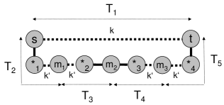
Figure 5: Visualization for proof of Lemma 3.7. Solid lines denote links, dashed lines denote paths (of annotated length).

We have to show that the paths in the traces correspond to paths in $G_{\gamma}$. Let $T\in\mathcal{T}$, and $\sigma_{1},\sigma_{2}\in T$. Let $\pi$ be the sequence of nodes in $T$ connecting $\sigma_{1}$ and $\sigma_{2}$. This is also a path in $G_{\gamma}$: since $\alpha>0$, for any two symbols $\sigma_{1},\sigma_{2}\in T$, it holds that $\textsc{Map}(\sigma_{1})\neq\textsc{Map}(\sigma_{2})$ as $\alpha>0$.

We now construct an example showing that the $\alpha^{\prime}$ for which $G_{\gamma}$ fulfills Axiom 2 can be arbitrarily small. Consider the graph represented in Figure 5. Let $T_{1}=(s,\ldots,t),T_{2}=(s,*_{1},\ldots,m_{1}),T_{3}=(m_{1},\ldots,*_{2},m_{2}),T_{4}=(m_{2},*_{3},\ldots,m_{3}),T_{5}=(m_{3},\ldots,*_{4},t)$. We assume $\alpha=1$. By changing parameters $k=d_{C}(s,t)$ and $k^{\prime}=d_{C}(m_{1},*_{1})=d_{C}(m_{1},*_{2})=d_{C}(m_{3},*_{3})=d_{C}(m_{3},*_{4})$, we can modulate the links of the corresponding star graph $G_{*}$. Using $d_{T_{1}}(s,t)=k$, observe that $k>2\Leftrightarrow\{*_{1},*_{4}\}\in E_{*}$. Similarly, $k>2(k^{\prime}+1)\Leftrightarrow\{*_{1},*_{3}\}\in E_{*}\wedge\{*_{2},*_{4}\}\in E_{*}$ and $k>2(k^{\prime}+2)\Leftrightarrow\{*_{1},*_{2}\}\in E_{*}\wedge\{*_{3},*_{4}\}\in E_{*}$. Taking $k=2k^{\prime}+4$, we thus have $E_{*}=\{\{*_{1},*_{3}\},\{*_{2},*_{4}\},\{*_{1},*_{4}\}\}$.

Thus, we here construct a situation where $*_{1}$ and $*_{2}$ as well as $*_{3}$ and $*_{4}$ can be merged without breaking the consistency requirement, but where merging both simultaneously leads to a topology $G^{\prime}$ that is only $4/k$-consistent, since $d_{G^{\prime}}(s,t)=4$. This ratio can be made arbitrarily small provided we choose $k^{\prime}=(k-4)/2$.

A.4 Proof of Lemma 3.11

In the worst-case, each star in the trace represents a different node in $G_{1}$, so the maximal number of nodes in any topology in $\mathcal{G}_{\mathcal{T}}$ is the total number of non-anonymous nodes plus the total number of stars in $\mathcal{T}$. This number of nodes is reached in the topology $G_{C}$. According to Definition 3.4, only non-adjacent stars in $G_{*}$ can represent the same node in an inferrable topology. Thus, the stars in trace $\mathcal{T}$ must originate from at least $\gamma(G_{*})$ different nodes. As a consequence $|V_{1}|-|V_{2}|\leq s-\gamma(G_{*})$, which can reach $s-1$ for a trace set $\mathcal{T}=\{T_{i}=(v,*_{i},w)|1\leq i\leq s\}$. Analogously, $|V_{1}|/|V_{2}|\leq(n+s)/(n+\gamma(G_{*}))\leq(2+s)/3$.

Observe that each occurrence of a node in a trace describes at most two edges. If all anonymous nodes are merged into $\gamma(G_{*})$ nodes in $G_{1}$ and are separate nodes in $G_{2}$ the difference in the number of edges is at most $2(s-\gamma(G_{*}))$. Analogously, $|E_{1}|/|E_{2}|\leq(\nu+2s)/(\nu+2)\leq s$. The trace set $\mathcal{T}=\{T_{i}=(v,*_{i},w)|1\leq i\leq s\}$ reaches this bound.

A.5 Proof of Lemma 3.14

An “lower bound” example follows from Figure 2. Essentially, this is also the worst case: note that the difference in the shortest distance between a pair of nodes $u$ and $v$ in $G_{1}$ and $G_{2}$ is only greater than 0 if the shortest path between them involves at least one anonymous node. Hence the shortest distance between such a pair is two. The longest shortest distance between the same pair of nodes in another inferred topology visits all nodes in the network, i.e., its length is bounded by $N-1$.

A.6 Proof of Lemma 3.16

Each occurrence of a node in a trace describes at most two links incident to this node. For the degree difference we only have to consider the links incident to at least one anonymous node, as the number of links between non-anonymous nodes is the same in $G_{1}$ and $G_{2}$. If all anonymous nodes can be merged into $\gamma(G_{*})$ nodes in $G_{1}$ and all anonymous nodes are separate in $G_{2}$ the difference in the maximum degree is thus at most $2(s-\gamma(G_{*}))$, as there can be at most $s-\gamma(G_{*})+1$ nodes merged into one node and the minimal maximum degree of a node in $G_{2}$ is two. This bound is tight, as the trace set $T_{i}=\{v_{i},*,w_{i}\}$ for $1\leq i\leq s$ containing $s$ stars can be represented by a graph with one anonymous node of degree $2s$ or by a graph with $s$ anonymous nodes of degree two each. For the ratio of the maximal degree we can ignore links between non-anonymous nodes as well, as these only decrease the ratio. The highest number of links incident at node $v$ with one endpoint in the set of anonymous nodes is $s-\gamma(G_{*})+1$ for non-anonymous nodes and $2(s-\gamma(G_{*})+1)$ for anonymous nodes, whereas the lowest number is two.

A.7 Proof of Lemma 4.4

The proof for the upper bound is analogous to the case without full exploration. To prove that this bound can be reached, we need to add traces to the trace set to ensure that all pairs of named nodes appear in the trace but does not change the degrees of anonymous nodes. To this end we add a named node $u$ for each pair $\{v,w\}$ that is not in the trace set yet to $G_{0}$ and a trace $T=\{v,u,w\}$. This does not increase the maximum degree and guarantees full exploration.

A.8 Proof of Lemma 4.5

We first prove the upper bound for the relative case. Note that the maximal distance between two anonymous nodes $\textsc{Map}(*_{1})$ and $\textsc{Map}(*_{2})$ in an inferred topology component cannot be larger than twice the distance of two named nodes $u$ and $v$: from Definition 4.1 we know that there must be a trace in $\mathcal{T}$ connecting $u$ and $v$, and the maximal distance $\delta$ of a pair of named nodes is given by the path of the trace that includes $u$ and $v$. Therefore, and since any trace starts and ends with a named node, any star can be at a distance at a distance $\delta/2$ from a named node. Therefore, the maximal distance between $\textsc{Map}(*_{1})$ and $\textsc{Map}(*_{2})$ is $\delta/2+\delta/2$ to get to the corresponding closest named nodes, plus $\delta$ for the connection between the named nodes. As according to Lemma 4.2, the distance between named nodes is the same in all inferred topologies, the diameter of inferred topologies can vary at most by a factor of two.

We now construct an example that reaches this bound. Consider a topology consisting of a center node $c$ and four rays of length $k$. Let $u_{1},u_{2},u_{3},u_{4}$ be the “end nodes” of each ray. We assume that all these nodes are named. Now add two chains of anonymous nodes of length $2k+1$ between nodes $u_{1}$ and $u_{2}$, and between nodes $u_{3}$ and $u_{4}$ to the topology. The trace set consists of the minimal trace set to obtain a fully explored topology: six traces of length $2k+1$ between each pair of end nodes $u_{1},u_{2},u_{3},u_{4}$. Now we add two traces of length $2k+1$ between nodes $u_{1}$ and $u_{2}$, and between nodes $u_{3}$ and $u_{4}$. These traces explore the anonymous chains and have the following shape: $T_{7}=(u_{1},*_{1},\ldots,*_{k},\sigma,*_{k+1},\ldots,*_{2k},u_{2})$ and $T_{8}=(u_{3},*_{2k+1},\ldots,*_{3k},\sigma^{\prime},*_{3k+1},\ldots,*_{4k},u_{4})$, where $\sigma$ and $\sigma^{\prime}$ are stars. Let $G_{1}=G_{C}$ and $G_{2}$ be the inferrable graph where $\sigma$ and $\sigma^{\prime}$ are merged. The resulting diameters are $\textsc{Diam}(G_{1})=4k+2$ and $\textsc{Diam}(G_{2})=2k+1$. Since $s=4k+2$, the difference can thus be as large as $s/2$. Note that this construction also yields the bound of the relative difference: $\textsc{Diam}(G_{1})/\textsc{Diam}(G_{2})=(4k+2)/(2k+1)=2$.

A.9 Proof of Lemma 4.6

Given the number of stars $s$, we construct a trace set $\mathcal{T}$ with two inferrable graphs such that in one graph the number of triangles with anonymous nodes is $s(s-1)/2$ and in the other graph there are no such triangles. As a first step we add $s$ traces $T_{i}=(v_{i},*_{i},w)$ to the trace set $\mathcal{T}$, where $1\leq i\leq s$. To make this trace set fully explored we add traces for each pair $v_{i},v_{j}$ to $\mathcal{T}$ as a second step, i.e., traces $T_{i,j}=(v_{i},v_{j})$ for $1\leq i\leq s$ and $1\leq j\leq s$. The resulting trace set contains $s$ stars and none of the stars are in conflict with each other. Thus the graph $G_{1}$ merging all stars into one anonymous node is inferrable from this trace and the number of triangles where the anonymous node is part of is $s(s-1)/2$. Let $G_{2}$ be the canonic graph of this trace set. This graph does not contain any triangles with anonymous nodes and hence the difference $C(G_{1})-C(G_{2})$ is $s(s-1)/2$.

To see that the ratio can be unbounded look at the trace set $\{(v,*_{1},w),(u,*_{2},w),(u,v)\}$. This set is fully explored since all pairs of named nodes appear in a trace. The graph where the two stars are merged has one triangle and the canonic graph has no triangle.

References

- [1] H. Acharya and M. Gouda. The weak network tracing problem. In Proc. Int. Conference on Distributed Computing and Networking (ICDCN), pages 184–194, 2010.
- [2] H. Acharya and M. Gouda. On the hardness of topology inference. In Proc. Int. Conference on Distributed Computing and Networking (ICDCN), pages 251–262, 2011.
- [3] Hrishikesh B. Acharya and Mohamed G. Gouda. A theory of network tracing. In Proc. 11th International Symposium on Stabilization, Safety, and Security of Distributed Systems (SSS), pages 62–74, 2009.
- [4] Animashree Anandkumar, Avinatan Hassidim, and Jonathan Kelner. Topology discovery of sparse random graphs with few participants. In Proc. SIGMETRICS, 2011.
- [5] Brice Augustin, Xavier Cuvellier, Benjamin Orgogozo, Fabien Viger, Timur Friedman, Matthieu Latapy, Clémence Magnien, and Renata Teixeira. Avoiding traceroute anomalies with paris traceroute. In Proc. 6th ACM SIGCOMM Conference on Internet Measurement (IMC), pages 153–158, 2006.
- [6] Mark Buchanan. Data-bots chart the internet. Science, 813(3), 2005.
- [7] Bill Cheswick, Hal Burch, and Steve Branigan. Mapping and visualizing the internet. In Proc. USENIX Annual Technical Conference (ATEC), 2000.
- [8] Michalis Faloutsos, Petros Faloutsos, and Christos Faloutsos. On power-law relationships of the internet topology. In Proc. SIGCOMM, pages 251–262, 1999.
- [9] M. Gunes and K. Sarac. Resolving anonymous routers in internet topology measurement studies. In Proc. INFOCOM, 2008.
- [10] Xing Jin, W.-P.K. Yiu, S.-H.G. Chan, and Yajun Wang. Network topology inference based on end-to-end measurements. IEEE Journal on Selected Areas in Communications, 24(12):2182 –2195, 2006.
- [11] Craig Labovitz, Abha Ahuja, Srinivasan Venkatachary, and Roger Wattenhofer. The impact of internet policy and topology on delayed routing convergence. In Proc. 20th Annual Joint Conference of the IEEE Computer and Communications Societies (INFOCOM), 2001.
- [12] S. Paul, K. K. Sabnani, J. C. Lin, and S. Bhattacharyya. Reliable multicast transport protocol (rmtp). IEEE Journal on Selected Areas in Communications, 5(3), 1997.
- [13] Ingmar Poese, Benjamin Frank, Bernhard Ager, Georgios Smaragdakis, and Anja Feldmann. Improving content delivery using provider-aided distance information. In Proc. ACM IMC, 2010.
- [14] H. Tangmunarunkit, R. Govindan, S. Shenker, and D. Estrin. The impact of routing policy on internet paths. In Proc. INFOCOM, volume 2, pages 736–742, 2002.
- [15] Bin Yao, Ramesh Viswanathan, Fangzhe Chang, and Daniel Waddington. Topology inference in the presence of anonymous routers. In Proc. IEEE INFOCOM, pages 353–363, 2003.