Fabian Scheipl spikeSlabGAM: Bayesian Variable Selection, Model Choice and Regularization for Generalized Additive Mixed Models in R spikeSlabGAM: Variable Selection and Model Choice for GAMMs The R package spikeSlabGAM implements Bayesian variable selection, model choice, and regularized estimation in (geo-)additive mixed models for Gaussian, binomial, and Poisson responses. Its purpose is to (1) choose an appropriate subset of potential covariates and their interactions, (2) to determine whether linear or more flexible functional forms are required to model the effects of the respective covariates, and (3) to estimate their shapes. Selection and regularization of the model terms is based on a novel spike-and-slab-type prior on coefficient groups associated with parametric and semi-parametric effects. MCMC, P-splines, spike-and-slab prior, normal-inverse-gamma MCMC, P-splines, spike-and-slab prior, normal-inverse-gamma Fabian Scheipl
Institut für Statistik
LMU München
Ludwigstr. 33
80539 München, Germany
E-mail:
URL: http:/www.stat.uni-muenchen.de/~scheipl/

spikeSlabGAM: Bayesian Variable Selection, Model Choice and Regularization for Generalized Additive Mixed Models in R

1 Introduction

In data sets with many potential predictors, choosing an appropriate subset of covariates and their interactions at the same time as determining whether linear or more flexible functional forms are required to model the relationships between covariates and the response is a challenging and important task. From a Bayesian perspective, it can be translated into a question of estimating marginal posterior probabilities of whether a variable should be in the model and in what form (i.e., linear or smooth; as a main effect and/or as an effect modifier).

We introduce the R (R Development Core Team, 2010) package spikeSlabGAM which implements fully Bayesian variable selection and model choice with a spike-and-slab prior structure that expands the approach in Ishwaran and Rao (2005) to select or deselect single coefficients as well as blocks of coefficients associated with specific model terms. The spike-and-slab priors we use are bimodal priors for the hyper-variances of the regression coefficients which result in a two component mixture of a narrow spike around zero and a slab with wide support for the marginal prior of the coefficients themselves. The posterior mixture weights for the spike component for a specific coefficient or coefficient batch can be interpreted as the posterior probability of its exclusion from the model.

The coefficient batches selected or deselected in this fashion can be associated with a wide variety of model terms such as simple linear terms, factor variables, basis expansions for the modeling of smooth curves or surfaces, intrinsically Gaussian Markov random fields (IGMRF), random effects, and all their interactions. spikeSlabGAM is able to deal with Gaussian, binomial and Poisson responses, and can be used to fit piecewise exponential models for time-to-event data. For these response types, the package presented here implements regularized estimation, term selection, model choice, and model averaging for a similarly broad class of models as that available in mboost (Hothorn et al., 2010) or BayesX (Brezger et al., 2005). To the best of our knowledge, it is the first implementation of a Bayesian model term selection method that: (1) is able to fit models for non-Gaussian responses from the exponential family; (2) selects and estimates many types of regularized effects with a (conditionally) Gaussian prior such as simple covariates (both metric and categorical), penalized splines (uni- or multivariate), random effects, spatial effects (kriging, IGMRF) and their interactions; (3) and can distinguish between smooth nonlinear and linear effects. The approach scales reasonably well to datasets with thousands of observations and a few hundred coefficients and is available in documented open source software.

Bayesian function selection, similar to the frequentist COSSO procedure (Lin and Zhang, 2006), is usually based on decomposing the additive model in the spirit of a smoothing spline ANOVA (Wahba et al., 1995). Wood et al. (2002) and Yau et al. (2003) describe procedures for Gaussian and latent Gaussian models using a data-based prior that requires two MCMC runs, a pilot run to obtain a data-based prior for the slab part and a second one to estimate parameters and select model components. A more general approach that also allows for flexible modeling of the dispersion in double exponential regression models is described in Cottet et al. (2008), but no implementation is available. Reich et al. (2009) also use the smoothing spline ANOVA framework and perform variable and function selection via SSVS for Gaussian responses. Frühwirth-Schnatter and Wagner (2010) discuss various spike-and-slab prior variants for the selection of random intercepts for Gaussian and latent Gaussian models.

The remainder of this paper is structured as follows: Section 2 gives some background on the two main ideas used in spikeSlabGAM. 2.1 introduces the necessary notation for the generalized additive mixed model and 2.2 fills in some details on the spike-and-slab prior. Section 3 relates details of the implementation: how the design matrices for the model terms are constructed (Section 3.1) and how the MCMC sampler works (Section 3.2). Section 4 explains how to specify, visualize and interpret models fitted with spikeSlabGAM and contains an application to the Pima Indian Diabetes dataset.

2 Background

2.1 Generalized additive mixed models

The generalized additive mixed model (GAMM) is a broad model class that forms a subset of structured additive regression (Fahrmeir et al., 2004). In a GAMM, the distribution of the responses $\bm{y}$ given a set of covariates $\bm{x}_{j}\;(j=1,\dots,p)$ belongs to an exponential family, i.e.,

$$\pi(y|x,\phi) =c(y,\phi)\exp\left(\frac{y\theta-b(\theta)}{\phi}\right),$$

with $\theta$,$\phi$,$b(\cdot)$ and $c(\cdot)$ determined by the type of distribution. The conditional expected value of the response $\operatorname{E}(\bm{y}|\bm{x}_{1},\ldots,\bm{x}_{p})=h(\bm{\eta})$ is determined by the additive predictor $\bm{\eta}$ and a fixed response function $h(\cdot)$.

The additive predictor

$$\bm{\eta} =\bm{\eta}_{o}+\bm{X}_{u}\bm{\beta}_{u}+\sum^{p}_{j=1}f_{j}(\bm{x})$$ (1)

has three parts: a fixed and known offset $\bm{\eta}_{o}$, a linear predictor $\bm{X}_{u}\bm{\beta}_{u}$ for model terms that are not under selection with coefficients $\bm{\beta}_{u}$ associated with a very flat Gaussian prior (this will typically include at least a global intercept term), and the model terms $f_{j}(\bm{x})=\left(f_{j}(\bm{x}_{1}),\ldots,f_{j}(\bm{x}_{n})\right)^{\top}\;(j=1,\dots,p)$ that are each represented as linear combinations of $d_{j}$ basis functions $B_{j}(\cdot)$ so that

$$\begin{split}f_{j}(\bm{x})&=\sum_{k=1}^{d_{j}}\beta_{jk}B_{jk}(\bm{x})=\bm{B}_{j}\bm{\beta}_{j},\text{ with }B_{jk}(\bm{x})=\left(B_{jk}(\bm{x}_{1}),\ldots,B_{jk}(\bm{x}_{n})^{\top}\right)\\ \text{ and }\bm{\beta}_{j}&\stackrel{{\scriptstyle\text{prior}}}{{\sim}}\operatorname{peNMIG}(v_{0},w,a_{\tau},b_{\tau})\text{ for }j=1,\dots,p.\end{split}$$ (2)

The peNMIG prior structure is explained in detail in Section 2.2.

Components $f_{j}(\bm{x})$ of the additive predictor represent a wide variety of model terms, such as (1) linear terms ($f_{j}(\bm{x})=\beta_{j}\bm{x}_{j}$), (2) nominal or ordinal covariates ($f(x_{ji})=\beta_{x(k)}$ iff $x_{ji}=k$, i.e., if entry $i$ in $\bm{x}_{j}$ is $k$), (3) smooth functions of (one or more) continuous covariates (splines, kriging effects, tensor product splines or varying coefficient terms, e.g., Wood (2006)), (4) Markov random fields for discrete spatial covariates (e.g. Rue and Held, 2005), (5) random effects (subject-specific intercepts or slope), and (6) interactions between the different terms (varying-coefficient models, effect modifiers, factor interactions). Estimates for semiparametric model terms and random effects are regularized in order to avoid overfitting and modeled with appropriate shrinkage priors. These shrinkage or regularization priors are usually Gaussian or can be parameterized as scale mixtures of Gaussians (e.g. Fahrmeir et al., 2010). The peNMIG variable selection prior used in spikeSlabGAM can also be viewed as a scale mixture of Gaussians.

2.2 Stochastic search variable selection and spike-and-slab priors

While analyses can benefit immensely from a flexible and versatile array of potential model terms, the large number of possible models in any given data situation calls for a principled procedure that is able to select the covariates that are relevant for the modeling effort (i.e., variable selection) as well as to determine the shapes of their effects (e.g., smooth vs. linear) and which interaction effects or effect modifiers need to be considered (i.e., model choice). SSVS and spike-and-slab priors are Bayesian methods for these tasks that do not rely on the often very difficult calculation of marginal likelihoods for large collections of complex models (e.g. Han and Carlin, 2001).

The basic idea of the SSVS approach (George and McCulloch, 1993) is to introduce a binary latent variable $\gamma_{j}$ associated with the coefficients $\bm{\beta}_{j}$ of each model term so that the contribution of a model term to the predictor is forced to be zero – or at least negligibly small – if $\gamma_{j}$ is in one state and left unchanged if $\gamma_{j}$ is in the other state. The posterior distribution of $\gamma_{j}$ can be interpreted as marginal posterior probabilities for exclusion or inclusion of the respective model term. The posterior distribution of the vector $\bm{\gamma}=(\gamma_{1},\ldots,\gamma_{p})^{\top}$ can be interpreted as posterior probabilities for the different models represented by the configurations of $\bm{\gamma}$. Another way to express this basic idea is to assume a spike-and-slab mixture prior for each $\bm{\beta}_{j}$, with one component being a narrow spike around the origin that imposes very strong shrinkage on the coefficients and the other component being a wide slab that imposes very little shrinkage on the coefficients. The posterior weights for the spike and the slab can then be interpreted analogously.

The flavor of spike-and-slab prior used in spikeSlabGAM is a further development based on Ishwaran and Rao (2005): The basic prior structure, which we call a Normal - mixture of inverse Gammas (NMIG) prior, uses a bimodal prior on the variance $v^{2}$ of the coefficients that results in a spike-and-slab type prior on the coefficients themselves. For a scalar $\beta$, the prior structure is given by:

$$\begin{split}\beta|\gamma,\tau^{2}&\stackrel{{\scriptstyle\text{prior}}}{{\sim}}N(0,v^{2})\text{ with }v^{2}=\tau^{2}\gamma,\\ \gamma|w&\stackrel{{\scriptstyle\text{prior}}}{{\sim}}wI_{1}(\gamma)+(1-w)I_{v_{0}}(\gamma),\\ \tau^{2}&\stackrel{{\scriptstyle\text{prior}}}{{\sim}}\Gamma^{-1}(a_{\tau},b_{\tau}),\\ \text{and }w&\stackrel{{\scriptstyle\text{prior}}}{{\sim}}\operatorname{Beta}(a_{w},b_{w}).\end{split}$$ (3)

$I_{x}(y)$ denotes a function that is 1 in $x$ and 0 everywhere else and $v_{0}$ is some small positive constant, so that the indicator $\gamma$ is 1 with probability $w$ and close to zero with probability $1-w$. This means that the effective prior variance $v^{2}$ is very small if $\gamma=v_{0}$ — this is the spike part of the prior. The variance $\tau^{2}$ is sampled from an informative Inverse Gamma ($\Gamma^{-1}$) prior with density $p(x|a,b)=\tfrac{b^{a}}{\Gamma(a)}x^{(a-1)}\exp\left(-\tfrac{b}{x}\right)$.

This prior hierarchy has some advantages for selection of model terms for non-Gaussian data since the selection (i.e., the sampling of indicator variables $\gamma$) occurs on the level of the coefficient variance. This means that the likelihood itself is not in the Markov blanket of $\gamma$ and consequently does not occur in the full conditional densities (FCD) for the indicator variables, so that the FCD for $\gamma$ is available in closed form regardless of the likelihood. However, since only the regression coefficients and not the data itself occur in the Markov blanket of $\bm{\gamma}$, inclusion or exclusion of model terms is based on the magnitude of the coefficients $\bm{\beta}$ and not on the magnitude of the effect $\bm{B\beta}$ itself. This means that design matrices have to be scaled similarly across all model terms for the magnitude of the coefficients to be a good proxy for the importance of the associated effect. In spikeSlabGAM, each term’s design matrix is scaled to have a Frobenius norm of 0.5 to achieve this.

A parameter-expanded NMIG prior

While the conventional NMIG prior (3) works well for the selection of single coefficients, it is unsuited for the simultaneous selection or deselection of coefficient vectors, such as coefficients associated with spline basis functions or with the levels of a random intercept. In a nutshell, the problem is that a small variance for a batch of coefficients implies small coefficient values and small coefficient values in turn imply a small variance so that blockwise MCMC samplers are unlikely to exit a basin of attraction around the origin. Gelman et al. (2008) analyze this issue in the context of hierarchical models, where it is framed as a problematically strong dependence between a block of coefficients and their associated hypervariance. A bimodal prior for the variance, such as the NMIG prior, obviously exacerbates these difficulties as the chain has to be able to switch between the different components of the mixture prior. The problem is much less acute for coefficient batches with only a single or few entries since a small batch contributes much less information to the full conditional of its variance parameter. The sampler is then better able to switch between the less clearly separated basins of attraction around the two modes corresponding to the spike and the slab (Scheipl, 2010, Section 3.2). In our context, “switching modes” means that entries in $\bm{\gamma}$ change their state from 1 to $v_{0}$ or vice versa. The practical importance for our aim is clear: Without fast and reliable mixing of $\bm{\gamma}$ for coefficient batches with more than a few entries, the posterior distribution cannot be used to define marginal probabilities of models or term inclusion. In previous approaches, this problem has been circumvented by either relying on very low dimensional bases with only a handful of basis functions (Reich et al., 2009; Cottet et al., 2008) or by sampling the indicators from a partial conditional density, with coefficients and their hypervariances integrated out (Yau et al., 2003).

A promising strategy to reduce the dependence between coefficient batches and their variance parameter that neither limits the dimension of the base nor relies on repeated integration of multivariate functions is the introduction of working parameters that are only partially identifiable along the lines of parameter expansion or marginal augmentation (Meng and van Dyk, 1997; Gelman et al., 2008). The central idea implemented in spikeSlabGAM is a multiplicative parameter expansion that improves the shrinkage properties of the resulting marginal prior compared to NMIG (Scheipl, 2011, Section 4.1.1) and enables simultaneous selection or deselection of large coefficient batches.

peNMIG: Normal mixture of inverse Gammas with parameter expansion
   

Figure 1: Directed acyclic graph of the peNMIG prior structure. Ellipses are stochastic nodes, rectangles are deterministic nodes. Single arrows are stochastic edges, double arrows are deterministic edges.

Figure 1 shows the peNMIG prior hierarchy for a model with $p$ model terms: We set $\bm{\beta}_{j}=\alpha_{j}\bm{\xi}_{j}$ with mutually independent $\alpha_{j}$ and $\bm{\xi}_{j}$ for a coefficient batch $\bm{\beta}_{j}$ with length $d_{j}$ and use a scalar parameter $\alpha_{j}\stackrel{{\scriptstyle\text{prior}}}{{\sim}}\operatorname{NMIG}(v_{0},w,a_{\tau},b_{\tau})$, where NMIG denotes the prior hierarchy given in (3). Entries of the vector $\bm{\xi}_{j}$ are $\operatorname{i.i.d.}$ $\xi_{jk}\stackrel{{\scriptstyle\text{prior}}}{{\sim}}N(m_{jk},1)\;(k=1,\dots,d_{j};j=1,\dots,p)$ with prior means $m_{jk}$ either 1 or -1 with equal probability.

We write

$$\bm{\beta}_{j} \sim\operatorname{peNMIG}(v_{0},w,a_{\tau},b_{\tau})$$ (4)

as shorthand for this parameter expanded NMIG prior. The effective dimension of each coefficient batch associated with a specific $\gamma_{j}$ and $\tau^{2}_{j}$ is then just one, since the Markov blankets of both $\gamma_{j}$ and $\tau_{j}$ now only contain the scalar parameter $\alpha_{j}$ instead of the vector $\bm{\beta}_{j}$. This solves the mixing problems for $\bm{\gamma}$ described above. The long vector $\bm{\xi}=(\bm{\xi}_{1}^{\top},\dots,\bm{\xi}_{p}^{\top})^{\top}$ is decomposed into subvectors $\bm{\xi}_{j}$ associated with the different coefficient batches and their respective entries $\alpha_{j}\;(j=1,\ldots,p)$ in $\bm{\alpha}$. The parameter $w$ is a global parameter that influences all model terms, it can be interpreted as the prior probability of a term being included in the model. The parameter $\alpha_{j}$ parameterizes the “importance” of the $j$-th model term, while $\bm{\xi}_{j}$ “distributes” $\alpha_{j}$ across the entries in the coefficient batch $\bm{\beta}_{j}$. Setting the conditional expectation $\operatorname{E}(\xi_{jk}|m_{jk})=\pm 1$ shrinks $|\xi_{jk}|$ towards $1$, the multiplicative identity, so that the interpretation of $\alpha_{j}$ as the “importance” of the $j$-th coefficient batch can be maintained.

The marginal peNMIG prior, i.e., the prior for $\bm{\beta}$ integrated over the intermediate quantities $\alpha$, $\bm{\xi}$, $\tau^{2},\gamma$ and $w$, combines an infinite spike at zero with heavy tails. This desirable combination is similar to the properties of other recently proposed shrinkage priors such as the horseshoe prior (Carvalho et al., 2010) and the normal-Jeffreys prior (Bae and Mallick, 2004) for which both robustness for large values of $\beta$ and very efficient estimation of sparse coefficient vectors have been shown (Polson and Scott, 2010). The shape of the marginal peNMIG prior is fairly close to the original spike-and-slab prior suggested by Mitchell and Beauchamp (1988), which used a mixture of a point mass in zero and a uniform distribution on a finite interval, but it has the benefit of (partially) conjugate and proper priors. A detailed derivation of the properties of the peNMIG prior and an investigation of its sensitivity to hyperparameter settings is in Scheipl (2011), along with performance comparisons against mboost and other approaches with regard to term selection, sparsity recovery, and estimation error for Gaussian, binomial and Poisson responses on real and simulated data sets. The default settings for the hyperparameters, validated through many simulations and data examples are $a_{\tau}=5,b_{\tau}=25,v_{0}=2.5\cdot 10^{-4}$. By default, we use a uniform prior on $w$, i.e., $a_{w}=b_{w}=1$, and a very flat $\Gamma^{-1}(10^{-4},10^{-4})$ prior for the error variance in Gaussian models.

3 Implementation

3.1 Setting up the design

All of the terms implemented in spikeSlabGAM have the following structure: First, their contribution to the predictor $\bm{\eta}$ is represented as a linear combination of basis functions, i.e., the term associated with covariate $\bm{x}$ is represented as $\tilde{f}(\bm{x})=\sum_{k=1}^{K}\delta_{k}\tilde{B}_{k}(\bm{x})=\bm{\tilde{B}}\bm{\delta}$, where $\bm{\delta}$ is a vector of coefficients associated with the basis functions $\tilde{B}_{k}(\cdot)\;(k=1,\ldots,K)$ evaluated in $\bm{x}$. Second, $\bm{\delta}$ has a (conditionally) multivariate Gaussian prior, i.e., $\bm{\delta}|v^{2}\stackrel{{\scriptstyle\text{prior}}}{{\sim}}N(\bm{0},v^{2}\bm{P}^{-})$, with a fixed scaled precision matrix $\bm{P}$ that is often positive semi-definite. Table 1 gives an overview of the model terms available in spikeSlabGAM and how they fit into this framework.

R-syntax	Description	$\bm{\tilde{B}}$	$\bm{P}$
lin(x, degree)	linear/polynomial trend: basis functions are orthogonal polynomials of degree 1 to degree evaluated in x; defaults to degree$=1$	poly(x, degree)	identity matrix
fct(x)	factor: defaults to sum-to-zero contrasts	depends on contrasts	identity matrix
rnd(x, C)	random intercept: defaults to $\operatorname{i.i.d.}$; i.e., correlation $\mathtt{C}=\bm{I}$	indicator variables for each level of x	$\mathtt{C}^{-1}$
sm(x)	univariate penalized spline: defaults to cubic B-splines with $2^{\text{nd}}$ order difference penalty	B-spline basis functions	${\bm{\Delta}^{d}}^{\top}\bm{\Delta}^{d}$ with $\bm{\Delta}^{d}$ the $d^{th}$ diff. operator matrix
srf(xy)	penalized surface estimation on 2-D coordinates xy: defaults to tensor product cubic B-spline with first order difference penalties	(radial) basis functions (thin plate / tensor product B-spline)	depends on basis function
mrf(x, N)	first order intrinsic Gauss-Markov random field: factor x defines the grouping of observations, N defines the neighborhood structure of the levels in x	indicator variables for regions in x	precision matrix of MRF defined by (weighted) adjacency matrix N

Table 1: Term types in spikeSlabGAM. The semiparametric terms (sm(), srf(), mrf()) only parameterize the proper part of their respective regularization priors (see Section 3.1). Unpenalized terms not associated with a peNMIG prior (i.e., the columns in $\bm{X}_{u}$ in (1)) are specified with term type u().

Formula (2) glosses over the fact that every coefficient batch associated with a specific term will have some kind of prior dependency structure determined by $\bm{P}$. Moreover, if $\bm{P}$ is only positive semi-definite, the prior is partially improper. For example, the precision matrix for a B-spline with second order difference penalty implies an improper flat prior on the linear and constant components of the estimated function (Lang and Brezger, 2004). The precision matrix for an IGMRF of first order puts an improper flat prior on the mean level of the IGMRF (Rue and Held, 2005, ch. 3). These partially improper priors for splines and IGMRFs are problematic for spikeSlabGAM’s purpose for two reasons: In the first place, if e.g., coefficient vectors that parameterize linear functions are in the nullspace of the prior precision matrix, the linear component of the function is estimated entirely unpenalized. This means that it is unaffected by the variable selection property of the peNMIG prior and thus always remains included in the model, but we need to be able to not only remove the entire effect of a covariate (i.e., both its penalized and unpenalized parts) from the model, but also be able to select or deselect its penalized and unpenalized parts separately. The second issue is that, since the nullspaces of these precision matrices usually also contain coefficient vectors that parameterize constant effects, terms in multivariate models are not identifiable, since adding a constant to one term and subtracting it from another does not affect the posterior.

Two strategies to resolve these issues are implemented in spikeSlabGAM. Both involve two steps: (1) Splitting terms with partially improper priors into two parts – one associated with the improper/unpenalized part of the prior and one associated with the proper/penalized part of the prior; and (2) absorbing the fixed prior correlation structure of the coefficients implied by $\bm{P}$ into a transformed design matrix $\bm{B}$ associated with then a priori independent coefficients $\bm{\beta}$ for the penalized part. Constant functions contained in the unpenalized part of a term are subsumed into a global intercept. This removes the identifiability issue. The remainder of the unpenalized component enters the model in a separate term, e.g., P-splines (term type sm(), see Table 1) leave polynomial functions of a certain order unpenalized and these enter the model in a separate lin()-term.

Orthogonal decomposition

The first strategy, used by default, employs a reduced rank approximation of the implied covariance of $\tilde{f}(\bm{x})$ to construct $\bm{B}$, similar to the approaches used in Reich et al. (2009) and Cottet et al. (2008):
Since $\tilde{f}(\bm{x})=\bm{\tilde{B}}\delta\stackrel{{\scriptstyle\text{prior}}}{{\sim}}N(0,v^{2}\bm{\tilde{B}P^{-}\tilde{B}^{\top}})$, we can use the spectral decomposition $\bm{\tilde{B}P^{-}\tilde{B}^{\top}}=\bm{UDU}^{\top}$ with orthonormal $\bm{U}$ and diagonal $\bm{D}$ with entries $\geq 0$ to find an orthogonal basis representation for $\COV\left(\tilde{f}(\bm{x})\right)$. For $\bm{\tilde{B}}$ with $\tilde{d}$ columns and full column rank and $\bm{P}$ with rank $\tilde{d}-n_{P}$, where $n_{P}$ is the dimension of the nullspace of $\bm{P}$, all eigenvalues of $\COV\left(\tilde{f}(\bm{x})\right)$ except the first $\tilde{d}-n_{P}$ are zero. Now write $\COV\left(\tilde{f}(\bm{x})\right)=[\bm{U}_{+}\bm{U}_{0}]\left[\begin{smallmatrix}\bm{D}_{+}&\bm{0}\\ \bm{0}&\bm{0}\end{smallmatrix}\right][\bm{U}_{+}\bm{U}_{0}]^{\top}$, where $\bm{U}_{+}$ is a matrix of eigenvectors associated with the positive eigenvalues in $\bm{D}_{+}$, and $\bm{U}_{0}$ are the eigenvectors associated with the zero eigenvalues. With $\bm{B}=\bm{U}_{+}\bm{D}_{+}^{1/2}$ and $\bm{\beta}\stackrel{{\scriptstyle\text{prior}}}{{\sim}}N(0,v^{2}\bm{I})$, $f(\bm{x})=\bm{B\beta}$ has a proper Gaussian distribution that is proportional to that of the partially improper prior of $\tilde{f}(\bm{x})$ (Rue and Held, 2005, eq. (3.16)) and parameterizes only the penalized/proper part of $\tilde{f}(\bm{x})$, while the unpenalized part of the function is represented by $\bm{U}_{0}$.

In practice, it is unnecessary and impractically slow to compute all $n$ eigenvectors and values for a full spectral decomposition $\bm{UDU}^{\top}$. Only the first $\tilde{d}-n_{P}$ are needed for $\bm{B}$, and of those the first few typically represent most of the variability in $f(\bm{x})$. spikeSlabGAM makes use of a fast truncated bidiagonalization algorithm (Baglama and Reichel, 2006) implemented in irlba (Lewis, 2009) to compute only the largest $\tilde{d}-n_{P}$ eigenvalues of $\COV\left(\tilde{f}(\bm{x})\right)$ and their associated eigenvectors. Only the first $d$ eigenvectors and -values whose sum represents at least $.995$ of the sum of all eigenvalues are used to construct the reduced rank orthogonal basis $\bm{B}$ with $d$ columns. e.g., for a cubic P-spline with second order difference penalty and 20 basis functions (i.e., $\tilde{d}=20$ columns in $\bm{\tilde{B}}$ and $n_{P}=2$), $\bm{B}$ will typically have only 8 to 12 columns.

“Mixed model” decomposition

The second strategy reparameterizes via a decomposition of the coefficient vector $\bm{\delta}$ into an unpenalized part and a penalized part: $\bm{\delta}=\bm{X}_{u}\bm{\beta}_{u}+\bm{X}_{p}\bm{\beta}$, where $\bm{X}_{u}$ is a basis of the $n_{P}$-dimensional nullspace of $\bm{P}$ and $\bm{X}_{p}$ is a basis of its complement. spikeSlabGAM uses a spectral decomposition of $\bm{P}$ with $\bm{P}=[\bm{\Lambda}_{+}\bm{\Lambda}_{0}]\left[\begin{smallmatrix}\bm{\Gamma}_{+}&\bm{0}\\ \bm{0}&\bm{0}\end{smallmatrix}\right][\bm{\Lambda}_{+}\bm{\Lambda}_{0}]^{\top}$, where $\bm{\Lambda}_{+}$ is the matrix of eigenvectors associated with the positive eigenvalues in $\bm{\Gamma}_{+}$, and $\bm{\Lambda}_{0}$ are the eigenvectors associated with the zero eigenvalues. This decomposition yields $\bm{X}_{u}=\bm{\Lambda}_{0}$ and $\bm{X}_{p}=\bm{L}(\bm{L}^{\top}\bm{L})^{-1}$ with $\bm{L}=\bm{\Lambda}_{+}\bm{\Gamma}_{+}^{1/2}$. The model term can then be expressed as $\bm{\tilde{B}\delta}=\bm{\tilde{B}(\bm{X}_{u}\bm{\beta}_{u}+\bm{X}_{p}\bm{\beta})=\bm{B}_{u}\beta_{u}}+\bm{B\beta}$ with $\bm{B}_{u}$ as the design matrix associated with the unpenalized part and $\bm{B}$ as the design matrix associated with the penalized part of the term. The prior for the coefficients associated with the penalized part after reparameterization is then $\bm{\beta}\sim N(\bm{0},v^{2}\bm{I})$, while $\bm{\beta}_{u}$ has a flat prior (c.f. Kneib, 2006, ch. 5.1).

Interactions

Design matrices for interaction effects are constructed from tensor products (i.e., column-wise Kronecker products) of the bases for the respective main effect terms. For example, the complete interaction between two numeric covariates $x_{1}$ and $x_{2}$ with smooth effects modeled as P-splines with second order difference penalty consists of the interactions of their unpenalized parts (i.e., linear $x_{1}$-linear $x_{2}$), two varying-coefficient terms (i.e., smooth $x_{1}\times$ linear $x_{2}$, linear $x_{1}\times$ smooth $x_{2}$) and a 2-D nonlinear effect (i.e., smooth $x_{1}\times$ smooth $x_{2}$). By default, spikeSlabGAM uses a reduced rank representation of these tensor product bases derived from their partial singular value decomposition as described above for the “‘orthogonal” decomposition.

“Centering” the effects

By default, spikeSlabGAM makes the estimated effects of all terms orthogonal to the nullspace of their associated penalty and, for interaction terms, against the corresponding main effects as in Yau et al. (2003). Every $\bm{B}$ is transformed via $\bm{B}\rightarrow\bm{B}\left(\bm{I}-\bm{Z}(\bm{Z}^{\top}\bm{Z})^{-1}\bm{Z}^{\top}\right)$. For simple terms (i.e., fct(), lin(), rnd()), $\bm{Z}=\bm{1}$ and the projection above simply enforces a sum-to-zero constraint on the estimated effect. For semi-parametric terms, $\bm{Z}$ is a basis of the nullspace of the implied prior on the effect. For interactions between $d$ main effects, $\bm{Z}=\left[\bm{1}\;\bm{B}_{1}\;\bm{B}_{2}\ldots\bm{B}_{d}\right]$, where $\bm{B}_{1},\dots,\bm{B}_{d}$ are the design matrices of the involved main effects. This centering improves separability between main effects and their interactions by removing any overlap of their respective column spaces. All uncertainty about the mean response level is shifted into the global intercept. The projection uses the QR decomposition of $\bm{Z}$ for speed and stability.

3.2 Markov chain Monte Carlo implementation

  Initialize $\bm{\tau}^{2(0)},\bm{\gamma}^{(0)},\phi^{(0)},w^{(0)}$ and $\bm{\beta}^{(0)}$ (via IWLS for non-Gaussian response)

  Compute $\bm{\alpha}^{(0)},\bm{\xi}^{(0)},\bm{X}^{(0)}_{\alpha}$

  for iterations $t=1,\dots,T$ do

     for blocks $b=1,\dots,b_{\alpha}$ do

        update $\bm{\alpha}^{(t)}_{b}$ from its FCD (Gaussian case, see (5))/ via P-IWLS

     set $\bm{X}^{(t)}_{\xi}=\bm{X}\operatorname{blockdiag}(\bm{1}_{d_{1}},\dots,\bm{1}_{d_{p}})\bm{\alpha}^{(t)}$

     update $m^{(t)}_{1},...,m^{(t)}_{q}$ from their FCD: $P(m^{(t)}_{l}=1|\cdot)=\tfrac{1}{1+\exp(-2\xi^{(t)}_{l})}$

     for blocks $b=1,\dots,b_{\xi}$ do

        update $\bm{\xi}^{(t)}_{b}$ from its FCD (Gaussian case, see (5))/ via P-IWLS

     for model terms $j=1,\dots,p$ do

        rescale $\bm{\xi}^{(t)}_{j}$ and $\alpha^{(t)}_{j}$

     set $\bm{X}^{(t)}_{\alpha}=\bm{X}\operatorname{blockdiag}(\bm{\xi}^{(t)}_{1},\dots,\bm{\xi}^{(t)}_{p})$

     update ${\tau_{1}}^{2(t)},...,{\tau_{p}}^{2(t)}$ from their FCD: $\tau^{2(t)}_{j}|\cdot\sim\Gamma^{-1}\left(a_{\tau}+1/2,b_{\tau}+\frac{\alpha_{j}^{2(t)}}{2\gamma^{(t)}_{j}}\right)$

     update ${\gamma_{1}}^{(t)},...,{\gamma_{p}}^{(t)}$ from their FCD: $\frac{P(\gamma^{(t)}_{j}=1|\cdot)}{P(\gamma^{(t)}_{j}=v_{0}|\cdot)}=v_{0}^{1/2}\exp\left(\frac{(1-v_{0})}{2v_{0}}\frac{\alpha_{j}^{2(t)}}{\tau^{2(t)}_{j}}\right)$

     update $w^{(t)}$ from its FCD: $w^{(t)}|\cdot\sim\operatorname{Beta}\left(a_{w}+\sum_{j}^{p}I_{1}(\gamma^{(t)}_{j}),b_{w}+\sum_{j}^{p}I_{v0}(\gamma^{(t)}_{j})\right)$

     if $\bm{y}$ is Gaussian then

        update ${\phi}^{(t)}$ from its FCD: $\phi^{(t)}|\cdot\sim\Gamma^{-1}\left(a_{\phi}+n/2,b_{\phi}+\frac{\sum^{n}_{i}(y_{i}-\eta^{(t)}_{i})^{2}}{2}\right)$

Algorithm 1 MCMC sampler for peNMIG

spikeSlabGAM uses the blockwise Gibbs sampler summarized in Algorithm 1 for MCMC inference. The sampler cyclically updates the nodes in Figure 1. The FCD for $\bm{\alpha}$ is based on the “collapsed” design matrix $\bm{X}_{\alpha}=\bm{X}\operatorname{blockdiag}(\bm{\xi}_{1},\dots,\bm{\xi}_{p})$, while $\bm{\xi}$ is sampled based on a “rescaled” design matrix $\bm{X}_{\xi}=\bm{X}\operatorname{blockdiag}({\bm{1}_{d}}_{1},\dots,{\bm{1}_{d}}_{p})\bm{\alpha}$, where $\bm{1}_{d}$ is a $d\times 1$ vector of ones and $\bm{X}=\left[\bm{X}_{u}\;\bm{B}_{1}\ldots\bm{B}_{p}\right]$ is the concatenation of the designs for the different model terms (see (1)). The full conditionals for $\bm{\alpha}$ and $\bm{\xi}$ for Gaussian responses are given by

$$\begin{split}\bm{\alpha}|\cdot&\sim N(\bm{\mu}_{\alpha},\Sigma_{\alpha})\text{ with}\\ \bm{\Sigma}_{\alpha}&=\left(\frac{1}{\phi}\bm{X}_{\alpha}^{\top}\bm{X}_{\alpha}+\operatorname{diag}\left(\bm{\gamma}\bm{\tau}^{2}\right)^{-1}\right)^{-1},\;\bm{\mu}_{j}=\frac{1}{\phi}\bm{\Sigma}_{\alpha}\bm{X}_{\alpha}^{\top}\bm{y},\text{ and}\\ \bm{\xi}|\cdot&\sim N(\bm{\mu}_{\xi},\bm{\Sigma}_{\xi})\text{ with}\\ \bm{\Sigma}_{\xi}&=\left(\frac{1}{\phi}\bm{X}_{\xi}^{\top}\bm{X}_{\xi}+\bm{I}\right)^{-1};\;\bm{\mu}_{j}=\bm{\Sigma}_{\xi}\left(\frac{1}{\phi}\bm{X}_{\xi}^{\top}\bm{y}+\bm{m}\right).\end{split}$$ (5)

For non-Gaussian responses, we use penalized iteratively re-weighted least squares (P-IWLS) proposals (Lang and Brezger, 2004) in a Metropolis-Hastings step to sample $\bm{\alpha}$ and $\bm{\xi}$, i.e., Gaussian proposals are drawn from the quadratic Taylor approximation of the logarithm of the intractable FCD. Because of the prohibitive computational cost for large $q$ and $p$ (and low acceptance rates for non-Gaussian response for high-dimensional IWLS proposals), neither $\bm{\alpha}$ nor $\bm{\xi}$ are updated all at once. Rather, both $\bm{\alpha}$ and $\bm{\xi}$ are split into $b_{\alpha}$ ($b_{\xi}$) update blocks that are updated sequentially conditional on the states of all other parameters.

By default, starting values $\bm{\beta}^{(0)}$ are drawn randomly in three steps: First, 5 Fisher scoring steps with fixed, large hypervariances are performed to reach a viable region of the parameter space. Second, for each chain run in parallel, Gaussian noise is added to this preliminary $\bm{\beta}^{(0)}$, and third its constituting $p$ subvectors are scaled with variance parameters $\gamma_{j}\tau_{j}^{2}\;(j=1,\dots,p)$ drawn from their priors. this means that, for each of the parallel chains, some of the $p$ model terms are set close to zero initially, and the remainder is in the vicinity of their respective ridge-penalized MLEs. Starting values for $\bm{\alpha}^{(0)}$ and $\bm{\xi}^{(0)}$ are then computed via $\alpha^{(0)}_{j}=d_{j}^{-1}\sum_{i}^{d_{j}}|\beta^{(0)}_{ji}|$ and $\bm{\xi}^{(0)}_{j}=\bm{\beta}^{(0)}_{j}/\alpha^{(0)}_{j}$. Section 3.2 in Scheipl (2011) contains more details on the sampler.

4 Using spikeSlabGAM

4.1 Model specification and post-processing

spikeSlabGAM uses the standard R formula syntax to specify models, with a slight twist: Every term in the model has to belong to one of the term types given in Table 1. If a model formula contains “raw” terms not wrapped in one of these term type functions, the package will try to guess appropriate term types: For example, the formula y $\scriptstyle\mathtt{\sim}$ x + f with a numeric x and a factor f is expanded into y $\scriptstyle\mathtt{\sim}$ lin(x) + sm(x) + fct(f) since the default is to model any numeric covariate as a smooth effect with a lin()-term parameterizing functions from the nullspace of its penalty and an sm()-term parameterizing the penalized part. The model formula defines the candidate set of model terms that comprise the model of maximal complexity under consideration. As of now, indicators $\bm{\gamma}$ are sampled without hierarchical constraints, i.e., an interaction effect can be included in the model even if the associated main effects or lower order interactions are not.

We generate some artificial data for a didactic example. We draw $n=200$ observations from the following data generating process:

• covariates sm1, sm2, noise2, noise3 are $\stackrel{{\scriptstyle\operatorname{i.i.d.}}}{{\sim}}U[0,1]$,

• covariates f, noise4 are factors with 3 and 4 levels,

• covariates lin1, lin2, lin3 are $\stackrel{{\scriptstyle\operatorname{i.i.d.}}}{{\sim}}N(0,1)$,

• covariate noise1 is collinear with sm1: $\mathtt{noise1}=\mathtt{sm1}+\bm{e};\;e_{i}\stackrel{{\scriptstyle\operatorname{i.i.d.}}}{{\sim}}N(0,1)$,

• $\bm{\eta}=f(\mathtt{sm1})+f(\mathtt{sm2,f})+0.1\cdot\mathtt{lin1}+0.2\cdot\mathtt{lin2}+0.3\cdot\mathtt{lin3}$ (see Figures 4 and 5 for the shapes of the nonlinear effects $f(\mathtt{sm1})$ and $f(\mathtt{sm2,f})$),

• the response vector $\bm{y}=\bm{\eta}+\tfrac{\operatorname{sd}(\bm{\eta})}{\mathtt{snr}}\bm{\epsilon}$ is generated under signal-to-noise ratio $\mathtt{snr}=3$ with i.i.d. $t_{5}$-distributed errors $\epsilon_{i}\;(i=1,\ldots,n)$.

R> set.seed(1312424) R> n <- 200 R> snr <- 3 R> sm1 <- runif(n) R> fsm1 <- dbeta(sm1, 7, 3)/2 R> sm2 <- runif(n, 0, 1) R> f <- gl(3, n/3) R> ff <- as.numeric(f)/2 R> fsm2f <- ff + ff * sm2 + ((f == 1) * -dbeta(sm2, 6, 4) + + (f == 2) * dbeta(sm2, 6, 9) + (f == 3) * dbeta(sm2, + 9, 6))/2 R> lin <- matrix(rnorm(n * 3), n, 3) R> colnames(lin) <- paste("lin", 1:3, sep = "") R> noise1 <- sm1 + rnorm(n) R> noise2 <- runif(n) R> noise3 <- runif(n) R> noise4 <- sample(gl(4, n/4)) R> eta <- fsm1 + fsm2f + lin R> y <- eta + sd(eta)/snr * rt(n, df = 5) R> d <- data.frame(y, sm1, sm2, f, lin, noise1, noise2, + noise3, noise4)

We fit an additive model with all covariates as main effects and first-order interactions between the first 4 as potential model terms: R> f1 <- y   (sm1 + sm2 + f + lin1)^2 + lin2 + lin3 + noise1 + + noise2 + noise3 + noise4 The function spikeSlabGAM sets up the design matrices, calls the sampler and returns the results: R> m <- spikeSlabGAM(formula = f1, data = d)

The following output shows the first part of the summary of the fitted model. Note that the numeric covariates have been split into lin()- and sm()-terms and that the factors have been correctly identified as fct()-terms. The joint effect of the two numerical covariates sm1 and sm2 has been decomposed into 8 components: the 4 marginal linear and smooth terms, their linear-linear interaction, two “varying coefficient” terms (i.e., linear-smooth interactions) and a smooth interaction surface. This decomposition can be helpful in constructing parsimonious models. If a decomposition into marginal and joint effects is irrelevant or inappropriate, bivariate smooth terms can alternatively be specified with a srf()-term. Mean posterior deviance is $\tfrac{1}{T}\sum^{T}_{t}-2l(\bm{y}|\bm{\eta}^{(t)},\phi^{(t)})$, the average of twice the negative log-likelihood of the observations over the saved MCMC iterations, the null deviance is twice the negative log-likelihood of an intercept model without covariates. R> summary(m) Spike-and-Slab STAR for Gaussian data

Model: y   ((lin(sm1) + sm(sm1)) + (lin(sm2) + sm(sm2)) + fct(f) + (lin(lin1) + sm(lin1)))^2 + (lin(lin2) + sm(lin2)) + (lin(lin3) + sm(lin3)) + (lin(noise1) + sm(noise1)) + (lin(noise2) + sm(noise2)) + (lin(noise3) + sm(noise3)) + fct(noise4) - lin(sm1):sm(sm1) - lin(sm2):sm(sm2) - lin(lin1):sm(lin1) 200 observations; 257 coefficients in 37 model terms.

Prior: a[tau] b[tau] v[0] a[w] b[w] a[sigma^2] 5.0e+00 2.5e+01 2.5e-04 1.0e+00 1.0e+00 1.0e-04 b[sigma^2] 1.0e-04

MCMC: Saved 1500 samples from 3 chain(s), each ran 2500 iterations after a burn-in of 100 ; Thinning: 5

Null deviance: 704 Mean posterior deviance: 284

Marginal posterior inclusion probabilities and term importance: P(gamma=1) pi dim u NA NA 1 lin(sm1) 1.000 0.097 1 *** sm(sm1) 1.000 0.065 8 *** lin(sm2) 0.998 0.028 1 *** sm(sm2) 0.971 0.015 8 *** fct(f) 1.000 0.576 2 *** lin(lin1) 0.082 -0.002 1 sm(lin1) 0.030 0.001 9 lin(lin2) 0.997 0.029 1 *** sm(lin2) 0.066 0.001 9 lin(lin3) 1.000 0.043 1 *** sm(lin3) 0.037 0.000 9 lin(noise1) 0.059 0.002 1 sm(noise1) 0.036 0.000 9 lin(noise2) 0.017 0.000 1 sm(noise2) 0.032 0.000 8 lin(noise3) 0.025 0.000 1 sm(noise3) 0.034 0.000 8 fct(noise4) 0.081 0.001 3 lin(sm1):lin(sm2) 0.022 0.000 1 lin(sm1):sm(sm2) 0.064 0.000 7 lin(sm1):fct(f) 0.115 -0.003 2 lin(sm1):lin(lin1) 0.020 0.000 1 lin(sm1):sm(lin1) 0.056 0.000 7 sm(sm1):lin(sm2) 0.044 0.000 7 sm(sm1):sm(sm2) 0.110 -0.001 27 sm(sm1):fct(f) 0.061 0.000 13 sm(sm1):lin(lin1) 0.050 0.000 7 sm(sm1):sm(lin1) 0.061 0.000 28 lin(sm2):fct(f) 1.000 0.054 2 *** lin(sm2):lin(lin1) 0.018 0.000 1 lin(sm2):sm(lin1) 0.055 0.000 8 sm(sm2):fct(f) 1.000 0.092 13 *** sm(sm2):lin(lin1) 0.062 0.000 7 sm(sm2):sm(lin1) 0.209 0.000 28 fct(f):lin(lin1) 0.102 0.000 2 fct(f):sm(lin1) 0.179 0.001 14 *:P(gamma=1)>.25 **:P(gamma=1)>.5 ***:P(gamma=1)>.9

Posterior model probabilities (inclusion threshold = 0.5 ): 1 2 3 4 5 6 7 8 prob.: 0.307 0.059 0.045 0.028 0.022 0.02 0.017 0.013 lin(sm1) x x x x x x x x sm(sm1) x x x x x x x x lin(sm2) x x x x x x x x sm(sm2) x x x x x x x x fct(f) x x x x x x x x lin(lin1) x sm(lin1) lin(lin2) x x x x x x x x sm(lin2) lin(lin3) x x x x x x x x sm(lin3) lin(noise1) sm(noise1) lin(noise2) sm(noise2) lin(noise3) sm(noise3) fct(noise4) lin(sm1):lin(sm2) lin(sm1):sm(sm2) x lin(sm1):fct(f) x lin(sm1):lin(lin1) lin(sm1):sm(lin1) sm(sm1):lin(sm2) sm(sm1):sm(sm2) x sm(sm1):fct(f) sm(sm1):lin(lin1) sm(sm1):sm(lin1) lin(sm2):fct(f) x x x x x x x x lin(sm2):lin(lin1) lin(sm2):sm(lin1) sm(sm2):fct(f) x x x x x x x x sm(sm2):lin(lin1) sm(sm2):sm(lin1) x fct(f):lin(lin1) x fct(f):sm(lin1) x cumulative: 0.307 0.367 0.412 0.44 0.462 0.482 0.499 0.513

Figure 2: Excerpt of the second part of the output returned by summary.spikeSlabGAM, which tabulates the configurations of $P(\gamma_{j}=1)>.5$ with highest posterior probability. In the example, the posterior is very concentrated in the true model without lin1, which has a posterior probability of 0.31. The correct model that additionally includes lin1 (column 6) has a posterior probability of 0.02.

In most applications, the primary focus will be on the marginal posterior inclusion probabilities P(gamma = 1), given along with a measure of term importance pi and the size of the associated coefficient batch dim. pi is defined as $\pi_{j}=\bm{\bar{\eta}}_{j}^{\top}\bm{\bar{\eta}}_{-1}/\bm{\bar{\eta}}_{-1}^{T}\bm{\bar{\eta}}_{-1}$, where $\bm{\bar{\eta}}_{j}$ is the posterior expectation of the linear predictor associated with the $j^{th}$ term, and $\bm{\bar{\eta}}_{-1}$ is the linear predictor minus the intercept. Since $\sum^{p}_{j}\pi_{j}=1$, the pi values provide a rough percentage decomposition of the sum of squares of the (non-constant) linear predictor (Gu, 1992). Note that they can assume negative values as well for terms whose contributions to the linear predictor $\bm{\bar{\eta}}_{j}$ are negatively correlated with the remainder of the (non-constant) linear predictor $\bm{\bar{\eta}}_{-1}-\bm{\bar{\eta}}_{j}$. The summary shows that almost all true effects have a high posterior inclusion probability (i.e., lin() for lin2, lin3; lin(),sm() for sm1, sm2; fct(f); and the interaction terms between sm2 and f). All the terms associated with noise variables and the superfluous smooth terms for lin1, lin2, lin3 as well as the superfluous interaction terms have a very low posterior inclusion probability. The small linear influence of lin1 has not been recovered.

Figure 2 shows an excerpt from the second part of the summary output, which summarizes the posterior of the vector of inclusion indicators $\bm{\gamma}$. The table shows the different configurations of $P(\gamma_{j}=1)>.5,j=1,\ldots,p$ sorted by relative frequency, i.e., the models visited by the sampler sorted by decreasing posterior support. For this simulated data, the posterior is concentrated strongly on the (almost) true model missing the small linear effect of lin1.

4.2 Visualization

spikeSlabGAM offers automated visualizations for model terms and their interactions, implemented with ggplot2 (Wickham, 2009). By default, the posterior mean of the linear predictor associated with each covariate (or combination of covariates if the model contains interactions) along with (pointwise) 80% credible intervals is shown.

R> plot(m)

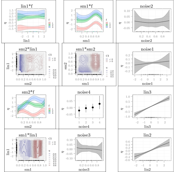
Figure 3: Posterior means and pointwise 80% credible intervals for m1. Interaction surfaces of two numerical covariates are displayed as color coded contour plots, with regions in which the credible interval does not overlap zero marked in blue ($\eta<0$) or red ($\eta>0$). Each panel contains a marginal rug plot that shows where the observations are located. Note that the default behavior of plot.spikeSlabGAM is to cumulate all terms associated with a covariate or covariate combination. In this example, the joint effects of the first 4 covariates sm1, sm2, f and lin1 and the sums of the lin- and sm-terms associated with lin2, lin3, noise1, noise2 and noise3 are displayed. All effects of the noise variables are $\approx 0$, note the different scales on the vertical axes. Vertical axes can be forced to the same range by setting option commonEtaScale.

Figure 3 shows the estimated effects for m1.

Plots for specific terms can be requested with the label argument, Figures 4 and 5 show code snippets and their output for $f(\mathtt{sm1})$ and $f(\mathtt{sm2,f})$. The fits are quite close to the truth despite the heavy-tailed errors and the many noise terms included in the model. Full disclosure: The code used to render Figures 4 and 5 is a little more intricate than the code snippets we show, but the additional code only affects details (font and margin sizes and the arrangement of the panels).

R> plot(m, labels = c("lin(sm1)", "sm(sm1)"), cumulative = FALSE) R> trueFsm1 <- data.frame(truth = fsm1 - mean(fsm1), sm1 = sm1) R> plot(m, labels = "sm(sm1)", ggElems = list(geom_line(aes(x = sm1, + y = truth), data = trueFsm1, linetype = 2)))

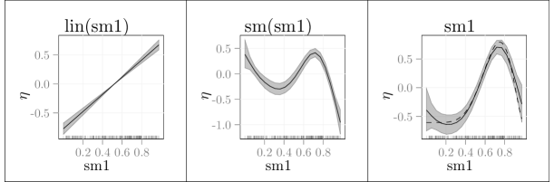
Figure 4: Posterior means and pointwise 80% credible intervals for $f(\mathtt{sm1})$ in m1. Left and middle panel show the separate lin()- and sm()-terms returned by the first call to plot, right panel shows their sum. True shape of $f(\mathtt{sm1})$ added as a dashed line with the ggElems option of plot.spikeSlabGAM.

R> trueFsm2f <- data.frame(truth = fsm2f - mean(fsm2f), + sm2 = sm2, f = f) R> plot(m, labels = "sm(sm2):fct(f)", ggElems = list(geom_line(aes(x = sm2, + y = truth, colour = f), data = trueFsm2f, linetype = 2)))

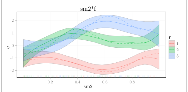
Figure 5: Posterior means and pointwise 80% credible intervals for $f(\mathtt{sm2},\mathtt{f})$ in m1. True shape of $f(\mathtt{sm2}|\mathtt{f})$ added as dashed line for each level of f.

4.3 Assessing convergence

spikeSlabGAM uses the convergence diagnostics implemented in R2WinBUGS (Sturtz et al., 2005). The function ssGAM2Bugs() converts the posterior samples for a spikeSlabGAM-object into a bugs-object, for which graphical and numerical convergence diagnostics are available via plot and print. Note that not all cases of non-convergence should be considered problematic, e.g., if one of the chains samples from a different part of the model space than the others, but has converged on that part of the parameter space.

4.4 Pima indian diabetes

We use the time-honored Pima Indian Diabetes dataset as an example for real non-gaussian data: This dataset from the UCI repository (Newman et al., 1998) is provided in package mlbench (Leisch and Dimitriadou, 2010) as PimaIndiansDiabetes2. We remove two columns with a large number of missing values and use the complete measurements of the remaining 7 covariates and the response (diabetes Yes/No) for 524 women to estimate the model. We set aside 200 observations as a test set: R> data("PimaIndiansDiabetes2", package = "mlbench") R> pimaDiab <- na.omit(PimaIndiansDiabetes2[, -c(4, 5)]) R> pimaDiab <- within(pimaDiab, + diabetes <- 1 * (diabetes == "pos") + ) R> set.seed(1109712439) R> testInd <- sample(1:nrow(pimaDiab), 200) R> pimaDiabTrain <- pimaDiab[-testInd, ] Note that spikeSlabGAM() always expects a dataset without any missing values and responses between 0 and 1 for binomial models.

We increase the length of the burn-in phase for each chain from 100 to 500 iterations and run 8 parallel chains for an additive main effects model (if either multicore (Urbanek, 2010) or snow (Tierney et al., 2010) are installed, the chains will be run in parallel): R> mcmc <- list(nChains = 8, chainLength = 1000, burnin = 500, + thin = 5) R> m0 <- spikeSlabGAM(diabetes   pregnant + glucose + pressure + + mass + pedigree + age, family = "binomial", data = pimaDiabTrain, + mcmc = mcmc) We compute the posterior predictive means for the test set, and request a summary of the fitted model: R> pr0 <- predict(m0, newdata = pimaDiab[testInd, ]) R> print(summary(m0), printModels = FALSE) Spike-and-Slab STAR for Binomial data

Model: diabetes   (lin(pregnant) + sm(pregnant)) + (lin(glucose) + sm(glucose)) + (lin(pressure) + sm(pressure)) + (lin(mass) + sm(mass)) + (lin(pedigree) + sm(pedigree)) + (lin(age) + sm(age)) 524 observations; 58 coefficients in 13 model terms.

Prior: a[tau] b[tau] v[0] a[w] b[w] 5.0e+00 2.5e+01 2.5e-04 1.0e+00 1.0e+00

MCMC: Saved 8000 samples from 8 chain(s), each ran 5000 iterations after a burn-in of 500 ; Thinning: 5 P-IWLS acceptance rates: 0.92 for alpha; 0.64 for xi.

Null deviance: 676 Mean posterior deviance: 474

Marginal posterior inclusion probabilities and term importance: P(gamma=1) pi dim u NA NA 1 lin(pregnant) 0.120 0.009 1 sm(pregnant) 0.018 0.000 8 lin(glucose) 1.000 0.517 1 *** sm(glucose) 0.020 0.000 9 lin(pressure) 0.020 -0.001 1 sm(pressure) 0.011 0.000 9 lin(mass) 1.000 0.237 1 *** sm(mass) 0.628 0.035 9 ** lin(pedigree) 0.024 0.001 1 sm(pedigree) 0.370 -0.002 8 * lin(age) 0.511 0.039 1 ** sm(age) 0.896 0.164 8 ** *:P(gamma=1)>.25 **:P(gamma=1)>.5 ***:P(gamma=1)>.9 spikeSlabGAM selects nonlinear effects for age and mass and a linear trend in glucose. The nonlinear effect of pedigree has fairly weak support. mboost::gamboost ranks the variables very similarly, based on the relative selection frequencies of the associated baselearners: R> b <- gamboost(as.factor(diabetes)   pregnant + glucose + + pressure + mass + pedigree + age, family = Binomial(), + data = pimaDiabTrain)[300] R> aic <- AIC(b, method = "classical") R> prB <- predict(b[mstop(aic)], newdata = pimaDiab[testInd, + ]) R> summary(b[mstop(aic)])$selprob\Soutput bbs(mass,df=dfbase)bbs(glucose,df=dfbase)0.2903230.266129bbs(age,df=dfbase)bbs(pedigree,df=dfbase)0.2096770.120968bbs(pregnant,df=dfbase)bbs(pressure,df=dfbase)0.0725810.040323Finally,wecomparethedevianceonthetestsetforthetwofittedmodels:\Schunk\Sinput R>dev<-function(y,p){+-2*sum(dbinom(x=y,size=1,prob=p,log=T))+}R>c(spikeSlabGAM=dev(pimaDiab[testInd,"diabetes"],pr0),+gamboost=dev(pimaDiab[testInd,"diabetes"],plogis(prB)))\Soutput spikeSlabGAMgamboost180.51194.79Soitseemslike\code{spikeSlabGAM}^{\prime}smodelaveragedpredictionsarealittlemoreaccuratethanthepredictionsreturnedby\code{gamboost}inthiscase.\par Wecancheckthesensitivityoftheresultstothehyperparametersandrefitthemodelwithalarger$v_0$toseeif/howtheresultschange:\Schunk\Sinput R>hyper1<-list(gamma=c(v0=0.005))R>m1<-spikeSlabGAM(diabetes~{}pregnant+glucose+pressure++mass+pedigree+age,family="binomial",data=pimaDiabTrain,+mcmc=mcmc,hyperparameters=hyper1)R>pr1<-predict(m1,newdata=pimaDiab[testInd,])\Schunk\Sinput R>print(summary(m1),printModels=FALSE)\Soutput Spike-and-SlabSTARforBinomialdata\par Model:diabetes~{}(lin(pregnant)+sm(pregnant))+(lin(glucose)+sm(glucose))+(lin(pressure)+sm(pressure))+(lin(mass)+sm(mass))+(lin(pedigree)+sm(pedigree))+(lin(age)+sm(age))524observations;58coefficientsin13modelterms.\par Prior:a[tau]b[tau]v[0]a[w]b[w]5.00025.0000.0051.0001.000\par MCMC:Saved8000samplesfrom8chain(s),eachran5000iterationsafteraburn-inof500;Thinning:5P-IWLSacceptancerates:0.85foralpha;0.64forxi.\par Nulldeviance:676Meanposteriordeviance:458\par Marginalposteriorinclusionprobabilitiesandtermimportance:P(gamma=1)pidimuNANA1lin(pregnant)0.0690.0031sm(pregnant)0.080-0.0018lin(glucose)1.0000.4471***sm(glucose)0.0790.0009lin(pressure)0.117-0.0101sm(pressure)0.0670.0009lin(mass)1.0000.2401***sm(mass)0.9730.0679***lin(pedigree)0.1480.0081sm(pedigree)0.2980.0048*lin(age)0.9610.0891***sm(age)0.9960.1538****:P(gamma=1)>.25**:P(gamma=1)>.5***:P(gamma=1)>.9\Sinput R>(dev(pimaDiab[testInd,"diabetes"],pr1))\Soutput[1]177.85Theselectedtermsareverysimilar,andthepredictionisslightlymoreaccurate(predictivedeviancefor\code{m0}was180.51).Notethat,duetothemulti-modalityofthetargetposterior,stableestimationofpreciseposteriorinclusionandmodelprobabilitiesrequiresmoreparallelchainsthanwereusedinthisexample.\par$

5 Summary

We have presented a novel approach for Bayesian variable selection, model choice, and regularized estimation in (geo-)additive mixed models for Gaussian, binomial, and Poisson responses implemented in spikeSlabGAM. The package uses the established R formula syntax so that complex models can be specified very concisely. It features powerful and user friendly visualizations of the fitted models. Major features of the software have been demonstrated on an example with artificial data with t-distributed errors and on the Pima Indians Diabetes data set. In future work, the author plans to add capabilities for "always included" semiparametric terms and for sampling the inclusion indicators under hierarchical constraints, i.e., never including an interaction if the associated main effects are excluded.

References

- Bae and Mallick (2004) Bae K, Mallick B (2004). “Gene Selection Using a Two-Level Hierarchical Bayesian Model.” Bioinformatics, 20(18), 3423–3430.
- Baglama and Reichel (2006) Baglama J, Reichel L (2006). “Augmented Implicitly Restarted Lanczos Bidiagonalization Methods.” SIAM Journal on Scientific Computing, 27(1), 19–42.
- Brezger et al. (2005) Brezger A, Kneib T, Lang S (2005). “\proglangBayesX: Analyzing Bayesian Structural Additive Regression Models.” Journal of Statistical Software, 14(11).
- Carvalho et al. (2010) Carvalho C, Polson N, Scott J (2010). “The Horseshoe Estimator for Sparse Signals.” Biometrika, 97(2), 465–480.
- Cottet et al. (2008) Cottet R, Kohn R, Nott D (2008). “Variable Selection and Model Averaging in Semiparametric Overdispersed Generalized Linear Models.” Journal of the American Statistical Association, 103(482), 661–671.
- Fahrmeir et al. (2010) Fahrmeir L, Kneib T, Konrath S (2010). “Bayesian Regularisation in Structured Additive Regression: a Unifying Perspective on Shrinkage, Smoothing and Predictor Selection.” Statistics and Computing, 20(2), 203–219.
- Fahrmeir et al. (2004) Fahrmeir L, Kneib T, Lang S (2004). “Penalized Structured Additive Regression for Space-Time Data: a Bayesian Perspective.” Statistica Sinica, 14, 731–761.
- Frühwirth-Schnatter and Wagner (2010) Frühwirth-Schnatter S, Wagner H (2010). “Bayesian Variable Selection for Random Intercept Modelling of Gaussian and Non-Gaussian Data.” In J Bernardo, M Bayarri, JO Berger, AP Dawid, D Heckerman, AFM Smith, M West (eds.), Bayesian Statistics 9. Oxford University Press.
- Gelman et al. (2008) Gelman A, Van Dyk D, Huang Z, Boscardin J (2008). “Using Redundant Parameterizations to Fit Hierarchical Models.” Journal of Computational and Graphical Statistics, 17(1), 95–122.
- George and McCulloch (1993) George E, McCulloch R (1993). “Variable Selection via Gibbs Sampling.” Journal of the American Statistical Association, 88(423), 881–889.
- Gu (1992) Gu C (1992). “Diagnostics for Nonparametric Regression Models with Additive Terms.” Journal of the American Statistical Association, 87(420), 1051–1058.
- Han and Carlin (2001) Han C, Carlin B (2001). “Markov Chain Monte Carlo Methods for Computing Bayes Factors.” Journal of the American Statistical Association, 96(455), 1122–1132.
- Hothorn et al. (2010) Hothorn T, Buehlmann P, Kneib T, Schmid M, Hofner B (2010). \pkgmboost: Model-Based Boosting. \proglangR package version 2.0-7.
- Ishwaran and Rao (2005) Ishwaran H, Rao J (2005). “Spike and Slab Variable Selection: Frequentist and Bayesian Strategies.” The Annals of Statistics, 33(2), 730–773.
- Kneib (2006) Kneib T (2006). Mixed Model Based Inference in Structured Additive Regression. Dr. Hut Verlag. URL http://edoc.ub.uni-muenchen.de/archive/00005011/.
- Lang and Brezger (2004) Lang S, Brezger A (2004). “Bayesian P-Splines.” Journal of Computational and Graphical Statistics, 13(1), 183–212.
- Leisch and Dimitriadou (2010) Leisch F, Dimitriadou E (2010). \pkgmlbench: Machine Learning Benchmark Problems. \proglangR package version 2.1-0.
- Lewis (2009) Lewis B (2009). \pkgirlba: Fast Partial SVD by Implicitly-Restarted Lanczos Bidiagonalization. \proglangR package version 0.1.1, URL http://www.rforge.net/irlba/.
- Lin and Zhang (2006) Lin Y, Zhang H (2006). “Component selection and smoothing in multivariate nonparametric regression.” The Annals of Statistics, 34(5), 2272–2297.
- Meng and van Dyk (1997) Meng X, van Dyk D (1997). “The EM Algorithm–an Old Folk-Song Sung to a Fast New Tune.” Journal of the Royal Statistical Society B, 59(3), 511–567.
- Mitchell and Beauchamp (1988) Mitchell T, Beauchamp J (1988). “Bayesian Variable Selection in Linear Regression.” Journal of the American Statistical Association, 83(404), 1023–1032.
- Newman et al. (1998) Newman D, Hettich S, Blake C, Merz C (1998). “UCI Repository of machine learning databases.” URL http://www.ics.uci.edu/~mlearn/MLRepository.html.
- Polson and Scott (2010) Polson N, Scott J (2010). “Shrink Globally, Act Locally: Sparse Bayesian Regularization and Prediction.” In J Bernardo, M Bayarri, JO Berger, AP Dawid, D Heckerman, AFM Smith, M West (eds.), Bayesian Statistics 9. Oxford University Press.
- \proglangR Development Core Team (2010) \proglangR Development Core Team (2010). \proglangR: A Language and Environment for Statistical Computing. \proglangR Foundation for Statistical Computing, Vienna, Austria. URL http://www.R-project.org.
- Reich et al. (2009) Reich B, Storlie C, Bondell H (2009). “Variable Selection in Bayesian Smoothing Spline ANOVA Models: Application to Deterministic Computer Codes.” Technometrics, 51(2), 110.
- Rue and Held (2005) Rue H, Held L (2005). Gaussian Markov Random Fields: Theory and Applications. Chapman & Hall.
- Scheipl (2010) Scheipl F (2010). “Normal-Mixture-of-Inverse-Gamma Priors for Bayesian Regularization and Model Selection in Generalized Additive Models.” Technical Report 84, Department of Statistics, LMU M nchen. URL http://epub.ub.uni-muenchen.de/11785/.
- Scheipl (2011) Scheipl F (2011). Bayesian Regularization and Model Choice in Structured Additive Regression. Dr. Hut Verlag. URL http://edoc.ub.uni-muenchen.de/13005/.
- Sturtz et al. (2005) Sturtz S, Ligges U, Gelman A (2005). “\pkgR2WinBUGS: A Package for Running WinBUGS from R.” Journal of Statistical Software, 12(3), 1–16.
- Tierney et al. (2010) Tierney L, Rossini A, Li N, Sevcikova H (2010). \pkgsnow: Simple Network Of Workstations. \proglangR package version 0.3-3.
- Urbanek (2010) Urbanek S (2010). \pkgmulticore: Parallel Processing of R Code on Machines with Multiple Cores or CPUs. \proglangR package version 0.1-3, URL http://www.rforge.net/multicore/.
- Wahba et al. (1995) Wahba G, Wang Y, Gu C, Klein R, Klein B (1995). “Smoothing Spline ANOVA for Exponential Families, with Application to the Wisconsin Epidemiological Study of Diabetic Retinopathy.” The Annals of Statistics, 23(6), 1865–1895.
- Wickham (2009) Wickham H (2009). \pkgggplot2: Elegant Graphics for Data Analysis. Springer-Verlag. URL http://had.co.nz/ggplot2/book.
- Wood (2006) Wood S (2006). Generalized Additive Models: an Introduction with R. CRC Press.
- Wood et al. (2002) Wood S, Kohn R, Shively T, Jiang W (2002). “Model Selection in Spline Nonparametric Regression.” Journal of the Royal Statistical Society B, 64(1), 119–139.
- Yau et al. (2003) Yau P, Kohn R, Wood S (2003). “Bayesian Variable Selection and Model Averaging in High-Dimensional Multinomial Nonparametric Regression.” Journal of Computational and Graphical Statistics, 12(1), 23–54.