Relaxing Tight Frame Condition in Parallel Proximal Methods for Signal Restoration

Abstract

A fruitful approach for solving signal deconvolution problems consists of resorting to a frame-based convex variational formulation. In this context, parallel proximal algorithms and related alternating direction methods of multipliers have become popular optimization techniques to approximate iteratively the desired solution. Until now, in most of these methods, either Lipschitz differentiability properties or tight frame representations were assumed. In this paper, it is shown that it is possible to relax these assumptions by considering a class of non necessarily tight frame representations, thus offering the possibility of addressing a broader class of signal restoration problems. In particular, it is possible to use non necessarily maximally decimated filter banks with perfect reconstruction, which are common tools in digital signal processing. The proposed approach allows us to solve both frame analysis and frame synthesis problems for various noise distributions. In our simulations, it is applied to the deconvolution of data corrupted with Poisson noise or Laplacian noise by using (non-tight) discrete dual-tree wavelet representations and filter bank structures.

1 Introduction

Many works in signal/image processing are concerned with data restoration problems. For such problems, the original data $\overline{y}\in\boldsymbol{\ell}^{2}(\mathbb{Z})$ is degraded by a stable convolutive operator $T\colon\boldsymbol{\ell}^{2}(\mathbb{Z})\to\boldsymbol{\ell}^{2}(\mathbb{Z})$ and by a non-necessarily additive noise. The resulting observation model can be written as $z=\mathcal{D}_{\alpha}(T\overline{y})$ where $\mathcal{D}_{\alpha}$ denotes the noise effect and $\alpha>0$ is some related parameter (for example, $\alpha$ may represent the variance for Gaussian noise or the scaling parameter for Poisson noise). In this context, our objective is to recover a signal $y\in\boldsymbol{\ell}^{2}(\mathbb{Z})$, the closest possible to $\overline{y}$, from the observation vector $z$ assumed to belong to $\boldsymbol{\ell}^{2}(\mathbb{Z})$ and available prior information (sparsity, positivity,…). In early works, this problem was solved, mainly for Gaussian noise, by using Wiener filtering, or equivalently quadratic regularization techniques. Later, multiresolution analyses were used for denoising by applying a thresholding to the generated coefficients [2]. Then, in order to improve the denoising performance, redundant frame representations were substituted for wavelet bases [3, 4]. In [5, 6, 7, 8], authors considered convex optimization techniques to jointly address the effects of a noise and of a linear degradation within a convex variational framework. When the noise is Gaussian, the forward-backward (FB) algorithm [5] (also known as thresholded Landweber algorithm when the regularization term is an $\boldsymbol{\ell}_{1}$-norm [6, 7, 8]) and its extensions [9, 10] can be employed in the context of wavelet basis decompositions and its use can be extended to arbitrary frame representations [11]. However, in the context of a non-additive noise such as a Poisson noise or a Laplace noise, FB algorithm is no longer applicable due to the non-Lipschitz differentiability of the data fidelity term. Other convex optimization algorithms must be employed such as the Douglas-Rachford (DR) algorithm [12], the Parallel ProXimal Algorithm (PPXA) [13] or the Alternating Direction Method of Multipliers (ADMM) [14, 15]. These algorithms belong to the class of proximal algorithms and, for tractability issues, they often require to use tight frame representation for which closed forms of the involved proximity operators can be derived [13, 14, 15, 16]. The goal of this paper is to propose a way to relax the tight frame requirement by considering an appropriate class of frame representations.

In the following, we consider two general convex minimization problems, which are useful to solve frame-based restoration problems formulated under a Synthesis Form (SF) or an Analysis Form (AF). The SF can be expressed as:

$$\underset{\begin{subarray}{c}y=F^{*}x,\;x\in\boldsymbol{\ell}^{2}(\mathbb{Z})\end{subarray}}{\operatorname{minimize}}\;\sum_{r=1}^{R}f_{r}(L_{r}y)+\sum_{s=1}^{S}g_{s}(x)$$ (1)

and the AF is:

$$\underset{y\in\boldsymbol{\ell}^{2}(\mathbb{Z})}{\operatorname{minimize}}\;\sum_{r=1}^{R}f_{r}(L_{r}y)+\sum_{s=1}^{S}g_{s}(Fy).$$ (2)

$F\colon\boldsymbol{\ell}^{2}(\mathbb{Z})\to\boldsymbol{\ell}^{2}(\mathbb{Z})$ (resp. $F^{*}\colon\boldsymbol{\ell}^{2}(\mathbb{Z})\to\boldsymbol{\ell}^{2}(\mathbb{Z})$) denotes the frame analysis (resp. synthesis) operator. For every $r\in\{1,\ldots,R\}$, $f_{r}\colon\boldsymbol{\ell}^{2}(\mathbb{Z})\to\left]-\infty,+\infty\right]$ is a convex, lower semicontinuous, and proper function, $L_{r}\colon\boldsymbol{\ell}^{2}(\mathbb{Z})\to\boldsymbol{\ell}^{2}(\mathbb{Z})$ is a stable convolutive operator, and for every $s\in\{1,\ldots,S\}$, $g_{s}\colon\boldsymbol{\ell}^{2}(\mathbb{Z})\to\left]-\infty,+\infty\right]$ is a convex, lower semicontinuous, and proper function. In several works, SF has been preferred since AF appears to be more difficult to solve numerically [17, 18, 19, 20]. In the proposed framework, both approaches have a similar complexity.

This paper is organized as follows: in Section 2, the class of frames considered in this work is defined and their connections with filter bank structures is emphasized. In Section 3, we show how these (non necessarily tight) frames can be combined with parallel proximal algorithms in order to solve Problems (1) and (2). The proposed approach is also applicable to related augmented Lagrangian approaches. Finally, restoration results are provided in Section 4 for scenarios involving Poisson noise or Laplace noise by using Dual-Tree Transforms (DTT) and filter bank representations.

Notation: Throughout this paper, $\Gamma_{0}(\mathcal{H})$ designates the class of lower semicontinuous convex functions $\varphi$ defined on a real Hilbert space $\mathcal{H}$ and taking their values in $\left]-\infty,+\infty\right]$, which are proper in the sense that their domain $\operatorname{dom}\varphi=\big{\{}{u\in\mathcal{H}}~{}\big{|}~{}{\varphi(u)<{+\infty}}\big{\}}$ is nonempty. If $\varphi\in\Gamma_{0}(\mathcal{H})$ has a unique minimizer, it is denoted by $\underset{u\in\mathcal{H}}{\operatorname{argmin}}\varphi(u)$. The interior of a set $C$ is denoted by $\operatorname{int}C$.

2 Frame representations

2.1 Definitions

Physical properties of the target signal $\overline{y}\in\boldsymbol{\ell}^{2}(\mathbb{Z})$, such as sparsity or spatial regularity, may be suitably expressed in terms of its coefficients $\overline{x}=(\overline{x}(k))_{k\in\mathbb{Z}}\in\boldsymbol{\ell}^{2}(\mathbb{Z})$ where $\overline{y}=\sum_{k=-\infty}^{+\infty}\overline{x}(k)e_{k}$ and $(e_{k})_{k\in\mathbb{Z}}$ denotes a dictionary of signals in $\boldsymbol{\ell}^{2}(\mathbb{Z})$. Such a dictionary constitutes a frame if there exist two constants $\underline{\mu}$ and $\overline{\mu}$ in $\left]0,+\infty\right[$ such that

$$\big{(}\forall y\in\boldsymbol{\ell}^{2}(\mathbb{Z})\big{)}\qquad\underline{\mu}\|y\|^{2}\leq\sum_{k=-\infty}^{+\infty}|{\left\langle{{y}\mid{e_{k}}}\right\rangle}|^{2}\leq\overline{\mu}\|y\|^{2}.$$ (3)

The associated frame operator is the injective linear operator defined as

$$\big{(}\forall y\in\boldsymbol{\ell}^{2}(\mathbb{Z})\big{)}\qquad Fy=\big{(}{\left\langle{{y}\mid{e_{k}}}\right\rangle}\big{)}_{k\in\mathbb{Z}},$$ (4)

the adjoint of which is the surjective linear operator given by

$$\big{(}\forall x=\big{(}x(k)\big{)}_{k\in\mathbb{Z}}\in\boldsymbol{\ell}^{2}(\mathbb{Z})\big{)}\qquad F^{*}x=\sum_{k=-\infty}^{+\infty}x(k)\,e_{k}.$$ (5)

When $F^{-1}=F^{*}$, an orthonormal basis is obtained. Further constructions as well as a detailed account of frame theory in Hilbert spaces can be found in [21].

A tight frame is such that, for some $\mu\in\left]0,+\infty\right[$, $F^{*}F=\mu\operatorname{I}\,$ where $\operatorname{I}\,$ denotes the identity operator. In Condition (3), this means that $\underline{\mu}=\overline{\mu}=\mu$. A simple example of a tight frame is the union of $\mu$ orthonormal bases. Other examples of tight frames can be found in [22, 23, 24].

2.2 A class of non necessarily tight frames

We consider a linear operator $F$ which is basically obtained by cascading a non necessarily maximally decimated filter bank and a semi-orthogonal transform. A linear operator $U\colon\big{(}\boldsymbol{\ell}^{2}(\mathbb{Z})\big{)}^{N}\rightarrow\big{(}\boldsymbol{\ell}^{2}(\mathbb{Z})\big{)}^{Q}$, with $N\in\mathbb{N}^{*}$ and $Q\in\mathbb{N}^{*}$, is said to be semi-orthogonal if there exists $\mu_{U}\in\left]0,+\infty\right[$ such that $U^{*}U=\mu_{U}\operatorname{I}\,$. Recall that an analysis filter bank can be put under its polyphase form by performing a polyphase decomposition $\Pi_{D}$ followed by a real MIMO (Multi-Input Multi-Output) filtering $V$ [25]:
•  the polyphase decomposition $\Pi_{D}$ is an operator from $\boldsymbol{\ell}^{2}(\mathbb{Z})$ to $(\boldsymbol{\ell}^{2}(\mathbb{Z})\big{)}^{D}$ with $D\in\mathbb{N}^{*}$ such that, for every $y=\big{(}y(n)\big{)}_{n\in\mathbb{Z}}\in\boldsymbol{\ell}^{2}(\mathbb{Z})$, $\Pi_{D}y=(y^{(j)})_{1\leq j\leq D}$ where $y^{(j)}=\big{(}y(Dn-j+1)\big{)}_{n\in\mathbb{Z}}$ is the $j$-th polyphase component of order $D$ of the signal $y$. The adjoint operator of $\Pi_{D}$ is given by $\Pi_{D}^{*}\colon(\boldsymbol{\ell}^{2}(\mathbb{Z})\big{)}^{D}\to\boldsymbol{\ell}^{2}(\mathbb{Z})\colon(y^{(j)})_{1\leq j\leq D}\mapsto u=\big{(}u(n)\big{)}_{n\in\mathbb{Z}}$ where, for every $n\in\mathbb{Z}$ and $j\in\{1,\ldots,D\}$, $u(Dn-j+1)=y^{(j)}(n)$. So, $\Pi_{D}^{*}$ allows us to concatenate $D$ square summable sequences into a single one. It can be noticed that $\Pi_{D}^{*}\Pi_{D}=\operatorname{I}\,$ and $\Pi_{D}\Pi_{D}^{*}=\operatorname{I}\,$, which means that $\Pi_{D}$ is an isometry and $\Pi_{D}^{-1}=\Pi_{D}^{*}$.
•  The MIMO filter $V$ is defined as

$$V=\begin{bmatrix}V_{1,1}&\ldots&V_{1,D}\\ \vdots&&\vdots\\ V_{N,1}&\ldots&V_{N,D}\\ \end{bmatrix}$$ (6)

where, for every $i\in\{1,\ldots,N\}$ and $j\in\{1,\ldots,D\}$, $V_{i,j}\colon\boldsymbol{\ell}^{2}(\mathbb{Z})\to\boldsymbol{\ell}^{2}(\mathbb{Z})$ is a SISO (Single-Input Single-Output) stable filter. Hence, the impulse response of this filter belongs to $\boldsymbol{\ell}^{1}(\mathbb{Z})$ and its frequency response $\widehat{v}_{i,j}$ is a continuous function. In addition, it is assumed that $V$ is left invertible, that is: for every $\nu\in[-1/2,1/2]$, the rank of the matrix $\widehat{\boldsymbol{v}}(\nu)=[\widehat{v}_{i,j}(\nu)]_{1\leq i\leq N,1\leq j\leq D}$ is equal to $D$. The adjoint operator of $V$ is the $D\times N$ MIMO filter given by

$$V^{*}=\begin{bmatrix}V_{1,1}^{*}&\ldots&V_{N,1}^{*}\\ \vdots&&\vdots\\ V_{1,D}^{*}&\ldots&V_{N,D}^{*}\\ \end{bmatrix}$$ (7)

where, for every $i\in\{1,\ldots,N\}$ and $j\in\{1,\ldots,D\}$, $V_{i,j}^{*}$ is the SISO filter with complex conjugate frequency response $\widehat{v}_{i,j}^{*}$.
We have then the following result (the proof is provided in Appendix 5.1):

Proposition 2.1

The operator $F=\Pi_{Q}^{*}UV\Pi_{D}$ is a frame operator with frame constants $\underline{\mu}=$$\inf_{\nu\in[-1/2,1/2]}\sigma_{\rm min}(\nu)$ and $\overline{\mu}=\sup_{\nu\in[-1/2,1/2]}\sigma_{\rm max}(\nu)$, where, for every $\nu$, $\sigma_{\rm min}(\nu)\in\left]0,+\infty\right[$ and $\sigma_{\rm max}(\nu)\in\left]0,+\infty\right[$ are the minimum and maximum eigenvalues of $\widehat{\boldsymbol{v}}(\nu)^{\rm H}\widehat{\boldsymbol{v}}(\nu)$. In addition, we have:

$$F^{*}F=\mu_{U}\Pi_{D}^{*}V^{*}V\Pi_{D}.$$ (8)

The resulting frame is not necessarily tight. However, when $(\forall\nu\in[-1/2,1/2])$ $\widehat{v}(\nu)^{\rm H}\widehat{v}(\nu)=\operatorname{I}_{D}\,$, the frame is tight. This includes paraunitary systems $V$ as particular cases when $D=N$.

Below, we provide examples of popular transforms in signal processing which belong to the class of considered frame representations.

2.2.1 Example 1 – Dual-tree transforms

In order to obtain low redundancy representations, frames such as the 2D $M$-band DTT have been proposed [26, 27, 28]. The real (resp. complex) DTT consists of performing $N=2$ (resp. $N=4$) $M$-band orthonormal wavelet decompositions in parallel where, for every $i\in\{1,\ldots,N\}$, $U_{i}\colon\boldsymbol{\ell}^{2}(\mathbb{Z})\rightarrow\boldsymbol{\ell}^{2}(\mathbb{Z})$ denotes the $i$-th orthogonal wavelet transform. An orthogonal combination of the subbands modeled by $\Phi\colon\big{(}\boldsymbol{\ell}^{2}(\mathbb{Z})\big{)}^{N}\rightarrow\big{(}\boldsymbol{\ell}^{2}(\mathbb{Z})\big{)}^{N}$ is applied to ensure directionality properties. $(U_{i})_{1\leq i\leq N}$ and $\Phi$ are related to $U$ by the following relation:

$$U=\Phi\;\begin{bmatrix}U_{1}&0&\ldots&0\\ 0&U_{2}&\ddots&\vdots\\ \vdots&\ddots&\ddots&0\\ 0&\ldots&0&U_{N}\\ \end{bmatrix}.$$ (9)

Since $\Phi^{*}\Phi=\Phi\Phi^{*}=\operatorname{I}\,$ and, for every $i\in\{1,\ldots,N\}$, $U_{i}^{*}U_{i}=U_{i}U_{i}^{*}=\operatorname{I}\,$, $U$ is an orthogonal transform. In the general form of DTT, each orthonormal wavelet decomposition is preceded by a prefiltering stage related to the discretization process. More precisely, it takes the form:

$$V=\begin{bmatrix}V_{1,1}^{*}\;\ldots\;V_{N,1}^{*}\end{bmatrix}^{*}.$$ (10)

The variables $Q$ and $D$ as defined before are thus equal to $N$ and $1$, respectively. The left invertibility condition here reduces to the fact that the frequency response $|\widehat{v}_{1,1}|^{2}+\cdots+|\widehat{v}_{N,1}|^{2}$ does not vanish. Note that, due to the presence of prefilters, the discrete DTT is not a tight frame in general. Furthermore, an extended class of DTTs can be obtained by using tight frame overcomplete representations $(U_{i})_{1\leq i\leq N}$ having the same frame constant $\mu_{U}$ (e.g. redundant wavelet representations derived from orthogonal filters after appropriate renormalization), in which case $U$ as defined by (9) is a semi-orthogonal transform.

2.2.2 Example 2 – Filter banks

Analysis filter banks with perfect reconstruction correspond to the case when $U=\operatorname{I}\,$ and $Q=N$. $D$ is the decimation factor and $N$ is the number of channels. The redundancy introduced by such a filter bank structure is $N/D\geq 1$. More details about filter bank design can be found in [29]. Lapped transforms [30] can also be implemented with filter bank structures. As already mentioned, filter banks do not constitute tight frames in general. Note that if $D=1$, a fully undecimated filter bank is obtained.

Tight frame representations have been widely used for data recovery by using convex optimization methods. In the next section, we recall some convex optimization tools and show the relevance of the considered class of frames in recent optimization approaches.

3 Use of parallel proximal algorithms

A number of algorithms such as the alternating split Bregman algorithm [31], augmented Lagrangian techniques [14] and parallel proximal methods [32] have been recently proposed to address possibly nonsmooth convex optimization problems encountered in the solution of restoration problems. Here, we will focus on this specific class of algorithms which have proven to be useful for solving problems like (1) and (2) when a tight frame representation is employed. A common feature of the aforementioned algorithms is that they require a large-size linear system to be solved at each iteration. When non tight frame representations are used, the computational cost of the associated inversion may become prohibitive. We will see however that for the class of frames introduced in Section 2, this inversion can be performed in an efficient manner. This fact will be demonstrated by considering an extension of the Parallel ProXimal Algorithm (PPXA), hereafter designated as PPXA+. As shown in [32], PPXA+ is closely related to the alternating direction method of multipliers and its parallel extensions [15].

We recall that the proximity operator [33] of a function $\varphi\in\Gamma_{0}(\mathcal{H})$ is defined as

$$\operatorname{prox}_{\varphi}\colon\mathcal{H}\to\mathcal{H}\colon v\mapsto\arg\min_{u\in\mathcal{H}}\displaystyle{\frac{1}{2}}\left\|u-v\right\|^{2}+\varphi(u).$$ (11)

It can be observed that when $\varphi$ is the indicator function $\iota_{C}$ of a nonempty closed convex subset $C$ of $\mathcal{H}$, i.e. it takes on the value $0$ in $C$ and ${+\infty}$ in $\mathcal{H}\setminus C$, $\operatorname{prox}_{\iota_{C}}$ reduces to the projector $P_{C}$ onto $C$. Other examples of proximity operators corresponding to potential functions of standard log-concave univariate probability densities have been listed in [5, 11, 13]. The proximity operators employed in the experimental part of this paper, are recalled below.

Example 3.1

(soft-thresholding rule)
Let $\alpha>0$, and set $\varphi\colon\mathbb{R}\to\mathbb{R}\colon\xi\mapsto\alpha|\xi|$. Then, for every $\xi\in\mathbb{R}$, $\operatorname{prox}_{\varphi}\xi=\operatorname{sign}(\xi)\max\{|\xi|-\alpha,0\}$.

Example 3.2

(Poisson minus log-likelihood function) [11]
Let $\alpha>0$, $\chi\geq 0$, and set

$$\varphi\colon \mathbb{R}\to\left]-\infty,+\infty\right]\colon\xi\mapsto\begin{cases}-\chi\ln(\xi)+\alpha\xi,&\text{if}\;\;\chi>0\;\text{and}\;\xi>0;\\ \alpha\xi,&\text{if}\;\;\chi=0\;\text{and}\;\xi\geq 0;\\ {+\infty},&\text{otherwise}.\end{cases}$$ (12)

Then, for every $\xi\in\mathbb{R}$,

$$\operatorname{prox}_{\varphi}\xi=\frac{\xi-\alpha+\sqrt{|\xi-\alpha|^{2}+4\chi}}{2}.$$ (13)

One of the difficulties in the resolution of problems like (1) or (2) is that they involve linear operators. Unfortunately, the proximity operator of the composition of a linear operator and a convex function takes a closed form expression only under restrictive assumptions as stated below:

Proposition 3.3

[12]
Let $\mathcal{G}$ be a real Hilbert space, $\varphi\in\Gamma_{0}(\mathcal{G})$ and let $L\colon\mathcal{H}\rightarrow\mathcal{G}$ denote a bounded linear operator. Suppose that $LL^{*}=\chi\operatorname{I}\,$, for some $\chi\in\left]0,+\infty\right[$. Then, $\varphi\circ L\in\Gamma_{0}(\mathcal{H})$ and $\operatorname{prox}_{\varphi\circ L}=\operatorname{I}\,+\chi^{-1}L^{*}(\operatorname{prox}_{\chi\varphi}-\operatorname{I}\,)L$.

When dealing with linear operators $L$ such that $LL^{*}\neq\chi\operatorname{I}\,$ for any $\chi>0$, proximal algorithms requiring the inversion of a linear operator at each iteration can however be designed. For example, Algorithm 1 (resp. Algorithm 2) can be applied to Problem (1) (resp. Problem (2)). (In these algorithms, the sequences $(a_{r,\ell})_{1\leq r\leq R}$ and $(b_{s,\ell})_{1\leq s\leq S}$ model possible numerical errors in the computation of the proximity operators at iteration $\ell$.)

Algorithm 1

  Initialization $\left\lfloor\begin{array}[]{l}(\eta_{r})_{1\leq r\leq R}\in\left]0,+\infty\right[^{R},(\kappa_{s})_{1\leq s\leq S}\in\left]0,+\infty\right[^{S};\;(v_{r,0})_{1\leq r\leq R}\in\big{(}\boldsymbol{\ell}^{2}(\mathbb{Z})\big{)}^{R},(w_{s,0})_{1\leq s\leq S}\in\big{(}\boldsymbol{\ell}^{2}(\mathbb{Z})\big{)}^{S}\\ x_{0}=\arg\min_{u\in\boldsymbol{\ell}^{2}(\mathbb{Z})}\sum_{r=1}^{R}\eta_{r}{\|L_{r}F^{*}u-v_{r,0}\|}^{2}+\sum_{s=1}^{S}\kappa_{s}{\|u-w_{s,0}\|}^{2}\\ \end{array}\right.$

  For $\ell=0,1,\ldots$ $\left\lfloor\begin{array}[]{l}\mbox{For}\;\;r=1,\ldots,R\qquad\qquad p_{r,\ell}=\operatorname{prox}_{f_{r}/\eta_{r}}v_{r,\ell}+a_{r,\ell}\\ \mbox{For}\;\;s=1,\ldots,S\qquad\qquad r_{s,\ell}=\operatorname{prox}_{g_{s}/\kappa_{s}}w_{s,\ell}+b_{s,\ell}\\ \lambda_{\ell}\in]0,2[\\ c_{\ell}=\arg\min_{u\in\boldsymbol{\ell}^{2}(\mathbb{Z})}\sum_{r=1}^{R}\eta_{r}{\|L_{r}F^{*}u-p_{r,\ell}\|}^{2}+\sum_{s=1}^{S}\kappa_{s}{\|u-r_{s,\ell}\|}^{2}\\ \mbox{For}\;\;r=1,\ldots,R\qquad\qquad v_{r,\ell+1}=v_{r,\ell}+\lambda_{\ell}\big{(}L_{r}F^{*}(2c_{\ell}-x_{\ell})-p_{r,\ell}\big{)}\\ \mbox{For}\;\;s=1,\ldots,S\qquad\qquad w_{s,\ell+1}=w_{s,\ell}+\lambda_{\ell}\big{(}2c_{\ell}-x_{\ell}-r_{s,\ell}\big{)}\\ x_{\ell+1}=x_{\ell}+\lambda_{\ell}(c_{\ell}-x_{\ell})\\ \end{array}\right.$

Algorithm 2

  Initialization $\left\lfloor\begin{array}[]{l}(\eta_{r})_{1\leq r\leq R}\in\left]0,+\infty\right[^{R},(\kappa_{s})_{1\leq s\leq S}\in\left]0,+\infty\right[^{S};\;(v_{r,0})_{1\leq r\leq R}\in\big{(}\boldsymbol{\ell}^{2}(\mathbb{Z})\big{)}^{R},(w_{s,0})_{1\leq s\leq S}\in\big{(}\boldsymbol{\ell}^{2}(\mathbb{Z})\big{)}^{S}\\ y_{0}=\arg\min_{u\in\boldsymbol{\ell}^{2}(\mathbb{Z})}\sum_{r=1}^{R}\eta_{r}{\|L_{r}u-v_{r,0}\|}^{2}+\sum_{s=1}^{S}\kappa_{s}{\|Fu-w_{s,0}\|}^{2}\\ \end{array}\right.$

  For $\ell=0,1,\ldots$ $\left\lfloor\begin{array}[]{l}\mbox{For}\;\;r=1,\ldots,R\qquad\qquad p_{r,\ell}=\operatorname{prox}_{f_{r}/\eta_{r}}v_{r,\ell}+a_{r,\ell}\\ \mbox{For}\;\;s=1,\ldots,S\qquad\qquad r_{s,\ell}=\operatorname{prox}_{g_{s}/\kappa_{s}}w_{s,\ell}+b_{s,\ell}\\ \lambda_{\ell}\in]0,2[\\ c_{\ell}=\arg\min_{u\in\boldsymbol{\ell}^{2}(\mathbb{Z})}\sum_{r=1}^{R}\eta_{r}{\|L_{r}u-p_{r,\ell}\|}^{2}+\sum_{s=1}^{S}\kappa_{s}{\|Fu-r_{s,\ell}\|}^{2}\\ \mbox{For}\;\;r=1,\ldots,R\qquad\qquad v_{r,\ell+1}=v_{r,\ell}+\lambda_{\ell}\big{(}L_{r}(2c_{\ell}-y_{\ell})-p_{r,\ell}\big{)}\\ \mbox{For}\;\;s=1,\ldots,S\qquad\qquad w_{s,\ell+1}=w_{s,\ell}+\lambda_{\ell}\big{(}F(2c_{\ell}-y_{\ell})-r_{s,\ell}\big{)}\\ y_{\ell+1}=y_{\ell}+\lambda_{\ell}(c_{\ell}-y_{\ell})\\ \end{array}\right.$

The convergence of the sequence $(x_{\ell})_{\ell\in\mathbb{Z}}$ (resp. $(y_{\ell})_{\ell\in\mathbb{Z}}$) generated by Algorithm 1 (resp. Algorithm 2) to an optimal solution of the related optimization problem is guaranteed under the following technical assumptions (see [32] for more details):

Assumption 3.4

2. $\Big{(}\bigcap_{r=1}^{R}\operatorname{int}\operatorname{dom}f_{r}\circ L_{r}F^{*}\big{)}\cap\Big{(}\bigcap_{s=1}^{S-1}\operatorname{int}\operatorname{dom}g_{s}\Big{)}\cap\operatorname{dom}g_{S}\neq{\varnothing}$

3. (resp. $\Big{(}\bigcap_{r=1}^{R}\operatorname{int}\operatorname{dom}f_{r}\circ L_{r}\Big{)}\cap\Big{(}\bigcap_{s=1}^{S-1}\operatorname{int}\operatorname{dom}g_{s}\circ F\Big{)}\cap\operatorname{dom}g_{S}\circ F\neq{\varnothing}$).

4. There exists $\underline{\lambda}\in]0,2[$ such that $(\forall\ell\in\mathbb{N})\;\underline{\lambda}\leq\lambda_{\ell+1}\leq\lambda_{\ell}$.

5. $(\forall r\in\{1,\ldots,R\})$ $\sum_{\ell=0}^{+\infty}\|a_{r,\ell}\|<+\infty$ and $(\forall s\in\{1,\ldots,S\})$ $\sum_{\ell=0}^{{+\infty}}\|b_{s,\ell}\|<+\infty$.

Note that quadratic minimizations need to be performed in the initialization step and in the computation of the intermediate variable $c_{\ell}$ at iteration $\ell$. These amount to inverting a large-size linear operator which is untractable for arbitrary frames. We will now show that the class of frame operators $F$ introduced in Section 2.2 allows us to overcome this difficulty.

To do so, recall that the convolutive operators $(L_{r})_{1\leq r\leq R}$ can be put under a polyphase form [25]:

$$(\forall r\in\{1,\ldots,R\})\qquad L_{r}=W_{r}\Pi_{D}$$ (14)

where the polyphase decomposition operator $\Pi_{D}$ has been defined in Section 2.2 and $W_{r}=[W_{r,1},\ldots,W_{r,D}]$ is a MISO (Multi-Input Single-Output) filter (for every $j\in\{1,\ldots,D\}$, $W_{r,j}\colon\boldsymbol{\ell}^{2}(\mathbb{Z})\to\boldsymbol{\ell}^{2}(\mathbb{Z})$ is a SISO filter). Now, invoking Proposition 2.1 and making use of Sherman-Morrison-Woodbury identity yield:
•   for SF (Algorithm 1)

$$\kappa\Big{(}\sum_{r=1}^{R}\eta_{r}FL_{r}^{*}L_{r}F^{*}+\kappa\operatorname{I}\,\Big{)}^{-1}= \operatorname{I}\,-F\big{(}\sum_{r=1}^{R}\eta_{r}L_{r}^{*}L_{r}\big{)}\Big{(}\kappa\operatorname{I}\,+F^{*}F\big{(}\sum_{r=1}^{R}\eta_{r}L_{r}^{*}L_{r}\big{)}\Big{)}^{-1}F^{*}$$

$$= \operatorname{I}\,-F\Pi_{D}^{*}\big{(}\sum_{r=1}^{R}\eta_{r}W_{r}^{*}W_{r}\big{)}\Pi_{D}\Big{(}\kappa\operatorname{I}\,+\mu_{U}\Pi_{D}^{*}V^{*}V\big{(}\sum_{r=1}^{R}\eta_{r}W_{r}^{*}W_{r}\big{)}\Pi_{D}\Big{)}^{-1}F^{*}$$

$$= \operatorname{I}\,-F\Pi_{D}^{*}\big{(}\sum_{r=1}^{R}\eta_{r}W_{r}^{*}W_{r}\big{)}\Big{(}\kappa\operatorname{I}\,+\mu_{U}V^{*}V\big{(}\sum_{r=1}^{R}\eta_{r}W_{r}^{*}W_{r}\big{)}\Big{)}^{-1}\Pi_{D}F^{*},$$ (15)

•   for AF (Algorithm 2)

$$\Big{(}\sum_{r=1}^{R}\eta_{r}L_{r}^{*}L_{r}+\kappa F^{*}F\Big{)}^{-1} =\Pi_{D}^{*}\Big{(}\sum_{r=1}^{R}\eta_{r}W_{r}^{*}W_{r}+\kappa\mu_{U}V^{*}V\Big{)}^{-1}\Pi_{D},$$ (16)

where $\kappa=\sum_{s=1}^{S}\kappa_{s}$. Note that the idea of using the Woodbury matrix identity to handle the inversion for SF was proposed in [34] in the context of tight frames. The inversions in (3) (resp. (16)) can be performed by noticing that, as $(W_{r})_{1\leq r\leq R}$ and $V$ are multivariate filters with frequency responses $(\widehat{\boldsymbol{w}}_{r})_{1\leq r\leq R}$ and $\widehat{\boldsymbol{v}}$, $\kappa\operatorname{I}\,+\mu_{U}V^{*}V\big{(}\sum_{r=1}^{R}\eta_{r}W_{r}^{*}W_{r}\big{)}$ (resp. $\sum_{r=1}^{R}\eta_{r}W_{r}^{*}W_{r}+\kappa\mu_{U}V^{*}V$) is a MIMO filter with frequency response: for every $\nu\in[-1/2,1/2]$,

$$\kappa\operatorname{I}_{D}\,+\mu_{U}\widehat{\boldsymbol{v}}(\nu)^{\rm H}\widehat{\boldsymbol{v}}(\nu)\big{(}\sum_{r=1}^{R}\eta_{r}\widehat{\boldsymbol{w}}_{r}(\nu)^{\rm H}\widehat{\boldsymbol{w}}_{r}(\nu)\big{)}\qquad\Big{(}\text{resp.}\;\sum_{r=1}^{R}\eta_{r}\widehat{\boldsymbol{w}}_{r}(\nu)^{\rm H}\widehat{\boldsymbol{w}}_{r}(\nu)+\kappa\mu_{U}\widehat{\boldsymbol{v}}(\nu)^{\rm H}\widehat{\boldsymbol{v}}(\nu)\Big{)}.$$ (17)

Hence, by resorting to Fast Fourier Transform implementations, the problem reduces to the inversion of $D\times D$ matrices.

4 Experimental results

We apply the proposed optimization method to the restoration of images degraded by a blur and a Poisson (resp. Laplace) noise. For simplicity sake, the proposed formulation has been presented in the 1D case, but its 2D extension is straightforward. The scaling factor of the Poisson (resp. Laplace) noise is $\alpha=0.1$ (resp. $\alpha=10$). The data fidelity term is related to the Poisson (resp. Laplace) minus log-likelihood, which corresponds to the potential function $\varphi$ defined by (12) (resp. by Example 3.1). In the considered examples, the regularization term simply is an $\boldsymbol{\ell}_{1}$-norm modeling the sparsity of $\overline{y}$ through a frame representation. Two different frames are considered: a (Complex) Dual-Tree Transform, presented in Section 2.2.1, and an eigenfilter bank decomposition [35, 36], which is a special case of the subband structure presented in Section 2.2.2. We constrain the data values to belong to $[0,255]$, so defining a closed convex constraint set $C$. The considered SF (resp. AF) problem is a particular case of Problem (1) (resp. (2)) where $R=2$, $S=1$, $f_{1}=\varphi$, $f_{2}=\iota_{C}$, and $g_{1}=\tau\|\cdot\|_{1}$ with $\tau>0$. The last function corresponds to the regularization term operating in the frame domain. In the considered problems, $L_{1}=T$ and $L_{2}=\operatorname{I}\,$. The proximity operators associated to $f_{1}$, $f_{2}$, and $g_{1}$ are derived from Example 3.2, the projection onto $C$, and Example 3.1. In our simulations, the parameter $\tau$ is empirically chosen to maximize the signal-to-noise-ratio (SNR). In general, the value of this parameter is not the same for FA and FS.

Note that an alternative to the proposed approach consists of resorting to primal-dual algorithms [37, 38, 39, 40, 41]. These algorithms are appealing as they do not require any operator inversion and they can thus be employed with arbitrary frames. However, after appropriate choices for the weights $(\eta_{r})_{1\leq r\leq R}$, $(\kappa_{s})_{1\leq s\leq S}$, and the relaxation parameter $\lambda_{\ell}$, the proposed approach appeared to be faster. For example, similar frequency domain implementations of the Monotone + Skew Forward Backward Forward (M+SFBF) algorithm [41] were observed to be about twenty times slower than the proposed method in term of iterations and computation time.

Figure 1 shows the restoration results for a cropped version of the “Barbara” image in the presence of Poisson noise and a uniform blur of size $5\times 5$. We adopt a SF criterion and we consider a tight version (i.e., for every $i\in\{1,\ldots,4\}$, $V_{i,1}=\operatorname{I}\,$) as well as a non-tight version of Complex DTT. The Complex DTT [28] is computed using symlets of length 6 over 3 resolution levels. In order to efficiently perform the inversions in (3) and (16), fast discrete Fourier diagonalization techniques have been employed. The use of the non-tight Complex DTT including prefilters allows us to improve the quality of the results both visually and in terms of SNR and SSIM [42]. Figure 2 displays a second restoration example for a cropped version of the “Straw” image in the presence of Laplace noise and a uniform blur of size $5\times 5$. AF results are presented by using a DTT and an eigenfilter bank ($D=8$ and $N=14$) computed from the degraded image. This formulation leads to better results than those obtained with SF. Significant gains in favour of the eigenfilter bank can be observed .

​​​​​​
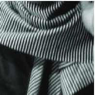
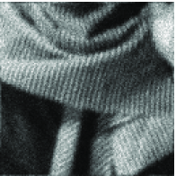
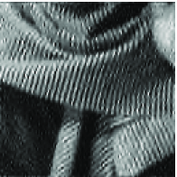
Original	​​​​​​Degraded	Tight-frame Complex DTT	Complex DTT
	SNR = 11.4 dB	SNR = 13.3 dB	SNR = 14.2 dB
	SSIM = 0.53	SSIM = 0.69	SSIM = 0.73

Figure 1: Cropped versions of Barbara image (size $128\times 128$). Restored images using SF and complex DTT.

​​​​​​
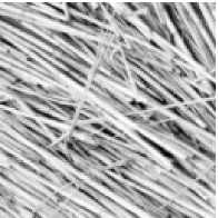
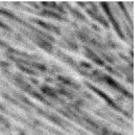
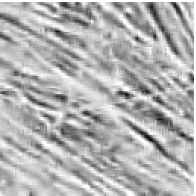
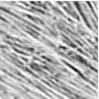
​​​​​​Original	Degraded	DTT	Eigenfilter bank
	SNR = 14.8 dB	SNR = 16.7 dB	SNR = 17.3 dB
	SSIM = 0.42	SSIM = 0.64	SSIM = 0.69

Figure 2: Cropped versions of Straw image (size $128\times 128$). Restored images using AF considering DTT and eigenfilter banks.

5 Appendix

5.1 Proof of Proposition 2.1

Eq. (8) is a direct consequence of the fact that $U$ is semi-orthogonal and $\Pi_{Q}^{*}$ is an isometry. By using Parseval’s formula, for every $y\in\boldsymbol{\ell}^{2}(\mathbb{Z})$,

$$\|Fy\|^{2}=\mu_{U}\|V\Pi_{D}y\|^{2}=\mu_{U}\int_{-1/2}^{1/2}\|\widehat{\boldsymbol{v}}(\nu)\widehat{\boldsymbol{y}}(\nu)\|^{2}d\nu$$ (18)

where $\widehat{\boldsymbol{y}}(\nu)=[\widehat{y}^{(1)}(\nu),\ldots,\widehat{y}^{(D)}(\nu)]^{\top}$, and, for every $j\in\{1,\ldots,D\}$, $\widehat{y}^{(j)}$ is the Fourier transform of the discrete signal $y^{(j)}$. By using the fact that, for every $\nu\in[-1/2,1/2]$, $\sigma_{\rm min}(\nu)\|\widehat{\boldsymbol{y}}(\nu)\|^{2}\leq\|\widehat{\boldsymbol{v}}(\nu)\widehat{\boldsymbol{y}}(\nu)\|^{2}\leq\sigma_{\rm max}(\nu)\|\widehat{\boldsymbol{y}}(\nu)\|^{2}$ we get

$$\mu_{U}\inf_{\nu\in[-1/2,1/2]}\sigma_{\rm min}(\nu)\int_{-1/2}^{1/2}\|\widehat{\boldsymbol{y}}(\nu)\|^{2}d\nu\leq\|Fy\|^{2}\leq\mu_{U}\sup_{\nu\in[-1/2,1/2]}\sigma_{\rm min}(\nu)\int_{-1/2}^{1/2}\|\widehat{\boldsymbol{y}}(\nu)\|^{2}d\nu.$$ (19)

Besides, we have

$$\int_{-1/2}^{1/2}\|\widehat{\boldsymbol{y}}(\nu)\|^{2}d\nu=\sum_{j=1}^{D}\int_{-1/2}^{1/2}|\widehat{y}^{(j)}(\nu)|^{2}d\nu=\sum_{j=0}^{D-1}\sum_{n=-\infty}^{+\infty}|y(Dn-j)|^{2}=\sum_{n=-\infty}^{+\infty}|y(n)|^{2}=\|y\|^{2}.$$ (20)

Now, it can be noticed that since $\widehat{\boldsymbol{v}}$ is continuous, $\sigma_{\rm min}$ and $\sigma_{\rm max}$ are continuous functions too. By invoking Weierstrass theorem, there thus exist $\underline{\nu}\in[-1/2,1/2]$ and $\overline{\nu}\in[-1/2,1/2]$ such that $\inf_{\nu\in[-1/2,1/2]}\sigma_{\rm min}(\nu)=\sigma_{\rm min}(\underline{\nu})$ and $\sup_{\nu\in[-1/2,1/2]}\sigma_{\rm max}(\nu)=\sigma_{\rm max}(\overline{\nu})$. Finally, $\sigma_{\rm min}(\underline{\nu})>0$ since $\operatorname{rank}\big{(}\widehat{\boldsymbol{v}}(\underline{\nu})^{\rm H}\widehat{\boldsymbol{v}}(\underline{\nu})\big{)}=\operatorname{rank}\big{(}\widehat{\boldsymbol{v}}(\underline{\nu})\big{)}=D$.

References

- [1] N. Pustelnik, C. Chaux, and J.-C. Pesquet, “Proximal methods for image restoration using a class of non-tight frame representations,” in Proc. Eur. Sig. and Image Proc. Conference, Aalborg, Denmark, Aug. 23-27 2010, pp. x+5.
- [2] D. L. Donoho. De-noising by soft-thresholding. IEEE Trans. Inform. Theory, 41(3):613–627, May 1995.
- [3] R. Coifman and D. Donoho. Translation-invariant de-noising. In A. Antoniadis and G. Oppenheim, editors, Wavelets and Statistics, volume 103 of Lecture Notes in Statistics, pages 125–150. Springer, New York, NY, USA, 1995.
- [4] J.-C. Pesquet, H. Krim, and H. Carfantan. Time invariant orthonormal wavelet representations. IEEE Trans. Signal Process., 44:1964–1970, Aug. 1996.
- [5] P. L. Combettes and V. R. Wajs. Signal recovery by proximal forward-backward splitting. Multiscale Modeling and Simulation, 4(4):1168–1200, Nov. 2005.
- [6] I. Daubechies, M. Defrise, and C. De Mol. An iterative thresholding algorithm for linear inverse problems with a sparsity constraint. Comm. Pure Applied Math., 57(11):1413–1457, 2004.
- [7] M. A. T. Figueiredo and R. D. Nowak. An EM algorithm for wavelet-based image restoration. IEEE Trans. Image Process., 12(8):906–916, Aug. 2003.
- [8] J. Bect, L. Blanc-Féraud, G. Aubert, and A. Chambolle. A -unified variational framework for image restoration. In T. Pajdla and J. Matas, editors, Proc. European Conference on Computer Vision (ECCV), volume LNCS 3024, pages 1–13, Prague, Czech Republic, May 2004. Springer.
- [9] J. M. Bioucas-Dias and M. A. T. Figueiredo. A new TwIST: two-step iterative shrinkage/thresholding algorithms for image restoration. IEEE Trans. Image Process., 16(12):2992–3004, 2007.
- [10] A. Beck and M. Teboulle. A fast iterative shrinkage-thresholding algorithm for linear inverse problems. SIAM J. Imaging Sci., 2(1):183–202, 2009.
- [11] C. Chaux, P. L. Combettes, J.-C. Pesquet, and V. R. Wajs. A variational formulation for frame-based inverse problems. Inverse Problems, 23:1495–1518, Jun. 2007.
- [12] P. L. Combettes and J.-C. Pesquet. A Douglas-Rachford splitting approach to nonsmooth convex variational signal recovery. IEEE J. Selected Topics Signal Process., 1(4):564–574, Dec. 2007.
- [13] P. L. Combettes and J.-C. Pesquet. A proximal decomposition method for solving convex variational inverse problems. Inverse Problems, 24(6):x+27, Dec. 2008.
- [14] M. Afonso, J. Bioucas-Dias, and M. A. T. Figueiredo. An augmented Lagrangian approach to the constrained optimization formulation of imaging inverse problems. IEEE Trans. Image Process., 20(3):681–695, 2011.
- [15] S. Setzer, G. Steidl, and T. Teuber. Deblurring Poissonian images by split Bregman techniques. J. Vis. Comm. Image Repr., 21:193–199, 2010.
- [16] M. Ng, P. Weiss, and X.-M. Yuan. Solving constrained total-variation image restoration and reconstruction problems via alternating direction methods. SIAM J. Sci. Comput., 32(5):2710–2736, Aug. 2010.
- [17] M. Elad, P. Milanfar, and R. Ron. Analysis versus synthesis in signal priors. Inverse Problems, 23(3):947–968, Jun. 2007.
- [18] L. Chaâri, N. Pustelnik, C. Chaux, and J.-C. Pesquet. Solving inverse problems with overcomplete transforms and convex optimization techniques. In SPIE, volume 7446, pages x+14, San Diego, CA, Aug. 2-4 2009.
- [19] M. Carlavan, P. Weiss, and L. Blanc-Féraud. Régularité et parcimonie pour les problèmes inverses en imagerie : algorithmes et comparaisons. Trait. Signal, 27(2):189–219, Sep. 2010.
- [20] I. W. Selesnick and M. Figueiredo. Signal restoration with overcomplete wavelet transforms: comparison of analysis and synthesis priors. In SPIE, volume 7446, pages x+15, San Diego, CA, Aug. 2-4 2009.
- [21] D. Han and D. R. Larson. Frames, bases, and group representations. Mem. Amer. Math. Soc., 147(697):x+94, 2000.
- [22] E. J. Candès and D. L. Donoho. Recovering edges in ill-posed inverse problems: Optimality of curvelet frames. Ann. Stat., 30:784–842, 2002.
- [23] I. Daubechies. Ten lectures on wavelets. CBMS-NSF Regional Conference Series in Applied Mathematics no. 61, SIAM Lecture Series, Philadelphia, PA, USA, 1992
- [24] M. N. Do and M. Vetterli. The contourlet transform: an efficient directional multiresolution image representation. IEEE Trans. Image Process., 14(12):2091–2106, Dec. 2005.
- [25] P. P. Vaidyanathan. Multirate systems and filter banks. Prentice-Hall, Inc., Upper Saddle River, NJ, USA, 1993.
- [26] N. G. Kingsbury. Complex wavelets for shift invariant analysis and filtering of signals. Appl. Comp. Harm. Analysis, 10(3):234–253, May 2001.
- [27] I. W. Selesnick, R. G. Baraniuk, and N. G. Kingsbury. The dual-tree complex wavelet transform. IEEE Sig. Proc. Mag., 22(6):123–151, Nov. 2005.
- [28] C. Chaux, L. Duval, and J.-C. Pesquet. Image analysis using a dual-tree -band wavelet transform. IEEE Trans. Image Process., 15(8):2397–2412, Aug. 2006.
- [29] G. Strang and T. Nguyen. Wavelets and filter banks. Wei Lesley – Cambridge Press, 1996.
- [30] H. S. Malvar. Signal Processing with Lapped Transforms. Norwood, MA: Artech, 1992.
- [31] D. Goldstein and S. Osher. The split Bregman method for regularized problems. Technical report, UCLA CAM, 2008.
- [32] J.-C. Pesquet and N. Pustelnik. A parallel inertial proximal optimization method. Pacific Journal of Optimization, Accepted, 2012.
- [33] J. J. Moreau. Proximité et dualité dans un espace hilbertien. Bull. Soc. Math. France, 93:273–299, 1965.
- [34] M. A. T. Figueiredo and J. M. Bioucas-Dias. Restoration of Poissonian images using alternating direction optimization. IEEE Trans. Image Process., 19(12):3133–3145, 2010.
- [35] B. D. Patil, P. G. Patwardhan, and V. M. Gadre. Eigenfilter approach to the design of one-dimensional and multidimensional two-channel linear-phase FIR perfect reconstruction filter banks. IEEE Trans. Circ. Syst. I, 55(11):3542 – 3551, Dec. 2008.
- [36] A. Tkacenko and P. P. Vaidyanathan. On the eigenfilter design method and its applications: a tutorial. IEEE Trans. Circ. Syst. II, 50(9):497–517, Sep. 2003.
- [37] G. Chen and M. Teboulle. A proximal-based decomposition method for convex minimization problems. Math. Programm., 64:81–101, 1994.
- [38] A. Chambolle and T. Pock. A first-order primal-dual algorithm for convex problems with applications to imaging. J. Math. Imaging. Vis., 40(1):120–145, 2011.
- [39] E. Esser, X. Zhang, and T. Chan. A general framework for a class of first order primal-dual algorithms for convex optimization in imaging science. SIAM J. Imaging Sci., 3(4):1015–1046, 2010.
- [40] P. L. Combettes, Đinh Dũng, and B. C. Vũ. Proximity for sums of composite functions. J. Math. Anal. Appl., 380(2):680–688, Aug. 2011.
- [41] L. M. Briceño-Arias and P. L. Combettes. A monotone + skew splitting model for composite monotone inclusions in duality. SIAM J. Optim., 2011. To appear, http://arxiv.org/abs/1011.5517.
- [42] Z. Wang and A. C. Bovik. Mean squared error: love it or leave it? IEEE Sig. Proc. Mag., 26(1):98–117, Jan. 2009.