Beltrami structures in disk-jet system: alignment of flow and generalized vorticity

Abstract

The combination of a thin disk and a narrowly-collimated jet is a typical structure that is observed in the vicinity of a massive object such as AGN, black hole or YSO. Despite a large variety of their scales and possible diversity of involved processes, a simple and universal principle dictates the geometric similarity of the structure; we show that the singularity at the origin ($r=0$) of the Keplerian rotation ($V_{\theta}\propto r^{-1/2}$) is the determinant of the structure. The collimation of jet is the consequence of the alignment —so-called Beltrami condition— of the flow velocity and the “generalized vorticity” that appears as an axle penetrating the disk (the vorticity is generalized to combine with magnetic field as well as to subtract the friction force causing the accretion). Typical distributions of the density and flow velocity are delineated by a similarity solution of the simplified version of the model.

1 Introduction

An accretion disk often combines with spindle-like jet of ejecting gas, and constitutes a typical structure that accompanies a massive object of various scales, ranging from young stars [17] to galactic nuclei [20]. The mechanism that rules each part of different systems might be not universal. Since early 70s after the discovery of radio galaxies and quasars (see e.g. [3] and references therein) the main evidence from detecting jets in different classes of astrophysical systems which are observed to produce collimated jets near the massive central object prove the direct association with an accretion disk, although possibly reflecting different accretion regimes; the opposite is not true in some objects for which the accretion disks do not require collimated jets (viscous transport/disk winds may play the similar role in the energy balance) [7, 28, 13]. The macroscopic disk-jet geometry, however, bears a marked similarity despite the huge variety of the scaling parameters such as Lorentz factor, Reynolds number, Lundquist number, ionization fractions, etc. [7, 8, 28, 29, 13, 46]. The search for a general principle that dictates such similarity provided the stimulus for this paper.

Before formulating a model of the global structure, we start by reviewing the basic properties of disk-jet systems. In the disk region, the transport processes of mass, momentum and energy depend strongly on the scaling parameters; many different mechanisms have been proposed and examined carefully. The classical (collisional) processes are evidently insufficient to account for the accretion rate, thus turbulent transports (involving magnetic perturbations) must be invoked [2]. Winds may also remove the angular momentum from the disk [21, 38, 10]. The connection of the disk and the jet is more complicated. While it is evident that the mass and energy of the jet are fed by the accreting flow, the mechanism and process of mass/energy transfer are still not clear. It is believed that the major constituent of jets is the material of an accretion disk surrounding the central object. Although for the fastest outflows the contributions to the total mass flux may come from outer regions as well [46]. In AGN one may think of taking some energy from the central black hole. Livio [28] summarizes the conjectures as follows: (i) powerful jets are produced by systems in which on top of an accretion disk threaded by a vertical field, there exists an additional source of energy/wind, possibly associated with the central object (for example, stellar wind from porotostar may accelerate YSO jets, as estimated by Refs [14, 15, 16]); (ii) launching of an outflow from an accretion disk requires a hot corona or a supply from some additional source of energy (see also [31, 26, 36]); (iii) extensive hot atmosphere around the compact object can provide additional acceleration. Magnetic fields are considered to play an important role in defining the local accretion [7, 8, 9, 22, 23, 46]. When magnetic field is advected inwards by accreting material or/and generated locally by some mechanism, i.e. if there is a bundle of magnetic field lines which is narrowest near the origin (central object) and broader afar off, the centrifugal force due to rotation may boost the jet along the magnetic field lines up to a super-Alfvénic speed [3, 4, 5, 12, 25, 27, 1]. In the case of AGN, there is an alternative idea suggested by Blandford & Znajek [7] based on electro-dynamical processes extracting energy from a rotating black hole. Extra-galactic radio jets might be accelerated by highly disorganized magnetic fields that are strong enough to dominate the dynamics until the terminal Lorentz factor is reached [19]. Following the twin-exhaust model by Blandford & Rees [6], the collimation under this scenario is provided by the stratified thermal pressure from an external medium. The acceleration efficiency then depends on the pressure gradient of the medium. In addition to the energetics to account for the acceleration of ejecting flow, we have to explain how the streamlines/magnetic-field lines change the topology through the disk-jet connection [40] (see also [39, 8]).

Despite the diversity and complexity of holistic processes, there must yet be a simple and universal principle that determines the geometric similarity of disk-jet compositions. In the present paper we will show that the collimated structure of jet is a natural consequence of the alignment of the velocity and the “generalized vorticity” —here the notion of vorticity will be generalized to combine with magnetic field (or, electromagnetic vorticity) as well as to include the effective friction causing the accretion. In a Keplerian thin disk, the vorticity becomes a vertical vector with the norm $\propto r^{-3/2}$ ($r$ is the radius from the center of the disk), which appears as a spindle of a thin disk. Then, alignment is the only recourse in avoiding singularity of force near the axis of Keplerian rotation. We are not going to discuss the “process” that produces the global structure; we will, however, elucidate a “necessary condition” imposed on the structure that can live long.

To demonstrate how the alignment condition arises and how it determines the singular structure of a thin disk and narrowly-collimated jet, we invoke the simplest (minimum) model of magnetohydrodynamics (Sec. 2). The alignment condition (so-called Beltrami relation) will be derived in Sec. 3. In Sec. 4, we will formulate a system of equations which gives general Beltrami structures satisfying the alignment condition. In Sec. 5, we will give an analytic solution to a simplified version of the equations by a similarity-solution method.

2 Momentum Equation

We start by formulating a magnetohydrodynamic (MHD) model. Let $\bm{P}=\rho\bm{V}$ denote the momentum density, where $\rho$ is the mass density and $\bm{V}$ is the (ion) flow velocity. The momentum balance equations for the ion and electron fluids are

$$\partial_{t}\bm{P}+\nabla\cdot(\rho\bm{V}\otimes\bm{V})$$

$$~{}~{}~{}~{}=\epsilon^{-1}\rho\left(\bm{V}\times\bm{B}-\partial_{t}\bm{A}\right)$$

$$~{}~{}~{}~{}~{}~{}~{}~{}~{}-\rho\nabla(\phi+\varphi)-\nabla p_{i}-\nu\bm{P},~{}~{}~{}~{}$$ (1)

$$~{}~{}~{}0=\epsilon^{-1}\rho\left(\bm{V}_{e}\times\bm{B}-\partial_{t}\bm{A}\right)-\rho\nabla\varphi+\nabla p_{e},~{}~{}~{}~{}$$ (2)

where $\bm{B}$ is the magnetic field, $\varphi$ and $\bm{A}$ are the the electromagnetic potentials, $\phi$ is the gravity potential, $p_{i}$ and $p_{e}$ are the ion and electron pressures, and $\nu$ is the (effective) friction coefficient. We are assuming singly charged ions, for simplicity. The variables are normalized as follows: We choose a representative flow velocity $V_{0}$ and a mass density $\rho_{0}$ in the disk, and normalize $\bm{V}$ and $\rho$ by these units. The energy densities  $|\bm{B}|^{2}/8\pi$ ,  $e\varphi$,  $\rho\phi$,  $p_{i}$ and $p_{e}$ are normalized by the unit kinetic energy density

$${\cal{E}}_{0}=\frac{\rho_{0}V_{0}^{2}}{2}.$$ (3)

The independent variables (coordinate $\bm{x}$ and time $t$) are normalized by the system size $L_{0}$ and the corresponding transit time $T_{0}=L_{0}/V_{0}$. The scale parameter $\epsilon$ is defined by

$$\epsilon=\frac{\delta_{i}}{L_{0}},$$

where $\delta_{i}=mc/\sqrt{4\pi e^{2}\rho_{0}}$ is the ion inertia length ($m$: ion mass, $e$: elementary charge).

In equation (2), we are neglecting the inertia and the gravitation of electrons, as well as the electric resistivity. The electron velocity $\bm{V}_{e}$ is given by

$$\bm{V}_{e}=\bm{V}-\epsilon\rho^{-1}\nabla\times\bm{B}.$$

The system (1)-(2) includes a finite dissipation by the effective friction force on the (ion) momentum, not by conventional viscosities or resistivity. This is for the simplicity of analysis. We do need a finite dissipation to allow accretion, but the detail mechanism of dissipation is not essential in the scope of our arguments.

In this paper, we consider stationary solutions, so we set $\partial_{t}=0$. To study the macroscopic structure of an astronomical system, we may assume $\epsilon\ll 1$. Let us expand $\bm{B}$ as

$$\bm{B}=\bm{B}^{(0)}+\epsilon\bm{B}^{(1)}+\cdots,$$

where the magnitude of each $\bm{B}^{(n)}$ is of order unity. All other independent and dependent variables are assumed to be at most of order unity. Then, equation (2) reads as

$$0 = \epsilon^{-1}\rho\bm{V}\times\bm{B}^{(0)}$$

$$+\rho\left[\bm{V}\times\bm{B}^{(1)}-\rho^{-1}(\nabla\times\bm{B}^{(0)})\times\bm{B}^{(0)}\right]$$

$$-\rho\nabla\varphi+\nabla p_{e}+O(\epsilon).$$

The term of order $\epsilon^{-1}$ demands

$$\bm{B}^{(0)}=\mu\bm{P},$$ (4)

where $\mu$ is a certain scaler function, which is the reciprocal Alfvén Much number. Operating divergence on both sides of equation (4), we find $\nabla\cdot(\mu\bm{P})=\bm{P}\cdot\nabla\mu=0$. From order $\epsilon^{0}$ terms, we obtain

$$\bm{V}\times\bm{B}^{(1)}=\rho^{-1}(\nabla\times\bm{B}^{(0)})\times\bm{B}^{(0)}+\nabla\varphi-\rho^{-1}\nabla p_{e}.$$

Using these relations in equation (1), we obtain

$$\nabla\cdot(\rho\bm{V}\otimes\bm{V})=[\nabla\times(\mu\bm{P})]\times(\mu\bm{P})-\rho\nabla\phi-\nabla p-\nu\bm{P},$$ (5)

where $p=p_{i}+p_{e}$.

In order to derive a term that balances with the friction term, we decompose the “inertia term” [the left-hand side of equation (5)] as follows: we first write

$$\rho=\rho_{1}\rho_{2}$$ (6)

($\rho_{2}$ will be determined as a function of $\nu$ in equation (11)), and denote

$$\bm{{P}_{1}}=\rho_{1}\bm{V},\quad\bm{P}_{2}=\rho_{2}\bm{V}.$$ (7)

Using these variables, we may write

$$\nabla\cdot(\rho\bm{V}\otimes\bm{V}) = \nabla\cdot(\bm{P}_{1}\otimes\bm{P}_{2})$$ (8)

$$= (\nabla\cdot\bm{P}_{1})\bm{P}_{2}+(\bm{P}_{1}\cdot\nabla)\bm{P}_{2}.~{}~{}$$

In the conventional formulation of fluid mechanics, we choose $\rho_{2}=1$ and $\rho_{1}=\rho$. Then, $\nabla\cdot(\rho\bm{V}\otimes\bm{V})=(\nabla\cdot\bm{P})\bm{V}+\rho(\bm{V}\cdot\nabla)\bm{V}$. Combining with $\partial_{t}\bm{P}=\rho\,\partial_{t}\bm{V}+\bm{V}\,\partial_{t}\rho$, and using the mass conservation law $\partial_{t}\rho+\nabla\cdot\bm{P}=0$, we observe that the left-hand side of equation (5) reduces into the standard inertia term $\rho(\bm{V}\cdot\nabla)\bm{V}$ (here we are considering the steady state with $\partial_{t}\bm{V}=0$). In the preset analysis, however, we choose a different separation of the inertia term to match the term $(\nabla\cdot\bm{P}_{1})\bm{P}_{2}$ with the friction term $-\nu\bm{P}$; this strategy will be explained in the next section.

Multiplying $(\rho_{2}/\rho_{1})$ on both sides of equation (5), we obtain

$$\bm{P}_{2}\times\bm{\Omega} = \frac{1}{2}\nabla P_{2}^{2}+\rho_{2}^{2}\nabla\,(\phi+h)$$ (9)

$$+\rho_{2}\nu\,\bm{P}_{2}+\frac{\rho_{2}}{\rho_{1}}\,(\nabla\cdot\bm{P}_{1})\bm{P}_{2},$$

where

$$\bm{\Omega} = \nabla\times\bm{P}_{2}-\mu\rho_{2}\nabla\times(\mu\,\bm{P})$$

$$= \nabla\times\bm{P}_{2}-\mu\rho_{2}\nabla\times\bm{B}^{(0)}$$

is a generalized vorticity, and $h$ is the enthalpy density ($\nabla h=\rho^{-1}\nabla p$).

3 Disk-Jet Structure

Here we assume toroidal symmetry ($\partial_{\theta}=0$ in the $r$-$\theta$-$z$ coordinates). We consider a massive central object (a singularity at the origin), which yields $\phi=-MG/r$ (we may neglect the mass in the disk in evaluating $\phi$). Then, the flow velocity is $\bm{V}\approx V_{\theta}\bm{e}_{\theta}$ with the Keplerian velocity $V_{\theta}\propto r^{-1/2}$ in the disk region. The vorticity is $\nabla\times\bm{V}=\Omega_{z}\bm{e}_{z}$ with $\Omega_{z}\propto r^{-3/2}$. The momentum is strongly localized in the thin disk, and the vorticity diverges near the axis (in this macroscopic view). This singular configuration allows only a special geometric structure to emerge. By equation (9), following conclusions are readily deducible:

(i) In the disk, a radial flow (which is much smaller than $V_{\theta}$) is caused by the friction. The friction force $\rho_{2}\nu\,\bm{P}_{2}$ is primarily in the azimuthal (toroidal) direction, which may be balanced with the term $(\rho_{2}/\rho_{1})\,(\nabla\cdot\bm{P}_{1})\bm{P}_{2}$ that has been extracted from the inertia term $\nabla\cdot(\rho\bm{V}\otimes\bm{V})$; see equation (8). Using the steady-state mass conservation law $\nabla\cdot\bm{P}=0$, we observe

$$\rho_{1}^{-1}\nabla\cdot\bm{P}_{1} = \rho_{1}^{-1}\nabla\cdot(\bm{P}/\rho_{2})$$

$$= \rho_{2}\bm{V}\cdot\nabla\rho_{2}^{-1}=-\bm{V}\cdot\nabla\log\rho_{2}.$$

Hence, the balance of the friction and the partial inertia term demands

$$\bm{V}\cdot\nabla\log\rho_{2}=\nu,$$ (11)

which determines the parameter $\rho_{2}$. The remaining part $\rho_{1}$ of the density is, then, determined by the mass conservation law: From

$$\nabla\cdot\bm{P} = \nabla\cdot(\rho\bm{V})$$

$$= \rho_{2}\bm{V}\cdot\nabla\rho_{1}+\rho_{1}\bm{V}\cdot\nabla\rho_{2}+\rho_{1}\rho_{2}\nabla\cdot\bm{V}$$

$$= 0$$

and equation (11), we obtain a relation

$$\bm{V}\cdot\nabla\log\rho_{1}=-\nabla\cdot\bm{V}-\nu.$$ (12)

(ii) After balancing the third and fourth terms in equation (9), the remaining terms must not have an azimuthal (toroidal) component. In fact, the right-hand side (gradients) have only poloidal ($r$-$z$ plane) components, and hence, the left-hand side cannot have a toroidal component.

(iii) In the vicinity of the axis threading the central object, the flow $\bm{V}(=\bm{P}_{2}/\rho_{2}$) must align to the generalized vorticity $\bm{\Omega}$ (that is dominated by $\nabla\times\bm{V}\propto r^{-3/2}\bm{e}_{z}$), producing the collimated jet structure, to minimize the Coriolis force $\bm{V}\times\bm{\Omega}$: Otherwise, the remaining potential forces (gradients of potentials which have only poloidal components) cannot balance with the rotational (toroidal) Coriolis force. The alignment condition, which we call Beltrami condition, reads as

$$\bm{\Omega}=\lambda\bm{P},$$ (13)

where $\lambda$ is a certain scalar function. The pure electromagnetic Beltrami condition is the well-known force-free condition $\nabla\times\bm{B}=\lambda\bm{B}$ [11, 30, 43]. Equation (13) demands the alignment of the generalized vorticity and momentum [32].

(iv) When the Beltrami condition eliminates the left-hand side of equation (9), the remaining potential forces must balance and achieve the Bernoulli condition [32] which reads as

$$\frac{1}{2\rho_{2}^{2}}\nabla P_{2}^{2}+\nabla(\phi+h) = \nabla\left(\frac{1}{2}V^{2}+\phi+h\right)+V^{2}\nabla\log\rho_{2}$$ (14)

$$= 0.$$

The system of determining equations is summarized as follows: By equation (11), we determine the “artificial ingredient” $\rho_{2}$ for a given $\nu$. This equation involves $\bm{V}=\bm{P}/\rho$ which is governed by the Beltrami equation (13). After determining $\bm{V}$ and $\rho_{2}$, we can solve the Bernoulli equation (14) to determine the enthalpy $h$ (the gravitational potential is approximated by $\phi=-MG/r$).

4 Beltrami Vortex Structure

4.1 General two-dimensional structure

In this section, we rewrite the Beltrami-Bernoulli equations (11)-(14) in a more manageable form by invoking the Clebsch parameterization [45]. In an axisymmetric geometry, the divergence-free vector $\bm{P}$ may be parameterized as

$$\bm{P}=\nabla\psi\times\nabla\theta+I\nabla\theta,$$ (15)

where $I=\rho rV_{\theta}$. Both $\psi$ and $I$ do not depend on $\theta$. Since $\bm{P}\cdot\nabla\psi=0$, the level sets (contours) of $\psi$ are the streamlines of $\bm{P}$ (or those of $\bm{V}=\bm{P}/\rho$).

Using the expression (15) in equation (11) yields

$$\nu=\frac{1}{\rho}\bm{P}\cdot\nabla\log\rho_{2} = \frac{1}{\rho}\nabla\log\rho_{2}\times\nabla\psi\cdot\nabla\theta$$ (16)

$$\equiv \frac{1}{r\rho}\{\log\rho_{2},\psi\},$$

where $\{a,b\}\equiv(\partial_{r}b)(\partial_{z}a)-(\partial_{r}a)(\partial_{z}b)$. For a given set of $\bm{P}$, $\rho$ and $\nu$, we can solve equation (16) to determine $\rho_{2}$, as well as $\rho_{1}=\rho/\rho_{2}$ which is consistent to equation (12).

Let us rewrite the momentum equation (9) using the Clebsch parameterization (15). We observe

$$\bm{\Omega} = \nabla\times\left(\rho_{1}^{-1}\bm{P}\right)-\mu\rho_{2}\nabla\times\left(\mu\bm{P}\right)$$ (17)

$$= -\left[\left(\rho_{1}^{-1}-\mu^{2}\rho_{2}\right){\cal L}\psi+\nabla\psi\cdot\left(\nabla\rho_{1}^{-1}-\mu\rho_{2}\nabla\mu\right)\right]\nabla\theta$$

$$+\left[\nabla\left(\rho_{1}^{-1}I\right)-\mu\rho_{2}\nabla\left(\mu I\right)\right]\times\nabla\theta,~{}$$

where

$${\cal L}\psi\equiv r\partial_{r}(r^{-1}\partial_{r}\psi)+\partial_{z}^{2}\psi.$$

As mentioned above, $\bm{P}_{2}\times\bm{\Omega}$ may not have a toroidal component, i.e.,

$$\left[\nabla\left(\rho_{1}^{-1}I\right)-\mu\rho_{2}\nabla\left(\mu I\right)\right]\times\nabla\psi=0,$$

which is equivalent to the existence of a scalar function $\lambda$ such that

$$\lambda\nabla\psi = \nabla\left(\rho_{1}^{-1}I\right)-\mu\rho_{2}\nabla\left(\mu I\right)$$ (18)

$$= (\rho_{1}^{-1}-\mu^{2}\rho_{2})\nabla I+I\nabla\rho_{1}^{-1}-\mu\rho_{2}I\nabla\mu.$$

The poloidal component of the momentum equation (9) reads

$$\left[\left(\rho_{1}^{-1}-\mu^{2}\rho_{2}\right)({\cal L}\psi)\right.$$

$$~{}~{}\left.+\nabla\psi\cdot\left(\nabla\rho_{1}^{-1}-\mu\rho_{2}\nabla\mu\right)\right]\nabla\psi+I\nabla I$$

$$~{}~{}~{}~{}=-\frac{r^{2}}{2}\nabla\left[r^{-2}\rho_{1}^{-2}(|\nabla\psi|^{2}+I^{2})\right]$$

$$~{}~{}~{}~{}~{}~{}~{}~{}-r^{2}\rho_{2}^{2}\nabla(\phi+h).$$ (19)

We have to determine a self-consistent set of functions $\psi$, $I$, $h$, $\rho_{1}$, $\rho_{2}$, $\lambda$ and $\mu$ (the friction coefficient $\nu$ and the gravitational potential $\phi=-MG/r$ are given functions). Our system of equations are (16), (18) and (19), which are simultaneous nonlinear partial differential equations including hyperbolic parts. Since $\bm{P}\cdot\nabla\mu=0$ [see equation (4)], we may assume that $\mu=\mu(\psi)$, and give this function as a “Cauchy data” (an arbitrary function of $\psi$ that is constant along the characteristics). Another function (for example $\rho_{1}$) may be arbitrarily prescribed to leave five unknown functions to be determined by five equations of the system. However, the hyperbolic parts must be integrated by some Cauchy data, not by boundary values. We note that the factor $(\rho_{1}^{-1}-\mu^{2}\rho_{2})$ multiplying the elliptic operator ${\cal L}$ in equation (19) may cause the Alfvén singularity.

To proceed with analytic calculations, we will consider simplified systems in which we can integrate the hyperbolic part of the equations easily.

4.2 Unmagnetized Beltrami flow

Here, we consider unmagnetized (or super-Alfvénic; $\mu\approx 0$) Beltrami-Bernoulli flows. With $\mu=0$, equation (18) reduces to

$$\lambda\nabla\psi=\nabla\left(\rho_{1}^{-1}I\right),$$ (20)

which implies $\rho_{1}^{-1}I=I_{2}(\psi)$ (Cauchy data) and $\lambda=\lambda(\psi)=I_{2}^{\prime}(\psi)$ (we denote $f^{\prime}(\psi)=df(\psi)/d\psi$). We notice that equation (20) is just the toroidal (azimuthal) component of the Beltrami condition (13). Applying the Beltrami condition also to the poloidal component of the momentum equation, we can simplify equation (19); with $\mu=0$ and $I=\rho_{1}I_{2}(\psi)$, we obtain

$${\cal L}\psi-\nabla\psi\cdot\nabla\log\rho_{1}=-\rho_{1}^{2}I_{2}^{\prime}(\psi)I_{2}(\psi).$$ (21)

The Beltrami condition has decoupled the gradient forces [the right-hand side of equation (19)] from the momentum equation, which must balance separately: This is the Bernoulli condition (14) which now reads as

$$\nabla h = -\nabla\left[\frac{1}{2r^{2}\rho^{2}}\left(|\psi|^{2}+I^{2}\right)+\phi\right]$$ (22)

$$-\frac{1}{r^{2}\rho^{2}}\left(|\psi|^{2}+I^{2}\right)\nabla\log\rho_{2}.$$

Now the determining equations are much simplified — for a given distribution $\rho_{1}$ and Cauchy data $I_{2}(\psi)$, we may solve equation (21) to determine $\psi$. Then, for a given $\nu$, equation (16) yields $\rho_{2}$. Finally, the enthalpy $h$ is determined by equation (22).

4.3 A simple magnetized Beltrami flow

If we assume

$$\rho_{1}=\rho_{1}(\psi),$$ (23)

(i.e., $\bm{V}\cdot\nabla\rho_{1}=0$ and thus $\nabla\cdot\bm{P}_{2}=0$), we may rather easily include a magnetic field into the solution ($\mu=\mu(\psi)\neq 0$). By equation (12), this assumption implies that the compressibility is only by the frictional deceleration (then, $0=\nabla\cdot\bm{P}=\nabla\cdot(\rho_{1}\bm{P}_{2})=\nabla\cdot\bm{P}_{2}$).

Under the assumption (23), the second and third terms of equation (18) parallel $\nabla\psi$. Therefore, $\nabla I$ must align to $\nabla\psi$, implying $I=I(\psi)$. In this case, $\lambda$ is given by

$$\lambda=(\rho_{1}^{-1}-\mu^{2}\rho_{2})I^{\prime}-(\rho_{1}^{-2}\rho_{1}^{\prime}+\rho_{2}\mu\mu^{\prime})I.$$ (24)

On the right-hand side of equation (24), only $\rho_{2}$ is not a function of $\psi$. The Beltrami condition demands vanishing of the left-hand side of equation (19), which, with a Cauchy data $I(\psi)$ and the $\lambda$ of equation (24), reads as

$$(\rho_{1}^{-1}-\mu^{2}\rho_{2}){\cal L}\psi-(\rho_{1}^{-2}\rho_{1}^{\prime}+\rho_{2}\mu\mu^{\prime})|\nabla\psi|^{2}=-\lambda I(\psi).$$ (25)

This equation (governing $\psi$) is coupled with equation (16) through $\rho_{2}$. The Bernoulli condition (22) can be separately solved to determine $h$.

5 Analytic Similarity Solution

5.1 A similarity solution modeling disk-jet structure

In this section, we construct a similarity solution of the un-magnetized ($\mu=0$) model (21), which describes a fundamental disk-jet structure. We define

$$\tau\equiv\frac{z}{r}\quad(r>0),$$ (26)

and an orthogonal variable ($\nabla\tau\cdot\nabla\sigma=0$)

$$\sigma\equiv\sqrt{r^{2}+z^{2}}\ .$$ (27)

We consider $\psi$ such that

$$\psi=\psi(\tau)=-J\tau^{p}-D\tau^{-q},$$ (28)

where $J$ and $p$ ($D$ and $q$) are positive constants, which control the strength of the jet (disk) flow. As shown in Fig. 1, this $\psi$ has a disk-jet-like geometry.

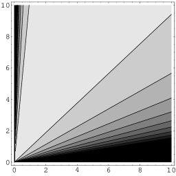
Figure 1: The momentum field (contours of $\psi$ that describe the streamlines of the poloidal component of $\bm{P}$) of the similarity solution (with $D=1$, $p=1$, $J=0.1$ and $q=1$).

The level sets of $\psi$ (hence, those of $\tau$) are the streamlines of $\bm{P}$. On the other hand, $\sigma$ serves as the coordinate directed parallel to the streamlines. We assume that $\rho_{1}$ is written as

$$\rho_{1}(\tau,\sigma)=\rho_{\perp}(\tau)\rho_{\parallel}(\sigma),$$ (29)

and, then, $\log\rho_{1}=\log\rho_{\perp}(\tau)+\log\rho_{\parallel}(\sigma)$.

Let us see how the stream function $\psi$ of equation (28) satisfies equations (21), (22) and (16), i.e., we determine all other fields $I_{2}(\psi)$, $\rho_{1}$, $\rho_{2}$, $\nu$ and $h$ that allow this $\psi$ to be the solution. For arbitrary $f(\tau)$ and $g(\tau)$, we observe

$${\cal L}f=\frac{1}{r^{2}}\left[(\tau^{2}+1)f^{\prime\prime}+3\tau f^{\prime}\right],$$

$$\nabla f\cdot\nabla g=\frac{1}{r^{2}}(\tau^{2}+1)f^{\prime}g^{\prime}.$$

Hence, the left-had side of equation (21) is (denoting $g(\tau)\equiv\log\rho_{\perp}(\tau)$)

$${\cal L}\psi-\nabla\psi\cdot\nabla\log\rho_{1}$$

$$~{}~{}=\frac{1}{r^{2}}\left[(\tau^{2}+1)\psi^{\prime\prime}+3\tau\psi^{\prime}-(\tau^{2}+1)g^{\prime}\psi^{\prime}\right].$$ (30)

For this quantity to balance with the right-hand side of equation (21), which has no explicit dependence on $r^{-2}$, both sides must be zero, i.e., we have to set $I_{2}^{\prime}(\psi)=0$ (the implication of this simple condition will be discussed later). Then, equation (21) reduces to

$$(\tau^{2}+1)\psi^{\prime\prime}+3\tau\psi^{\prime}-(\tau^{2}+1)g^{\prime}\psi^{\prime}=0.$$ (31)

We note that the Beltrami condition (31) is freed from $\rho_{\parallel}(\sigma)$. This fact merits in solving equation (16); see equation (34).

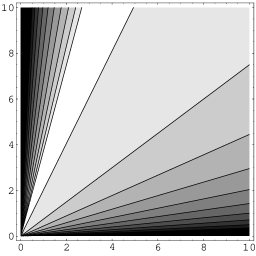
Figure 2: The distribution of $\rho_{\perp}$ of the similarity solution (with $D=1$, $p=1$, $J=0.1$ and $q=1$). Contour curves are given in the log scale of $\rho_{\perp}$.

For the specific form (28) of $\psi$, we have to determine an appropriate $g=\log\rho_{\perp}$ to satisfy equation (31), i.e.,

$$g^{\prime} = \frac{\psi^{\prime\prime}}{\psi^{\prime}}+\frac{3\tau}{\tau^{2}+1}$$ (32)

$$= \frac{J\,p\,(p-1)\tau^{p+q}+D\,q\,(q+1)}{J\,p\,\tau^{p+q+1}-D\,q\,\tau}+\frac{3\tau}{\tau^{2}+1}.$$

Solving equation (32), we obtain

$$g\equiv\log\rho_{\perp}=\log\frac{|Jp\tau^{p+q}-Dq|}{\tau^{q+1}}+\frac{3}{2}\log(\tau^{2}+1),$$

and, thus,

$$\rho_{\perp}=\frac{(\tau^{2}+1)^{3/2}|Jp\tau^{p+q}-Dq|}{\tau^{q+1}}.$$ (33)

In Fig. 2, we show the profile of $\rho_{\perp}(\tau)$.

5.2 Bernoulli relation in the disk region

As mentioned above, this solution assumes $I_{2}^{\prime}(\psi)~{}(=\lambda)=0$, and hence, $I_{2}=\rho_{2}rV_{\theta}$ must uniformly distribute. In the disk region (the vicinity of $z=0$), we may approximate $V_{\theta}\approx\sqrt{MG/r}$ (Keplerian velocity). Hence, $\rho_{2}\propto r^{-1/2}$. In Fig. 3, we show the profile of $\rho=\rho_{1}\rho_{2}$ for the case of $\rho_{1}\propto\rho_{\perp}$ (i.e., $\rho_{\parallel}=$constant).

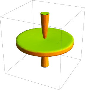
Figure 3: The density $\rho$ in the similarity solution (with $D=1$, $p=1$, $J=0.1$ and $q=1$). We assume $\rho_{\parallel}(\sigma)\approx z^{-2/3}$ and $\rho_{2}\approx r^{-1/2}$. A levelset surface of $\rho$ is shown in the doiman $r<5$ and $|z|<5$.

For $\rho=\rho_{1}\rho_{2}=\rho_{\parallel}\rho_{\perp}r^{-1/2}$, equation (16) reads as

$$\nu=\frac{-d\psi/dz}{2\rho_{\parallel}\rho_{\perp}}r^{-3/2}\propto\frac{r^{-5/2}}{\rho_{\parallel}(r)}$$ (34)

along each streamline in the disk region. For a given $\nu$, we can solve equation (34) for $\rho_{\parallel}$ to determine the density profile.

In the disk region the Bernoulli relation (14) accounts as follows: by $\nabla\cdot\bm{P}=0$, we have $P_{r}=\rho V_{r}\propto r^{-1}$. If $\rho_{\parallel}(\sigma)=$ constant, for example, $\rho\propto r^{-1/2}$ (evaluated along a streamline in the disk region). Then, we have $V_{r}=V_{r0}r^{-1/2}$ with a (negative) constant $V_{r0}$. Combining the azimuthal velocity $V_{\theta}=V_{\theta 0}r^{-1/2}$ (which must be slightly smaller than the Keplerian velocity $\sqrt{MG/r}$), we obtain

$$V^{2}=(V_{r0}^{2}+V_{\theta 0}^{2})r^{-1}=V_{0}^{2}r^{-1}.$$

By $\rho_{2}\propto r^{-1/2}$, we obtain $\partial_{r}(\log\rho_{2})=-(1/2)r^{-1}$. Hence, the Bernoulli relation (14) demands

$$\partial_{r}h=(V_{0}^{2}-MG)r^{-2},$$

which yields $h=(MG-V_{0}^{2})r^{-1}$. In this estimate, all components of the energy density (gravitational potential $\phi$, kinetic energy $V^{2}/2$ and enthalpy $h$) have a similar profile ($\propto r^{-1}$).

5.3 Bernoulli relation in the jet region

In the jet region (vicinity of $r=0$), the streamlines (contours of $\tau=z/r$) are almost vertical, and we may approximate $\sigma\approx z$.

Let us first estimate $\rho_{2}$ using equation (16), which is approximated, in the jet region, by

$$r\rho\nu = \{\log\rho_{2},\psi\}$$ (35)

$$\approx (\partial_{r}\psi)\,(\partial_{z}\log\rho_{2})$$

$$= J\,p\,\tau^{p+1}\frac{1}{z}\,\partial_{z}(\log\rho_{2}),$$

which shows that $\rho_{2}$ is an increasing function of $|z|$. Using $\rho=\rho_{\parallel}(\sigma)\rho_{\perp}(\tau)\rho_{2}$, we integrate equation (35) along the streamline ($\tau=$constant, $\sigma\approx z$):

$$\frac{d\rho_{2}}{\rho_{2}^{2}}=-d\left(\frac{1}{\rho_{2}}\right)=\frac{\nu}{Jp}\ \tau^{p+2}\,\rho_{\perp}(\tau)\rho_{\parallel}(z)z^{2}dz.$$ (36)

With this $\rho_{2}(z)$, we may estimate the toroidal (azimuthal) component of the velocity: $V_{\theta}=I_{2}/(r\rho_{2})=(I_{2}\tau)/(z\rho_{2})$, where $I_{2}$ and $\tau$ are constant (the latter is constant along each streamline). We find that the kinetic energy $V_{\theta}^{2}/2$ of the azimuthal velocity decreases as a function of $|z|$ (both by the geometric expansion factor $z^{-2}$ and the friction damping effect $\rho_{2}^{-2}$). The steep gradient of the corresponding hydrodynamic pressure yields a strong boost near the foot point ($z\approx 0$).

The poloidal component of the kinetic energy is estimated as follows: We may approximate

$$\frac{1}{2}(V_{r}^{2}+V_{z}^{2}) = \frac{1}{2\rho^{2}r^{2}}\,|\nabla\psi|^{2}$$ (37)

$$\approx \frac{1}{2\rho^{2}r^{2}}\left(Jp\frac{z^{p}}{r^{p+1}}\right)^{2}$$

$$= \frac{(Jp)^{2}\tau^{2p+4}}{2\rho^{2}z^{4}}.$$

Here, the vertical distribution of the density $\rho=\rho_{\perp}(\tau)\rho_{\parallel}(\sigma)\rho_{2}$ is primarily dominated by $\rho_{\parallel}(\sigma)\approx\rho_{\parallel}(z)$.

At long distance from the origin, the jet has a natural similarity property. For simplicity, let us ignore the effect of the friction ($\nu=0$), and assume $\rho_{2}=1$. Then, $\rho_{\parallel}\propto|z|^{-3/2}$ yields $(V_{r}^{2}+V_{z}^{2})/2\propto z^{-1}$, which may balance with the gravitational potential energy $\phi=-MG|z|^{-1}$. Note, that the azimuthal component of the kinetic energy disappears at large scale ($V_{\theta}^{2}\propto z^{-2}$). The Bernoulli condition (14) gives $h$ that also has a similar distribution of $\propto|z|^{-1}$.

In Fig. 3, we show the profile of $\rho=\rho_{\perp}\rho_{\parallel}\rho_{2}$ with $\rho_{\parallel}\propto|z|^{-3/2}$ (jet region) and $\rho_{2}\propto r^{-1/2}$ (disk region).

6 Summary and Concluding Remarks

We have shown that the combination of a thin disk and narrowly-collimated jet is the unique structure that is amenable to the singularity of the Keplerian vorticity; the Beltrami condition, imposing the alignment of flow and generalized vorticity, characterizes such a geometry. Here the conventional vorticity is generalized to combine with magnetic field (or, electromagnetic vorticity) as well as to subtract the friction force causing the accretion.

In Section 5, we have given an analytic solution in which the generalized vorticity is purely kinematic ($\bm{\Omega}=\nabla\times\bm{P}_{2}$ with the momentum $\bm{P}_{2}$ that is modified by the friction effect). The principal force that ejects the jet is, then, the hydrodynamic pressure dominated by $V_{\theta}^{2}/2$. Additional magnetic force may contribute to jet acceleration if the self-consistently generated large-scale magnetic field is sufficiently large [18, 35, 37, 41, 42]. Such structures can be described by the generalized model of Subsection 4.1.

The similarity solution has a singularity at the origin (where the model gravity $\phi=-MGr^{-1}$ is singular), which disconnects the disk part (parameterized by $D$ and $q$) and the jet part (parameterized by $J$ and $p$). To “connect” both subsystems (or, to relate $D$, $q$, $J$, and $p$), we need a singular perturbation that dominates the small-scale hierarchy [44]. The connection point must switch the topology of the flow: In the poloidal cross section, the streamlines of the mass flow, which connect the accreting inflow and jet’s outflow, describe hyperbolic curves converging to the radial and the vertical axes. On the other hand, the vorticity lines (or generalized magnetic field lines) thread the disk. This topological difference of these two vector fields demands “decoupling” of them. Instead of disconnecting them by a singularity, we will have to consider a small-scale structure in which the topological switch can occur [40]. The Hall effect (scaled by $\epsilon$) or the viscosity/resistivity (scaled by reciprocal Reynolds number) yields a singular perturbation (then, the generalized magneto-Bernoulli mechanism [33, 34] may effectively accelerate the jet-flow). In a weakly ionized plasma, the electron equation (2) is modified so that the Hall effect is magnified by the ratio of the neutral and electron densities; the ambipoler diffusion effect also yields a higher-order perturbation [24]. The mechanism of singular perturbation and the local structure of the disk-jet connection point may differ depending on the plasma condition near the central object: in AGN, the plasma is fully ionized but rather collisional (we also need a relativistic equation of state with possible presence of pairs), and, in YSO, the plasma is partially ionized; the relevant dissipation mechanisms determine the scale hierarchy in the vicinity of the singularity. The study of above concrete cases was not the scope of present paper and will be considered elsewhere. Our goal was to show how the alignment of flow and generalized vorticity condition arises and how it determines the singular structure of a thin disk and narrowly-collimated jet invoking the simplest (minimum) model of magnetohydrodynamics.

References

References

- [1] Anderson J M, Li Z Y, Krasnopolsky R and Blandford R D 2005 The Structure of Magnetocentrifugal Winds. I. Steady Mass Loading ApJ 630 945
- [2] Balbus S A and Hawley J F 1998 Instability, turbulence, and enhanced transport in accretion disks Rev. Mod. Phys. 70 1
- [3] Begelman M C, Blandford R D and Rees M J 1984 Theory of extragalactic radio sources Rev. Mod. Phys. 56 255
- [4] Begelman M C 1993 Conference summary Astrophysical Jets ed D Burgarella et al (Cambridge: Cambridge Univ. Press) pp. 305-315
- [5] Begelman M C 1998 Instability of Toroidal Magnetic Field in Jets and Plerions ApJ 493 291
- [6] Blandford R D and Rees M J 1974 A ’twin-exhaust’ model for double radio sources MNRAS 169 395
- [7] Blandford R D and Znajek R L 1977 Electromagnetic extraction of energy from Kerr black holes MNRAS 179 433
- [8] Blandford R D and Payne D G 1982 Hydromagnetic flows from accretion discs and the production of radio jets MNRAS 199 883
- [9] Blandford R D 1994 Particle acceleration mechanisms ApJS 90 515
- [10] Bogovalov S V and Kelner S R 2010 Accretion and Plasma Outflow from Dissipationless Discs IJMP D 19 339
- [11] Chandrasekhar S 1956 On Force-Free Magnetic Fields Proc. Natl. Acad. Sci. USA 42 1
- [12] Celotti A and Blandford R D 2001 Black Holes in Binaries and Galactic Nuclei: Diagnostics, Demography and Formation ESO Astrophysics Symposia ed L Kaper et al (Berlin, Heidelberg: Springer-Verlag), 206
- [13] Ferrari A 1998 Modeling Extragalactic Jets Annu. Rev. Astron. Astrophys. 36 539
- [14] Ferreira J 1997 Magnetically-driven jets from Keplerian accretion discs A&A 319 340
- [15] Ferreira J, Dougados C and Cabrit S 2006 Which jet launching mechanism(s) in T Tauri stars? A&A 453 785
- [16] Ferreira J, Dougados C and Whelan E 2007 Jets from Young Stars I: Models and Constraints Lecture Notes in Physics ed J Ferreira et al (Berlin, Heidelberg: Springer-Verlag) 723 181
- [17] Hartigan P, Edwards S and Ghandour L 1995 Disk Accretion and Mass Loss from Young Stars ApJ 452 736
- [18] Hawley J F, Gammie C F and Balbus S A 1995 Local Three-dimensional Magnetohydrodynamic Simulations of Accretion Disks ApJ 440 742
- [19] Heinz S and Begelman M C 2000 Jet Acceleration by Tangled Magnetic Fields ApJ 535 104
- [20] Jones D L, Werhle A E, Meier D L and Piner B G 2000 The Radio Jets and Accretion Disk in NGC 4261 ApJ 534 165
- [21] Königl A and Pudritz R E 2000 Disk Winds and the Accretion-Outflow Connection Protostars and Planets IV ed V Mannings et al (Tuscon: Univ. Arizona Press) 759
- [22] Krasnopolsky R, Li Z Y and Blandford R D 1999 Magnetocentrifugal Launching of Jets from Accretion Disks. I. Cold Axisymmetric Flows ApJ 526 631
- [23] Krasnopolsky R, Li Z Y and Blandford R D 2003 Magnetocentrifugal Launching of Jets from Accretion Disks II. Inner Disk-driven Winds ApJ 595 631
- [24] Krishan V and Yoshida Z 2009 Kolmogorov dissipation scales in weakly ionized plasmas MNRAS 395 2039
- [25] Kudoh T and Shibata K 1997 Magnetically Driven Jets from Accretion Disks. I. Steady Solutions and Application to Jets/Winds in Young Stellar Objects ApJ 474 362
- [26] Kudoh T, Matsumoto R and Shibata K 2003 MHD simulations of jets from accretion disks Astrophys. Sp. Sci. 287 99
- [27] Kuwabara T, Shibata K, Kudoh T and Matsumoto R 2005 The Acceleration Mechanism of Resistive Magnetohydrodynamic Jets Launched from Accretion Disks ApJ 621 921
- [28] Livio M 1997 The Formation Of Astrophysical Jets Accretion Phenomena and Related Outflows; IAU Colloquium 163 ed. D T Wickramasinghe et al (San Francisco: ASP) ASP Conference Series 121 845
- [29] Livio M., 1999, Phys. Rep., 311, 225
- [30] Low B C 1982 Nonlinear force-free magnetic fields Rev. Geophys. Space Phys. 20 145
- [31] Machida M and Matsumoto R 2003 Global Three-dimensional Magnetohydrodynamic Simulations of Black Hole Accretion Disks: X-Ray Flares in the Plunging Region ApJ 585 429
- [32] Mahajan S M and Yoshida Z 1998 Double Curl Beltrami Flow: Diamagnetic Structures Phys. Rev. Lett. 81 4863
- [33] Mahajan S M, Nikol’skaya K I, Shatashvili N L and Yoshida Z 2002 Generation of Flows in the Solar Atmosphere Due to Magnetofluid Coupling ApJ 576 L161
- [34] Mahajan S M, Shatashvili N L, Mikeladze S V and Sigua K I 2006 Acceleration of plasma flows in the closed magnetic fields: Simulation and analysis Phys. Plasmas 13 062902
- [35] Matsumoto R and Tajima T 1995 Magnetic viscosity by localized shear flow instability in magnetized ApJ 445 767
- [36] Matsumoto R, Machida M and Nakamura K 2004 Global 3D MHD Simulations of Optically Thin Black Hole Accretion Disks Prog. Theor. Phys. Suppl. 155 124
- [37] Ogilvie G I and Livio M 1998 On the Difficulty of Launching an Outflow from an Accretion Disk ApJ 499 329
- [38] Pelletier G and Pudritz R E 1992 Hydromagnetic disk winds in young stellar objects and active galactic nuclei ApJ 394 117
- [39] Shakura N I and Sunyaev R 1973 Black holes in binary systems. Observational appearance A&A 24 337
- [40] Shiraishi J, Yoshida Z and Furukawa M 2009 Topological Transition from Accretion to Ejection in a Disk-Jet System - Singular Perturbation of the Hall Effect in a Weakly Ionized Plasma ApJ 697 100
- [41] Tout C A and Pringle J E 1996 Can a disc dynamo generate large-scale magnetic fields? MNRAS 281 219
- [42] Vlemmings W H T, Bignall H E and Diamond P J 2007 Green Bank Telescope Observations of the Water Masers of NGC 3079: Accretion Disk Magnetic Field and Maser Scintillation ApJ 656 198
- [43] Yoshida Z and Giga Y 1990 Remarks on spectra of operator ROT Math. Z. 204 235
- [44] Yoshida Z, Mahajan S M and Ohsaki S 2004 Scale hierarchy created in plasma flow Phys. Plasmas 11 3660
- [45] Yoshida Z 2009 Clebsch parameterization: Basic properties and remarks on its applications J. Math. Phys. 50 113101
- [46] Zanni C, Ferrari A, Rosner R, Bodo G and Massaglia S 2007 MHD simulations of jet acceleration from Keplerian accretion disks. The effects of disk resistivity A&A 469 811