A Comparison between a Minijet Model and a Glasma Flux Tube Model for Central Au-Au Collisions at $\sqrt{s_{NN}}$=200 GeV.

Abstract

In is paper we compare two models with central Au-Au collisions at $\sqrt{s_{NN}}$=200 GeV. The first model is a minijet model which assumes that around $\sim$50 minijets are produced in back-to-back pairs and have an altered fragmentation functions. It is also assumed that the fragments are transparent and escape the collision zone and are detected. The second model is a glasma flux tube model which leads to flux tubes on the surface of a radial expanding fireball driven by interacting flux tubes near the center of the fireball through plasma instabilities. This internal fireball becomes an opaque hydro fluid which pushes the surface flux tubes outward. Around $\sim$12 surface flux tubes remain and fragment with $\sim$1/2 the produced particles escaping the collision zone and are detected. Both models can reproduce two particle angular correlations in the different $p_{t1}$ $p_{t2}$ bins. We also compare the two models for three additional effects: meson baryon ratios; the long range nearside correlation called the ridge; and the so-called mach cone effect when applied to three particle angular correlations.

I Introduction and review of models

In this paper we discuss two models. The first model is a minijet modelTrainor1 . The second is a glasma flux tube model (GFTM)Dumitru .

The paper is organized in the following manner:

Sec. 1 is the introduction and review of models. Sec. 2 discuss two particle angular correlation in the two models. Sec. 3 discuss baryon and anti-baryon formation in both models. Sec. 4 demonstrates how the ridge is formed by flux tubes when a jet trigger is added to the GFTM. Sec. 5 treats the so-called mach cone effect by analyzing three particle angular correlations in the two models. Sec. 6 presents the summary and discussion.

I.1 Minijet Model

The analysis of angular correlations led to unanticipated structure in the final state of p-p and Au-Au collisions, subsequently identified with parton fragmentation in the form of minijets[3-7]. Two-component analysis of p-p and Au-Au spectra revealed a corresponding hard component, a minimum-bias fragment distribution associated with minijets, suggesting that jet phenomena extend down to 0.1 GeV/cTrainor2 ; star4 . From a given p-p or Au-Au collisions particles are produced with three kinematic variables ($\eta$,$\phi$,$p_{t}$). The $p_{t}$ spectra provide information about parton fragmentation, but the fragmentation process is more accessible on a logarithmic momentum variable. The dominant hadron (pion) is ultrarelativistic at 1 GeV/c, and a relativistic kinematic variable is a reasonable alternative. Transverse rapidity in a longitudinally comoving frame near midrapidity $\eta$=0 is defined by

$$y_{t}=ln([m_{t}+p_{t}]/m_{0}),$$ (1)

with $m_{0}$ a hadron mass and $m_{t}^{2}$ = $p_{t}^{2}$ + $m_{0}^{2}$. If one integrates over $\phi$ the event multiplicity ($dn/d\eta$ $\equiv$ $\rho$, the 1D density on $\eta$) can be written for p-p collision in a two component model as

$$\rho(y_{t};\eta=0)=S_{0}(y_{t})+H_{0}(y_{t}).$$ (2)

$S_{0}$ is a Levy distribution on $m_{t}$ which represents soft processes and $H_{0}$ is a Gaussian on $y_{t}$ which represents hard processes. The soft process has no $\phi$ dependence but does have a Gaussian correlation in the longitudinal direction($\eta$). This correlation can be expressed in a two particle way as $\Delta\eta=\eta_{1}-\eta_{2}$ which is the difference of the psuedorapidity.

$$\rho_{s}(\Delta\eta)=A_{0}exp[-\Delta\eta^{2}/2\sigma_{0}^{2}].$$ (3)

The hard process arise from a scattering of two partons thus minijets are formed. Each minijet fragments along its parton axis and generates a 2D correlation $\Delta\phi=\phi_{1}-\phi_{2}$ and $\Delta\eta=\eta_{1}-\eta_{2}$.

$$\rho_{h}(\Delta\phi,\Delta\eta)=A_{h}exp[-\Delta\phi^{2}/2\sigma_{\phi}^{2}]exp[-\Delta\eta^{2}/2\sigma_{\eta}^{2}].$$ (4)

Since for every minijet fragmenting leading to a peak at $\Delta\phi$ = $0^{\circ}$, there is its scattered partner in the backward direction $\Delta\phi$ = $180^{\circ}$. The backward scattered minijet will range over many psuedorapidity values, therefore its correlation with the fragmentation of the near side minijet will have a broad $\Delta\eta$ width. In this condition simple momentum conservation is good enough and that is a $-cos(\Delta\phi)$ term.

The two-component model of hadron production in A-A collisions assumes that the soft component is proportional to the participant pair number (linear superposition of N-N collisions), and the hard component is proportional to the number of N-N binary collisions (parton scattering)Nardi . Any deviations from the model are specific to A-A collisions and may reveal properties of an A-A medium. In terms of mean participant path length $\nu$ = 2$n_{bin}$/$n_{part}$ the $p_{t}$-integrated A-A hadron density on $\eta$ is

$${2\over n_{part}}{dn\over d\eta_{AA}}=\rho_{s}+\nu\rho_{h}.$$ (5)

By analogy with Eg. (2) A-A density as a function of centrality parameter $\nu$ becomes

$${2\over n_{part}}\rho_{AA}(y_{t};\nu,\eta=0)=S_{NN}(y_{t})+\nu r_{AA}(y_{t};\nu)H_{NN}(y_{t}).$$ (6)

In the above equation $S_{NN}(y_{t})$ = $S_{0}(y_{t})$ and $H_{NN}(y_{t})$ = $H_{0}(y_{t})$ which is p-p scattering or nucleon-nucleon scattering. We also can define for the hard density for A-A collisions in terms of $\nu$ as $H_{AA}(y_{t};\nu)$ = $r_{AA}(y_{t};\nu)H_{NN}(y_{t})$. The density 2/$n_{part}$ 1/2$\pi$ 1/$y_{t}$ $d^{2}$/$dy_{t}$$d\eta$ for pions as a function of $y_{t}$ at $\sqrt{s_{NN}}$=200 GeV for p-p, Au-Au, and $H_{NN}(y_{t})$ is shown in Figure 1.

Figure 1: Pion $y_{t}$ density for five Au-Au centralities (solid curves). Density for p-p is also shown (solid dots). $H_{NN}$ is the hard Gaussian on $y_{t}$ which represents hard processes (dash-dot curve).

We see from the above equation the $S_{NN}(y_{t})$ is universal and scales with the participant pairs. This means we can extract $\nu H_{AA}(y_{t})$ from the density measured in p-p and Au-Au at $\sqrt{s_{NN}}$=200 GeV from Figure 1 giving us Figure 2.

Figure 2: The hard component of pion $y_{t}$ spectra in the form $\nu H_{AA}(y_{t})$ (thicker curves with changing line style) compared to two-component reference $\nu H_{NN}(y_{t})$ (dotted curve). The dashed reference curves are limiting cases for $\nu$ = 1, 6.

Finally the ratio $H_{AA}$/$H_{NN}$ ($R_{AA}$) is plotted in Figure 3. In the Au-Au central collision (0-12%) at a $y_{t}$ value of 2 ($p_{t}$=0.5 GeV/c) there is 5 times as many pions coming from minijet fragmentation as there is in a N-N collision. This implies a large increase in correlated pion fragments and should show up as an increased in two particle angular correlations. We will see this in Sec. 2 where we show these angular correlations and discuss the number of particles in the minijets.

Figure 3: Hard-component ratio for pions and five Au-Au centralities (thicker curves with changing line styles) relative to the N-N hard-component reference. The connected dots are data from NSD p-p collisions.

The common measurement of parton energy loss is expressed as a nuclear modification factor $R_{AA}$. The hard-component ratio $r_{AA}$ measured over $y_{t}$ ($p_{t}$) provides similar information. Note that $y_{t}$ = 5 ($p_{t}$=10 GeV/c) $r_{AA}$ = 0.2 which is the same value calculated for $R_{AA}$. This value is considered caused by jet quenching as partons are absorbed by the opaque medium. However in the minijet picture suggests that no partons are lost in A-A collisions. Their manifestation (in spectrum structure and correlations) is simply redistributed within the fragment momentum distribution, and the fragment number increases. A high-$p_{t}$ triggered jet yield may be reduced by a factor of five within a particular $p_{t}$ range, but additional fragments emerge elsewhere, still with jet-like correlation structurestar1 ; star2 ; Kettler .

I.2 Glasma Flux Tube Model

A glasma flux tube model (GFTM)Dumitru that had been developed considers that the wavefunctions of the incoming projectiles, form sheets of color glass condensates (CGC)CGC that at high energies collide, interact, and evolve into high intensity color electric and magnetic fields. This collection of primordial fields is the GlasmaLappi ; Gelis , and initially it is composed of only rapidity independent longitudinal color electric and magnetic fields. An essential feature of the Glasma is that the fields are localized in the transverse space of the collision zone with a size of 1/$Q_{s}$. $Q_{s}$ is the saturation momentum of partons in the nuclear wavefunction. These longitudinal color electric and magnetic fields generate topological Chern-Simons chargeSimons which becomes a source for particle production.

The transverse space is filled with flux tubes of large longitudinal extent but small transverse size $\sim$$Q^{-1}_{s}$. Particle production from a flux tube is a Poisson process, since the flux tube is a coherent state. The flux tubes at the center of the transverse plane interact with each other through plasma instabilitiesLappi ; Romatschke1 and create a locally thermalized system, where partons emitted from these flux tubes locally equilibrate. A hydro system with transverse flow builds causing a radially flowing blast waveGavin . The flux tubes that are near the surface of the fireball get the largest radial flow and are emitted from the surface.

$Q_{s}$ is around 1 GeV/c thus the transverse size of the flux tube is about 1/4fm. The flux tubes near the surface are initially at a radius $\sim$5fm. The $\phi$ angle wedge of the flux tube is $\sim$1/20 radians or $\sim$$3^{\circ}$. Thus the flux tube initially has a narrow range in $\phi$. The width in $\Delta\eta$ correlation of particles results from the independent longitudinal color electric and magnetic fields that created the Glasma flux tubes. In this paper we relate particle production from the surface flux tube to a related model Parton Bubble Model(PBM)PBM . It was shown in Ref.PBMGFTM that for central Au-Au collisions at $\sqrt{s_{NN}}$=200 the PBM is a good approximation to the GFTM surface flux tube formation.

The flux tubes on the surface turn out to be on the average 12 in number. They form an approximate ring about the center of the collision see Figure 4. The twelve tube ring creates the average behavior of tube survival near the surface of the expanding fire ball of the blast wave. The final state surface tubes that emit the final state particles at kinetic freezeout are given by the PBM. One should note that the blast wave surface is moving at its maximum velocity at freezeout (3c/4).

Figure 4: The tube geometry is an 8 fm radius ring perpendicular to and centered on the beam axis. It is composed of twelve adjacent 2 fm radius circular tubes elongated along the beam direction as part of the flux tube geometry. We project on a plane section perpendicular to the beam axis.

The space momentum correlation of the blast wave provides us with a strong angular correlation signal. PYTHIA fragmentation functionspythia were used for the tube fragmentation that generate the final state particles emitted from the tube. The initial transverse size of a flux tube $\sim$1/4fm has expanded to the size of $\sim$2fm at kinetic freezeout. Many particles that come from the surface of the fireball will have a $p_{t}$ greater than 0.8 Gev/c. The final state tube size and the Hanbury-Brown and Twiss (HBT) observationsHBT of pions that have a momentum range greater than 0.8 GeV/c are consistent both being $\sim$2fm. A single parton using PYTHIA forms a jet with the parton having a fixed $\eta$ and $\phi$ (see Figure 5). For central events each of the twelve tubes have 3-4 partons per tube each at a fixed $\phi$ for a given tube. The $p_{t}$ distribution of the partons is similar to pQCD but has a suppression at high $p_{t}$ like the data. The 3-4 partons in the tube which shower using PYTHIA all have a different $\eta$ values but all have the same $\phi$ (see Figure 6). The PBM explained the high precision Au-Au central (0-10%) collisions at $\sqrt{s_{NN}}=$ 200 GeVcentralproduction (the highest RHIC energy).

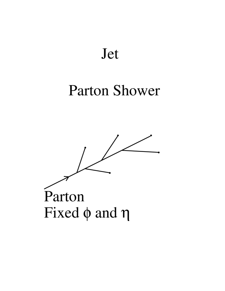
Figure 5: A jet parton shower.

Figure 6: Each tube contains 3-4 partons as shown.

II The Correlation Function for Central Au-Au Data

We utilize a two particle correlation function in the two dimensional (2-D) space of $\Delta\phi$ versus $\Delta\eta$. The 2-D total correlation function is defined as:

$$C(\Delta\phi,\Delta\eta)=S(\Delta\phi,\Delta\eta)/M(\Delta\phi,\Delta\eta).$$ (7)

Where S($\Delta\phi,\Delta\eta$) is the number of pairs at the corresponding values of $\Delta\phi,\Delta\eta$ coming from the same event, after we have summed over all the events. M($\Delta\phi,\Delta\eta$) is the number of pairs at the corresponding values of $\Delta\phi,\Delta\eta$ coming from the mixed events, after we have summed over all our created mixed events. A mixed event pair has each of the two particles chosen from a different event. We make on the order of ten times the number of mixed events as real events. We rescale the number of pairs in the mixed events to be equal to the number of pairs in the real events. This procedure implies a binning in order to deal with finite statistics. The division by M($\Delta\phi,\Delta\eta$) for experimental data essentially removes or drastically reduces acceptance and instrumental effects. If the mixed pair distribution was the same as the real pair distribution C($\Delta\phi,\Delta\eta$) should have unit value for all of the binned $\Delta\phi,\Delta\eta$. In the correlations used in this paper we select particles independent of its charge. The correlation of this type is called a Charge Independent (CI) Correlation. This difference correlation function has the defined property that it only depends on the differences of the azimuthal angle ($\Delta\phi$) and the beam angle ($\Delta\eta$) for the two particle pair. Thus the two dimensional difference correlation distribution for each tube or minijet which is part of C($\Delta\phi,\Delta\eta$) is similar for each of the objects and will image on top of each other. We further divide the data (see Table I) into $p_{t}$ ranges (bins).

$p_{t}$ range	amount
$4.0GeV/c-1.1GeV/c$	149
$1.1GeV/c-0.8GeV/c$	171
$0.8GeV/c-0.65GeV/c$	152
$0.65GeV/c-0.5GeV/c$	230
$0.5GeV/c-0.4GeV/c$	208
$0.4GeV/c-0.3GeV/c$	260
$0.3GeV/c-0.2GeV/c$	291

Table 1: The $p_{t}$ bins and the number of charged particles per bin with $|\eta|$ $<$ 1.0.

Since we are choosing particle pairs, we choose for the first particle $p_{t1}$ which could be in one bin and for the second particle $p_{t2}$ which could be in another bin. Therefore binning implies a matrix of $p_{t1}$ vs $p_{t2}$. We have have 7 bins thus there are 28 independent combinations. Each of the combinations will have a different number of enters. In order to take out this difference one uses multiplicity scalingPBME ; centralitydependence . The diagonal bins one scales event average of Table I. For the off diagonal combinations one uses the product of square root of corresponding diagonal event averages. In Figure 7 we show the correlation function equation 7 for the highest diagonal bin $p_{t}$ 4.0 to 1.1 GeV/c. Figure 8 is the smallest diagonal bin $p_{t}$ 0.3 to 0.2 GeV/c.

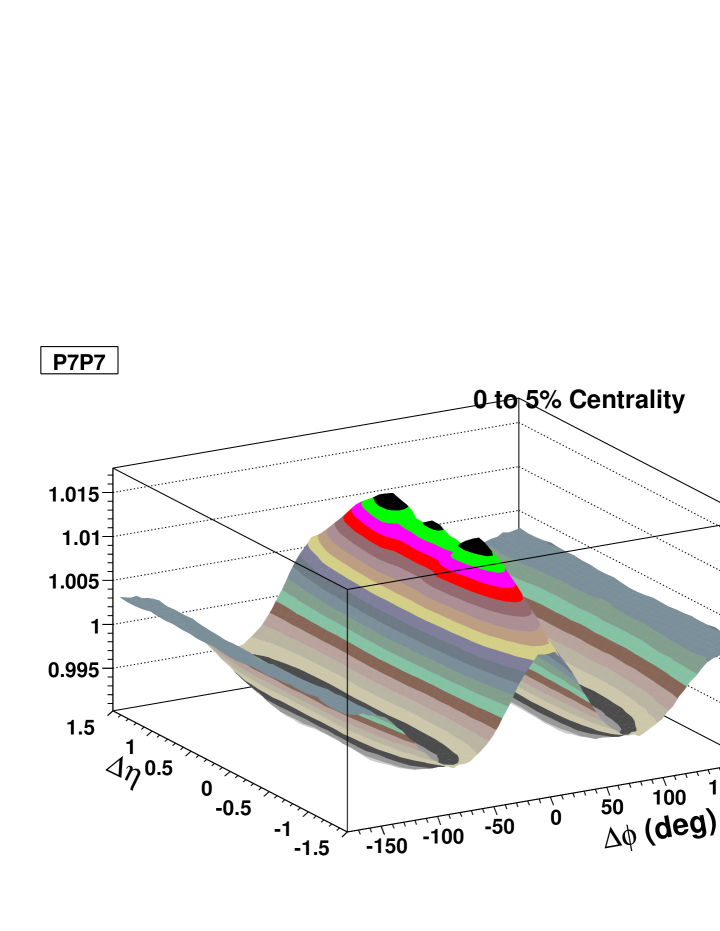
Figure 7: $\Delta\phi$ vs.$\Delta\eta$ CI correlation for the 0-5% centrality bin for Au-Au collisions at $\sqrt{s_{NN}}=$ 200 GeV requiring both particles to be in bin 7 $p_{t}$ greater than 1.1 GeV/c and $p_{t}$ less than 4.0 GeV/c.

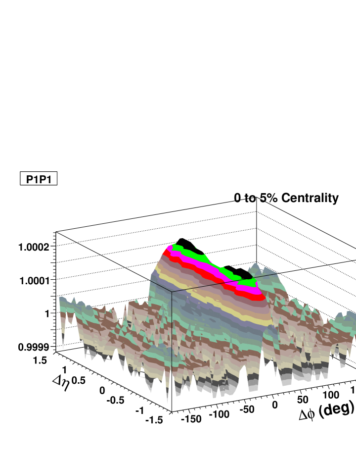
Figure 8: $\Delta\phi$ vs.$\Delta\eta$ CI correlation for the 0-5% centrality bin for Au-Au collisions at $\sqrt{s_{NN}}=$ 200 GeV requiring both particles to be in bin 1 $p_{t}$ greater than 0.2 GeV/cand $p_{t}$ less than 0.3 GeV/c.

Once we use multiplicity scaling we can compare all 28 combinations. In Figure 9 we show the 28 plots all having the same scale. This make it easy to see how fast the correlation signals drop off with lowering the momentum. These plots show the properties of parton fragmentation. P1P7 has the same signal as P2P6, P3P5, and P4P4. It should be noted that both the minijet model and GFTM give the same two particle correlations.

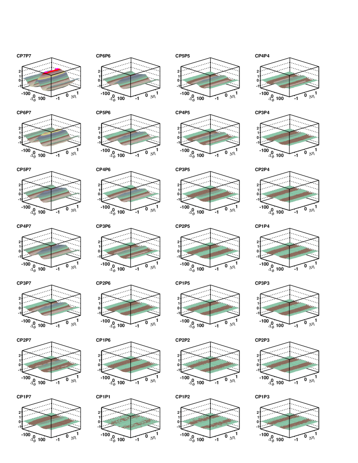
Figure 9: $\Delta\phi$ vs.$\Delta\eta$ CI correlation for the 0-5% centrality bin for Au-Au collisions at $\sqrt{s_{NN}}=$ 200 GeV for all 28 combination of $p_{t1}$ vs $p_{t2}$ not rescaled (see text).

II.1 The properties of the minijet model

For the above correlations on average there was 48 minijets per central Au-Au collision. Each minijet on the average showered into 13 charged particles. The soft uncorrelated particles accounted for 837 or 57% of the charged particles. This means that 43% of the charged particles come from minijet fragmentation (see Table II). All of the particles coming from minijet fragmentation add toward the final observed correlation signal with none being absorbed. The fact that the spectrum has been soften and spread out in the beam direction ($\eta$), is a medium modification which has not been yet calculated using QCD.

variable	amount	fluctuations
$minijets$	48	4
$particles$	13	4
$soft$	837	29

Table 2: Parameters of the minijet model for charged particles.

II.2 The properties of the Glasma Flux Tube Model

For the above correlations on average there was 12 final state tubes on the surface of the fireball per central Au-Au collision. Each tube on the average showered into 49 charged particles. The soft uncorrelated particles accounted for 873 or 60% of the charged particles. Since the tubes are sitting on the surface of the fireball and being push outward by radial flow, not all particles emitted from the tube will escape. Approximately one half of the particles that are on the outward surface leave the fireball and the other half are absorbed by the fireball (see Figure 10). This means that 20% of the charged particles come from tube emission, and 294 particles are added to the soft particles increasing the number to 1167 (see Table III).

Figure 10: Since the tubes are sitting on the surface of the fireball and being push outward by radial flow, not all particles emitted from the tube will escape. Approximately one half of the particles that are on the outward surface leave the fireball and the other half are absorbed by the fireball.

variable	amount	fluctuations
$tubes$	12	0
$particles$	24.5	5
$soft$	1167	34

Table 3: Parameters of the GFTM for charged particles.

The particles that emitted outward are boosted in momentum, while the inward particles are absorbed by the fireball. Out of the initial 49 particles per tube the lower $p_{t}$ particles have larger losses. In Table IV we give a detailed account of these percentage losses and give the average number of charged particles coming from each tube for each $p_{t}$ bin.

$p_{t}$	amount	%survive
$4.0GeV/c-1.1GeV/c$	4.2	100
$1.1GeV/c-0.8GeV/c$	3.8	76
$0.8GeV/c-0.65GeV/c$	3.2	65
$0.65GeV/c-0.5GeV/c$	4.2	54
$0.5GeV/c-0.4GeV/c$	3.2	43
$0.4GeV/c-0.3GeV/c$	3.3	35
$0.3GeV/c-0.2GeV/c$	2.6	25

Table 4: Parameters of the GFTM for $p_{t}$ of the charged particles.

In the surface GFTM we have thermalization and hydro flow for the soft particles, while all the two particle angular correlations come from the tubes on the surface. The charge particle spectrum of the GFTM is given by a blastwave model and the direct tube fragmentation is only 20% of this spectrum. The initial anisotropic azimuthal distribution of flux tubes is transported to the final state leaving its pattern on the ring of final state flux tubes on the surface. This final state anisotropic flow pattern can be decomposed in a Fourier series ($v_{1}$, $v_{2}$, $v_{3}$, …). These coefficients have been measureAlver and have been found to be important in central Au-Au collisions. We will come back to these terms later on when we consider three particle angular correlations.

III Formation of baryon and anti-baryon in both models

It was shown above that charged particle production differ between p-p and Au-Au at $\sqrt{s_{NN}}=$ 200. High $p_{t}$ charged particles in Au-Au are suppressed compared to p-p for $p_{t}$ $>$ 2.0 GeV/c ($y_{t}$ $>$ 3.33 for pions). Figure 3 shows $r_{AA}$ for pions which has a suppression starting at $y_{t}$ = 3.0 ($p_{t}$ = 1.5 GeV/c). This shift between suppression of charged particle at $p_{t}$ $>$ 2.0 GeV/c and suppression of pions at $p_{t}$ = 1.5 GeV/c is made up by an enhancement of baryonsAdler . Proton $r_{AA}$ (see Figure 12) which is the most numerous baryon shows an enhancement starting at $p_{t}$ $>$ 1.5. This enhancement continues to $p_{t}$ = 4.0 ($y_{t}$ = 4.0). Finally at $p_{t}$=10.0 GeV/c ($y_{t}$ = 5.0) $r_{AA}$ = 0.2 which is the same value as pions.

Figure 11: Hard-component ratio for protons and five Au-Au centralities (thicker curves with changing line styles) relative to the N-N hard-component reference. The features are only comparable to Figure 3 for 60-80% or $y_{t}$ $>$ 4.5. Note $y_{t}$ is calculated using a pion mass.

III.1 Minijet Model

There is no a priori model for the proton hard component. The excess in the proton hard component appears anomalous, but may be simply explained in terms of parton energy lossTrainor2 .

III.2 Glasma Flux Tube Model

We have shown previously that inside the tube there are three to four partons with differing longitudinal momenta all at the same $\phi$. The $p_{t}$ distribution of the partons inside the tube is similar to pQCD but has a suppression in the high $p_{t}$ region like the data. The partons which are mainly gluons shower into more gluons which then fragment into quarks and anti-quarks which overlap in space and time with other quarks and anti-quarks from other partons. This leads to an enhance possibility for pairs of quarks from two different fragmenting partons to form a di-quark, since the recombining partons are localized together in a small volume. The same process will happen for pairs of anti-quarks forming a di-anti-quark. This recombination process becomes an important possibility in the GFTM compared to regular jet fragmentation. Since the quarks which overlap have similar phase space, the momentum of the di-quark is approximately twice the momentum of the quarks, but has approximately the same velocity. When mesons are formed quarks pick up anti-quarks with similar phase space from fragmenting gluons to form a color singlet state. Thus the meson has approximately twice the momentum of the quark and anti-quark of which it is made. When the di-quark picks up a quark and forms a color singlet it will have approximately three times the momentum of one of the three quarks it is made from. Thus we expect a $p_{t}$ spectrum scaling when we compare mesons to baryons. Figure 12 shows the ratio protons plus anti-protons to charged particles as a function of $p_{t}$ for particles in our simulated central Au-Au collisions. In Figure 12 we also plot the ratio from central Au-Au RHIC dataAdler . These experimental results agree well (considering the errors) with the GFTM predictions for all charged particles. The background particles which came from HIJINGhijing have the same ratios observed in p-p collisions, while particles coming from our tube have a much larger ratio.

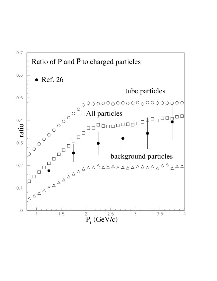
Figure 12: Shows the ratio of protons plus anti-protons to charged particles as a function of $p_{t}$ for particles in our simulated central Au-Au collisions. We also plot the ratio from central Au-Au RHIC data. These experimental results agree well (considering the errors) with the GFTM predictions for all charged particles. The plotted ratio for the background particles coming from HIJING is similar to p-p collisions.

IV The Ridge is formed by the Flux Tubes when a jet trigger is added to the GFTM

In heavy ion collisions at RHIC there has been observed a phenomenon called the ridge which has many different explanations[28-35]. The ridge is a long range charged particle correlation in $\Delta\eta$ (very flat), while the $\Delta\phi$ correlation is approximately jet-like (a narrow Gaussian). There also appears with the ridge a jet-like charged-particle-pair correlation which is symmetric in $\Delta\eta$ and $\Delta\phi$ such that the peak of the jet-like correlation is at $\Delta\eta$ = 0 and $\Delta\phi$ = 0. The $\Delta\phi$ correlation of the jet and the ridge are approximately the same and smoothly blend into each other. The ridge correlation is generated when one triggers on an intermediate $p_{t}$ range charged particle and then forms pairs between that trigger particle and each of all other intermediate charged particles with a smaller $p_{t}$ down to some lower limit.

IV.1 STAR experiment measurement of the ridge

Triggered angular correlation data showing the ridge was presented at Quark Matter 2006Putschke . Figure 14 shows the experimental $\Delta\phi$ vs. $\Delta\eta$ CI correlation for the 0-10% central Au-Au collisions at $\sqrt{s_{NN}}=$ 200 GeV requiring one trigger particle $p_{t}$ between 3.0 and 4.0 GeV/c and an associated particle $p_{t}$ above 2.0 GeV/c. The yield is corrected for the finite $\Delta\eta$ pair acceptance.

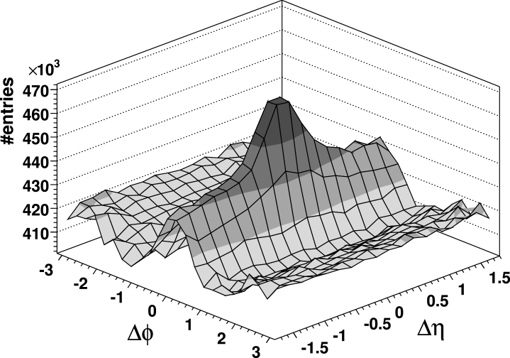
Figure 13: Raw $\Delta\phi$ vs. $\Delta\eta$ CI preliminary correlation dataPutschke for the 0-10% centrality bin for Au-Au collisions at $\sqrt{s_{NN}}=$ 200 GeV requiring one trigger particle $p_{t}$ between 3.0 to 4.0 GeV/c and an associated particle $p_{t}$ above 2.0 GeV/c.

In this paper we will investigate whether the GFTM can account for the ridge once we add a jet trigger to GFTM generatorPBMtoGFTM. However this trigger will also select jets which previously could be neglected because there was such strong quenching[37-39] of jets in central collisions when a jet trigger had not been used. We use HIJINGhijing to determine the number of expected jets. We have already shown that our final state particles come from hadrons at or near the fireball surface. We reduce the number of jets by 80% which corresponds to the estimate that only the parton interactions on or near the surface are not quenched away, and thus at kinetic freezeout fragment into hadrons which enter the detector. This 80% reduction is consistent with single $\pi^{0}$ suppression observed in Ref.quench3 . We find for the reduced HIJING jets that 4% of the Au-Au central events (0-5%) centrality at $\sqrt{s_{NN}}=$ 200 have a charged particle with a $p_{t}$ between 3.0 and 4.0 GeV/c with at least one other charged particle with its $p_{t}$ greater than 2.0 GeV/c coming from the same jet. With the addition of the quenched jets to the generator, we then form two-charged-particle correlations between one-charged-particle with a $p_{t}$ between 3.0 to 4.0 GeV/c and another charged-particle whose $p_{t}$ is greater than 2.0 GeV/c. The results of these correlations are shown in Figure 15.

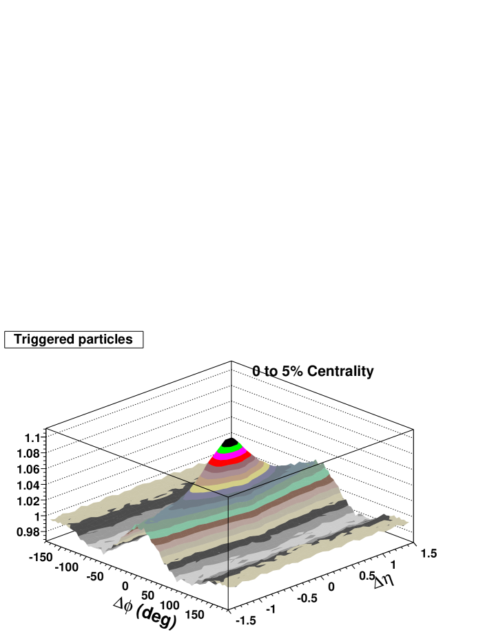
Figure 14: The GFTM generated CI correlation for the 0-5% centrality bin requiring one trigger particle $p_{t}$ above 3.0 GeV/c and less than 4.0 GeV/c and another particle $p_{t}$ above 2.0 GeV/c plotted as a two dimensional $\Delta\phi$ vs. $\Delta\eta$ perspective plot. The trigger requirements on this figure are the same as those on the experimental data in Figure 13.

We can compare the two figures, if we realize that the away-side ridge has around 420,000 pairs in Figure 14 while in Figure 14 the away-side ridge has a correlation of around 0.995. If we multiply the correlation scale of Figure 14 by 422,111 in order to achieve the number of pairs seen in Figure 13, the away-side ridge would be at 420,000 and the peak would be at 465,000. This would make a good agreement between the two figures. We know in our Monte Carlo which particles come from tubes which would be particles form the ridge. The correlation formed by the ridge particles is generated almost entirely by particles emitted by the same tube. Thus we can predict the shape and the yield of the ridge for the above $p_{t}$ trigger selection and lower cut, by plotting only the correlation coming from pairs of particles that are emitted by the same tube (see Figure 15).

In Ref.Putschke it was assumed that the ridge yield was flat across the acceptance while in Figure 14 we see that this is not the case. Therefore our ridge yield is 35% larger than estimated in Ref.Putschke . Finally we can plot the jet yield that we had put into our Monte Carlo. The jet yield is plotted in Figure 16 where we subtracted the tubes and the background particles from Figure 14.

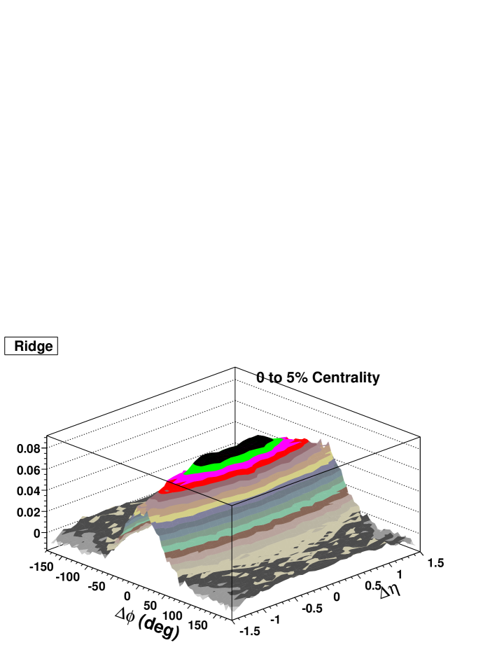
Figure 15: The ridge signal is the piece of the CI correlation for the 0-5% centrality of Figure 15 after removing all other particle pairs except the pairs that come from the same tube. It is plotted as a two dimensional $\Delta\phi$ vs. $\Delta\eta$ perspective plot.

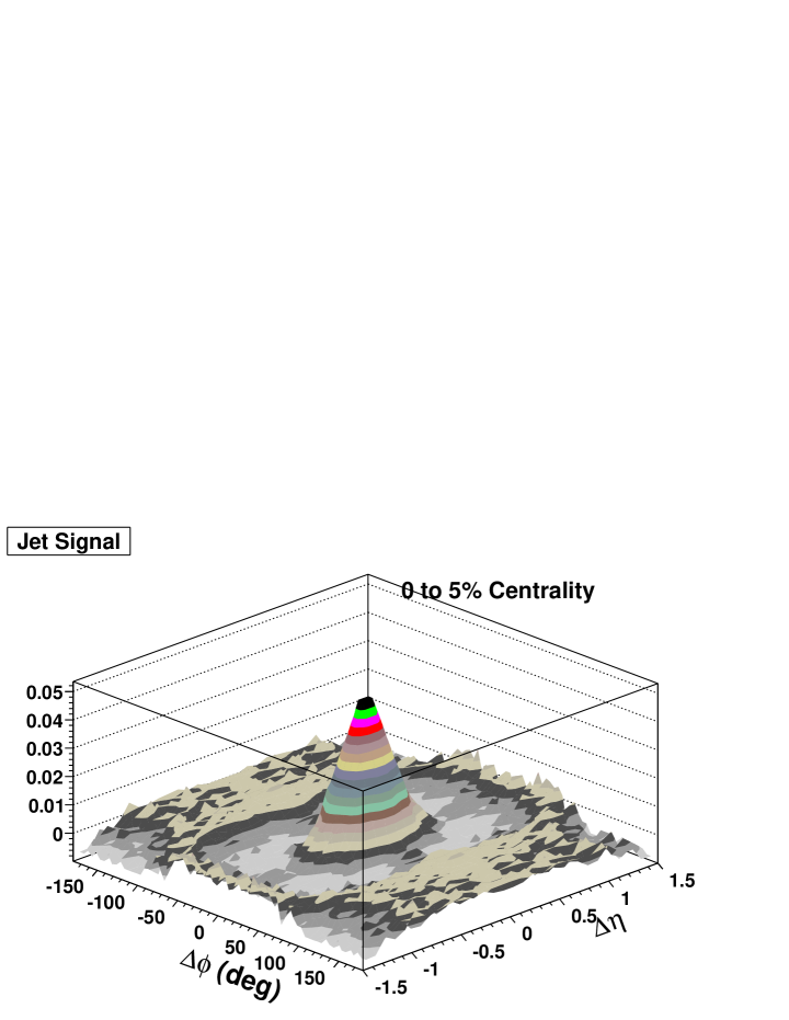
Figure 16: The jet signal is left in the CI correlation after the contributions from the background and all the bubble particles are removed from the 0-5% centrality (with trigger requirements) of Figure 15. It is plotted as a two dimensional $\Delta\phi$ vs. $\Delta\eta$ perspective plot.

IV.2 PHOBOS experiment measurement of the ridge

The PHOBOS detector select triggered charged tracks with $p_{t}$ $>$ 2.5GeV/c within an acceptance of 0 $<$ $\eta^{trig}$ $<$ 1.5. Associated charge particles that escape the beam pipe are detected in a range $|\eta|$ $<$ 3.0. The CI correlation is shown in Figure 17PHOBOS . The near-side structure is more closely examined by integrating over $|\Delta\phi|$ $<$ 1 and is plotted in Figure 18 as a function of $\Delta\eta$. PYTHIA simulation for p-p events is also shown. Bands around the data points represent the uncertainty from flow subtraction. The error on the ZYAM procedure is shown as a gray band at zero. All systematics uncertainties are 90% confidence level.

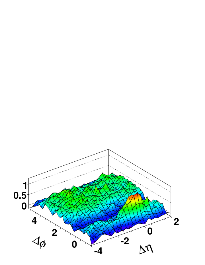
Figure 17: PHOBOS triggered CI correlation from 0-30% central Au-Au collisions. It is plotted as a two dimensional $\Delta\phi$ vs. $\Delta\eta$ perspective plot.

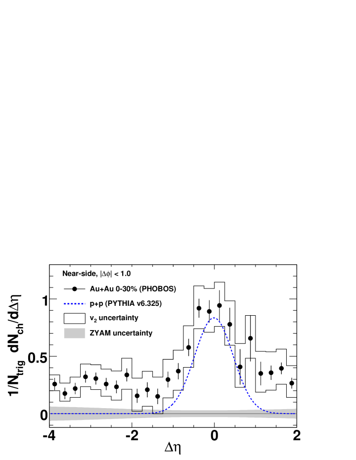
Figure 18: PHOBOS near-side trigger yield integrated over $|\Delta\phi|$ $<$ 1.0 for 0-30% central Au-Au compared to PYTHIA p-p (dashed line) as a function of $\Delta\eta$. Bands around the data points represent the uncertainty from flow subtraction. The error on the ZYAM procedure is shown as a gray band at zero. All systematics uncertainties are 90% confidence level.

We generate using our above GFTM the two-charged-particle correlations between one-charged-particle with a $p_{t}$ between greater than 2.5 GeV/c which has an $|\eta|$ $<$ 0.75 and another charged-particle whose $p_{t}$ is greater than 7 MeV/c in a range $|\eta|$ $<$ 3.0. The results of this correlation is shown in Figure 20. We see that the triggered correlation is vary similar to the PHOBOS results. In order to make a comparison we integrate the near-side structure over $|\Delta\phi|$ $<$ 1 and plot it as a smooth curve in Figure 21 as a function of $\Delta\eta$. We also again plot the PHOBOS points on the same plot. The long range correlation over $\Delta\eta$ produced by the GFTM is possible and does not violate causality, since the glasma flux tubes are generated early in the collision. The radial flow which develops at a later time pushes the surface tubes outward in the same $\phi$ direction because the flow is purely radial. In order to achieve such an effect in minijet fragmentation one would have to have fragmentation moving faster than the speed of light.

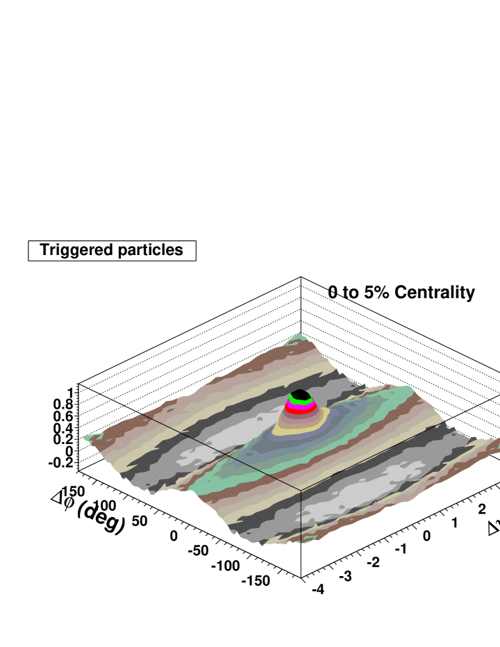
Figure 19: GFTM triggered (see text) CI correlation from 0-5% central Au-Au collisions. It is plotted as a two dimensional $\Delta\phi$ vs. $\Delta\eta$ perspective plot which is the same as Figure 18.

Figure 20: GFTM $\phi$ integrated ($|\Delta\phi|$ $<$ 1) near-side structure compared to PHOBOS near-side structure (see Figure 20).

V The Mach Cone Effect and Three Particle Angular Correlations

It was reported by the PHENIX CollaborationPHENIXCONE that the shape of the away-side $\Delta\phi$ distributions for non-peripheral collisions are not consistent with purely stochastic broadening of the peripheral Au-Au away-side. The broadening and possible change in shape of the away-side jet are suggestive of a mach conerenk . The mach cone effect depended on the trigger particles and the associated particles used in the two particle angular correlations. The mach cone shape is not present if one triggers on 5-10 GeV/c particles and also use hard associated particles greater than 3 GeV/cjiangyong . The away-side broadening in the two-particle depends on the $v_{2}$ subtraction and the method of smearing the away-side dijet component and momentum conservation.

One needs to go beyond two particle correlations in order to learn more. A three particle azimuthal angle correlation should reveal very clear pattern for the mach cone compared to other two particle method. The STAR CollaborationSTARCONE has made such correlation studies and does find a structure some what like a mach cone. However the trigger dependence as seen in Ref.jiangyong and the measurement of the conical emission angle to be independent of the associated particle $p_{t}$ in Ref.STARCONE is not consistent with a mach cone. The similarity of the mach cone and the ridge is very interesting to consider and makes one consider that they are the same effect. In the last section we showed that flux tubes can explain the ridge, thus they should explain the mach cone. One would not expect the minijet model will give a mach cone like correlation.

We saw at the end of Sec. 2 that final state anisotropic flow pattern can be decomposed in a Fourier series ($v_{1}$, $v_{2}$, $v_{3}$, …). When one triggers on a particle coming from a flux tube, the other flux tubes contribute the components of the anisotropic flow pattern. In Figure 22 we show two such tube arrangements. In order to make contact with the data and show the difference between the minijet model and GFTM we will define a trigger particle and a reference particle(s). We choose a $p_{t}$ of greater than 1.1 GeV/c for the trigger and less than this value for the reference. The two particle correlation for this trigger and reference for the minijet model and the GFTM are equal to each other.

Figure 21: Top arrangement has a $v_{3}$ component while the bottom gives a $v_{2}$ component. In most mach cone analyses $v_{2}$ is subtracted.

We define a three particle correlation using the azimuthal angle between a trigger particle 1 and a reference particle 2 ($\Delta\phi_{12}$) and for the third particle the azimuthal angle between a trigger particle 1 and a reference particle 3($\Delta\phi_{13}$). The two particle correlation of the two models are the same and the three particle correlation is nearly the same. In order to obtain the true three particle effect we must remove the two particle correlation from the raw three particle correlation. This removal gives the so-called three particle cumulant. Figure 22 and Figure 23 shows the three particle cumulant for $\Delta\phi_{12}$ vs. $\Delta\phi_{13}$ for the minijet model and the GFTM.

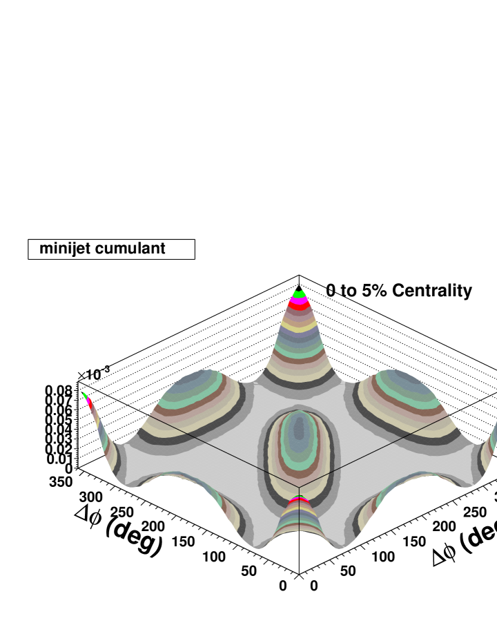
Figure 22: The minijet generated three particle cumulant for the 0-5% centrality bin requiring one trigger particle $p_{t}$ above 1.1 GeV/c and other reference particles $p_{t}$ below 1.1 GeV/c plotted as a two dimensional combinations of trigger particle 1 paired with two reference particles 2 and 3 creating $\Delta\phi_{12}$ vs. $\Delta\phi_{13}$ perspective plot.

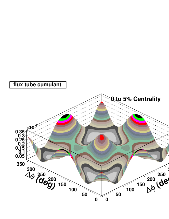
Figure 23: The GFTM generated three particle cumulant for the 0-5% centrality bin requiring one trigger particle $p_{t}$ above 1.1 GeV/c and other reference particles $p_{t}$ below 1.1 GeV/c plotted as a two dimensional combinations of trigger particle 1 paired with two reference particles 2 and 3 creating $\Delta\phi_{12}$ vs. $\Delta\phi_{13}$ perspective plot.

The minijet model Figure 22 shows only diagonal away-side response coming from the underlying dijet nature of the minijets. The GFTM Figure 23 also shows the diagonal away-side response of momentum conservation, however $v_{3}$ configurations of Figure 21 gives an off-diagonal island at $\Delta\phi_{12}$ $\sim$ $130^{\circ}$, $\Delta\phi_{13}$ $\sim$ $230^{\circ}$ or vice versa.

Let us look at the reported STAR dataUlery in order to address this off-diagonal effect. In Figure 24 we show the raw three particle results from STAR where (a) is the raw two particle correlation (points). They also show in (a) the background formed from mixed events with flow modulation added-in (solid). The background subtracted two particle correlation is shown as an inset in (a) where the double hump mach cone effect is clear. In Figure 24(b) the STAR raw three particle correlation is shown which required one trigger particle 3.0 $<$ $p_{t}$ $<$ 4.0 GeV/c and other reference particles 2 and 3 with 1.0 $<$ $p_{t}$ $<$ 2.0 GeV/c. An off-diagonal island does appear at $\Delta\phi_{12}$ $\sim$ 2.3, $\Delta\phi_{13}$ $\sim$ 4.0 radians or vice versa. This is the same values as the island which occurs in the GFTM and is the off-diagonal excess that is claimed to be the mach cone. Like the ridge effect the mach cone seems to be the left overs of the initial state flux tube arrangements related to the fluctuations in the third harmonic. Higher order harmonic fluctuations become less likely to survive to the final state.

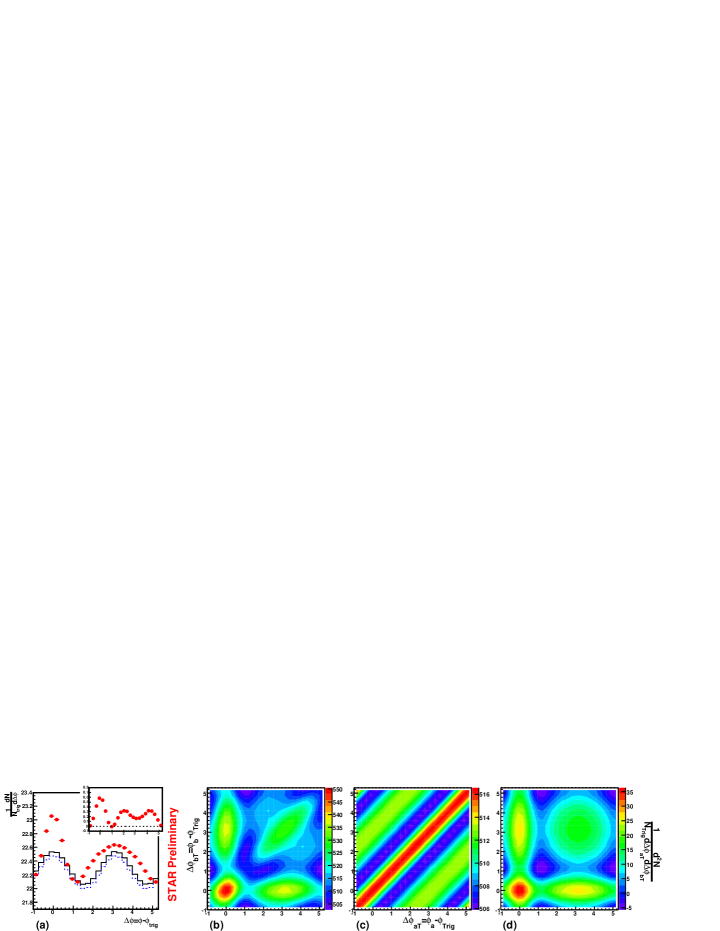
Figure 24: (a) STAR data raw two particle correlation points, background from mixed events with flow modulation added-in (solid) along with the background subtracted two particle correlation (inset). (b) Raw three particle correlation from STAR requiring one trigger particle 3.0 $<$ $p_{t}$ $<$ 4.0 GeV/c and other reference particles 2 and 3 with 1.0 $<$ $p_{t}$ $<$ 2.0 GeV/c creating a two dimensional perspective plot $\Delta\phi_{12}$ vs. $\Delta\phi_{13}$.

VI Summary and Discussion

In this article we have made a comparison between two very different models for central Au-Au collisions. Both models are successful at describing the the spectrum of particles produced and the two particle angular correlations observed in ultrarelativistic heavy ion collisions. The first model is a minijet model which assumes that around $\sim$50 minijets are produced in back-to-back pairs and has an altered fragmentation function from that of vacuum fragmentation. It also assumes that the fragments are transparent and escape the collision zone and are then detected. The second model is a glasma flux tube model which leads to longitudinal color electric and magnetic fields confined in flux tubes on the surface of a radial expanding fireball driven by interacting flux tubes near the center of the fireball through plasma instabilities. This internal fireball becomes an opaque hydro fluid which pushes the surface flux tubes outward. Around $\sim$12 surface flux tubes remain and fragment with $\sim$1/2 the produced particles escaping the collision zone and are detected.

We expand our comparison to other phenomenon of the central collisions. We considered in Sec. 3 baryon and anti-baryon formation in both models. There was no a priori reason for the excess in the minijet model, while in the glasma flux tube model(GFTM) recombination of quarks into di-quarks and anti-quark into anti-di-quarks leads to a natural excess of baryon and anti-baryon formation in this model.

The formation of the ridge phenomena is discussed in Sec. 4. In order to achieve a long range correlation effect in minijet fragmentation one would have to have fragmentation moving faster than the speed of light. The GFTM however can have a long range correlation over $\Delta\eta$ since the glasma flux tubes are generated early in the collision. The radial flow which develops at a later time pushes the surface tubes outward in the same $\phi$ direction because the flow is purely radial. Thus a long range $\Delta\eta$ last to the final state of the collision. A very good comparison was achieved between data and GFTM.

Sec. 5 treats the so-called mach cone effect by analyzing three particle angular correlations in the two models. The minijet model and the GFTM have the same two particle angular correlations but when the three particle azimuthal angular correlations are compared the two models differ. The minijet model shows only diagonal away-side response coming from the underlying dijet nature of the minijets, while GFTM also shows a diagonal away-side response it also shows an off-diagonal island. Like the ridge effect the mach cone seems to be left over from the initial state flux tube arrangements related to the fluctuations in the third harmonic($v_{3}$). This off-diagonal island excess is seen in the data and is claimed to be the mach cone.

Relativistic Heavy Ion Collider (RHIC) collisions are conventionally described in terms of two major themes: hydrodynamic evolution of a thermal bulk medium and energy loss of energetic partons in that medium through gluon bremsstrahlung. The minijet model is not consistent with is standard view. The glasma flux tube model generates a fireball which becomes an opaque hydro fluid that is consistent with conventional ideas. Even though both models can obtain the same spectrum of particles and the same two particle angular correlations, it is only the GFTM that can tie all together.

VII Acknowledgments

This research was supported by the U.S. Department of Energy under Contract No. DE-AC02-98CH10886. The author thank Sam Lindenbaum and William Love for valuable discussion and Bill for assistance in production of figures. It is sad that both are now gone.

References

- (1) T. Trainor, Phys. Rev. C 80 (2009) 044901.
- (2) A. Dumitru, F. Gelis, L. McLerran and R. Venugopalan, Nucl. Phys. A 810 (2008) 91.
- (3) J. Adams et al., Phys. Rev. C 73 (2006) 064907.
- (4) M. Daugherity, J. Phys.G G35 (2008) 104090.
- (5) Q.J. Liu et al., Phys. Lett. B632 (2006) 197.
- (6) J. Adams et al., J.Phys.G G34 (2007) 451.
- (7) J. Adams et al., J Phys.G G32 (2006) L37.
- (8) T. Trainor, Int. J. Mod. Phys. E 17 (2008) 1499.
- (9) J. Adams et al., Phys. Rev. D 74 (2006) 032006.
- (10) D. Kharzeev and M. Nardi, Phys. Lett. B507 (2001) 121.
- (11) T. Trainor and D. Kettler, Phys. Rev. C 83 (2011) 034903.
- (12) L. McLerran and R. Venugopalan, Phys. Rev. D 49 (1994) 2233; Phys. Rev. D 49 (1994) 3352; Phys. Rev. D 50 (1994) 2225.
- (13) T. Lappi and L. McLerran, Nucl. Phys. A 772 (2006) 200.
- (14) F. Gelis and R. Venugopalan, Acta Phys. Polon. B 37 (2006) 3253.
- (15) D. Kharzeev, A. Krasnitz and R. Venugopalan, Phys. Lett. B 545 (2002) 298.
- (16) P. Romatschke and R. Venugopalan, Phys. Rev. D 74 (2006) 045011.
- (17) S. Gavin, L. McLerran and G. Moschelli, Phys. Rev. C 79 (2009) 051902.
- (18) S.J. Lindenbaum, R.S. Longacre, Eur. Phys. J. C. 49 (2007)767.
- (19) S.J. Lindenbaum, R.S. Longacre, arXiv:0809.2286(Nucl-th).
- (20) T. Sjostrand, M. van Zijil, Phys. Rev. D 36 (1987) 2019.
- (21) J. Adams et al., Phys. Rev. C 71 (2005) 044906, S.S. Adler et al., Phys. Rev. Lett. 93 (2004) 152302.
- (22) J. Adams et al., Phys. Rev. C 75, 034901 (2007).
- (23) S.J. Lindenbaum and R.S. Longacre, Phys. Rev. C 78 (2008) 054904.
- (24) B.I. Abelev et al., arXiv:0806.0513[nucl-ex].
- (25) B. Alver and G. Roland, Phys. Rev. C 81 (2010) 054905.
- (26) S.S. Adler et al., Phys. Rev. Lett. 91 (2003) 172301.
- (27) X.N. Wang and M. Gyulassy, Phys. Rev. D 44 (1991) 3501.
- (28) N. Armesto, C. Salgado, U.A. Wiedemann, Phys. Rev. Lett. 93 (2004) 242301.
- (29) P. Romatschke, Phys. Rev. C 75 (2007) 014901.
- (30) E. Shuryak, Phys. Rev. C 76 (2007) 047901.
- (31) A. Dumitru, Y. Nara, B. Schenke, M. Strickland, J.Phys.G G35 (2008) 104083.
- (32) V.S. Pantuev, arXiv:0710.1882[hep-ph].
- (33) R. Mizukawa, T. Hirano, M. Isse, Y. Nara, A. Ohnishi, J.Phys.G G35 (2008) 104083.
- (34) C.Y. Wong, Phys. Rev. C 78 (2008) 064905.
- (35) R.C. Hwa, arXiv:0708.1508[nucl-th].
- (36) J. Putschke, Nucl. Phys. A 783 (2007) 507c.
- (37) C. Adler et al., Phys. Rev. Lett. 88 (2002) 022301.
- (38) J. Adams et al., Phys. Rev. Lett. 91 (2003) 172302.
- (39) A. Adare et al., Phys. Rev. Lett. 101 (2008) 232301.
- (40) B. Alver et al., Phys. Rev. Lett. 104 (2010) 062301.
- (41) S.S. Adler et al., Phys. Rev. Lett. 97 (2006) 052301.
- (42) T. Renk and J. Ruppert, Phys. Rev. C 73 (2006) 11901.
- (43) J. Jia PHENIX, AIP Conf.Proc. 828 (2006) 219.
- (44) B.I. Abelev et al., Phys Rev. Lett. 102 (2009) 052302.
- (45) J.G. Ulery STAR, Int. J. Mod. Phys. E16 (2007) 3123.