On the emergence of very long time fluctuations and $1/f$ noise in ideal flows

Abstract

This study shows the connection between three previously observed but seemingly unrelated phenomena in hydrodynamic (HD) and magnetohydrodynamic (MHD) turbulent flows, involving the emergence of fluctuations occurring on very long time scales: the low-frequency $1/f$ noise in the power frequency spectrum, the delayed ergodicity of complex valued amplitude fluctuations in wavenumber space, and the spontaneous flippings or reversals of large scale fields. Direct numerical simulations of ideal MHD and HD are employed in three space dimensions, at low resolution, for long periods of time, and with high accuracy to study several cases: Different geometries, presence of rotation and/or a uniform magnetic field, and different values of the associated conserved global quantities. It is conjectured that the origin of all these long-time phenomena is rooted in the interaction of the longest wavelength fluctuations available to the system with fluctuations at much smaller scales. The strength of this non-local interaction is controlled either by the existence of conserved global quantities with a back-transfer in Fourier space, or by the presence of a slow manifold in the dynamics.

I Introduction

A characteristic of turbulence is the dynamical involvement of fluctuations over a broad range of length scales. At the largest scales the general expectation is that of non-universal behavior and influence by boundary conditions and/or driving. At intermediate scales, statistical behavior can be obtained, and at the smallest scales, behavior is determined by some dissipation mechanism. Associated with these length scales, there are corresponding ranges of time scales. The characteristic nonlinear time scale, assuming local interactions in scale, is obtained dimensionally as the ratio $l/u_{l}$, where $l$ is a length and $u_{l}$ is the corresponding typical velocity at $l$. Suppose we choose a particular length $L$ and its associated time scale $L/u_{L}$ as the unit of time measurement. Frequently $L$ will be the largest length scale in the system, or perhaps the size of the energy-containing eddies. In these units the range of locally computed time scales $l/u_{l}$ will typically extend from unity (or times of order one) to smaller time scales at the smaller length scales. However, there are some situations in which there is an emergence of much longer time scales, which cannot be associated with this kind of an estimate that is local in scale. Some of these issues have previously been identified in numerical simulations DmitrukMatthaeus07 , for example in the case of a driven-dissipative three-dimensional (3D) magnetohydrodynamic (MHD) system in presence of a strong background magnetic field, and in two-dimensional (2D) hydrodynamic (HD) and MHD driven-dissipative systems. In those three cases, the presence of long time fluctuations is connected with the appearance of a $1/f$ noise type frequency power spectrum at very low frequencies $<<u_{L}/L$. In many situations a $1/f$ noise spectrum arises from the existence of multiple correlation times in the system (see vanderZiel50 ). Such $1/f$ spectra associated with long time scale fluctuations have been observed in a wide range of situations Machlup ; MontrollShlesinger82 but the presence of $1/f$ noise in turbulent flows was reported only recently DmitrukMatthaeus07 . Dynamo simulations of the generation of magnetic fields also exhibit $1/f$ spectra PontyEA04 . Low frequency dynamics have also been reported in laboratory experiments of HD and MHD flows delaTorre07 ; Monchaux09 . Closely related are observations in the solar wind of $1/f$ behavior in the spacecraft frame magnetic and density spectra at low frequencies MatthaeusGoldstein86 ; MatthaeusEA07 . However in the solar wind case the $1/f$ signal appears to trace back to the corona or even to the photosphere BemporadEA08 . It is therefore a consequence of long time scale variability of the solar wind sources, rather than a property that emerges due to solar wind dynamics itself.

It is conjectured in DmitrukMatthaeus07 that the long time fluctuations in the turbulent MHD flows arise from the non-local couplings between the longest length scale in the system (the $k=1$ mode in Fourier space) with the smaller scales, from the inertial to the dissipation range ($k\gg 1$). Such non-local interactions are known to be stronger for MHD than for HD flows Alexakis05 ; Mininni11 . It remains however an open issue as to whether the existence of dissipation, the effects of the driving, or the particular choice of boundaries, are influential in determining the character or presence of the $1/f$ noise that is generated. The present study attempts to show that the presence of a $1/f$ noise spectral regime is specifically with the structure of the equations and the non-linear couplings. We accomplish this by employing a series of numerical simulations of ideal flows in a variety of situations. We emphasize that these simulations are neither dissipative, nor driven. Furthermore, the $1/f$ regime will be characterized by showing its existence (or absence), and its range of frequencies, for several different kinds of ideal flows and geometries. We will argue that a key feature in each system is the existence of either ideal global invariants, or quasi-invariants (to be defined below), which provide constraints on behavior of a small number of important degrees of freedom in the system.

We will further argue below that a related issue concerning ideal flows is the phenomenon of delayed ergodicity ServidioEA08 , also identified as broken ergodicity Shebalin89 ; Shebalin10 . In this phenomenon, the ideal flow is described as a statistical mechanical system composed of Fourier modes (degrees of freedom). Some of these Fourier modes (those corresponding to the largest length scale in the system) appear to spend long periods of time in restricted regions of phase space (i.e., in some interpretations, thus breaking the ergodicity assumption in statistical mechanical systems). As it will be clear from the present study, this effect is essentially the same as that which produces the $1/f$ spectra.

Additionally, we make a further connection with another phenomenon observed on long times scales – the spontaneous flipping or reversal of some large scale fields. A prominent example is the reversal of magnetic field or its magnetic dipole in MHD systems, an effect well known in the context of geomagnetic studies GlatzmaierRoberts95 ; Benzi05 ; Sorriso-ValvoEA07 .

The organization of the paper is as follows. In section II the model equations, the standard ideal equations of HD and MHD flows, are introduced, and the numerical method to solve them is described. In section III the results are presented, divided into subsections for different kinds of systems. In section IV a discussion is developed, followed by the conclusions and summary in section V.

II Model equations

In this paper we consider several systems of equations, including HD flows with and without rotation, and MHD flows with and without externally imposed magnetic fields. We also consider an approximation of the MHD equations in the limit of strong imposed magnetic fields, the so-called reduced MHD (RMHD) equations. All systems are three-dimensional, and the flows are incompressible and ideal (zero dissipation coefficients).

In the most general case, the incompressible HD and MHD equations can be written in dimensionless form as

$$\frac{\partial{\bf u}}{\partial t}+{\bf\omega}\times{\bf u}+2{\bf\Omega}\times{\bf u}=-\frac{1}{\rho}\nabla{\cal P}+{\bf j}\times{\bf B},$$ (1)

$$\frac{\partial{\bf B}}{\partial t}=\nabla\times({\bf u}\times{\bf B}),$$ (2)

where ${\bf B}$ is the magnetic field, ${\bf u}$ the velocity field, ${\bf j}=\nabla\times{\bf B}$ the current density, ${\bf\omega}=\nabla\times{\bf u}$ the vorticity, and ${\cal P}$ the pressure. A term considering rigid rotation with angular velocity $\Omega$ can be included in the velocity equation. This term corresponds to the Coriolis force, with the centrifugal force absorbed into the total pressure term. The pressure can be obtained taking the divergence of the velocity equation, using the incompressibility condition $\nabla\cdot{\bf u}=0$, and solving the resulting Poisson equation. The solenoidal ($\nabla\cdot{\bf B}=0$) magnetic field includes a uniform part ${\bf B_{0}}$ and a fluctuating part ${\bf b}$, so that ${\bf B}={\bf b}+{\bf B_{0}}$.

With ${\bf B_{0}}=0$, these equations reduce to the MHD equations without an external field. When ${\bf B}\equiv 0$, the equations are the ideal incompressible three-dimensional hydrodynamic equations, that is, the Euler equations, which we also consider as a case study. Finally, when ${\bf\Omega}\neq 0$ any of these systems is written in a rotating frame, while ${\bf\Omega}=0$ corresponds to the non-rotating case.

The RMHD equations can be derived from Eqs. (1) and (2) for ${\bf\Omega}=0$ and in the limit of strong ${\bf B_{0}}=B_{0}\hat{\bf z}$, assuming low frequencies and weak spatial gradients along the direction of the background magnetic field Strauss76 ; Montgomery82 . The equations involve potentials $a(x,y,z,t)$ and $\psi(x,y,z,t)$ such that in rectangular $(x,y,z)$ coordinates one has ${\bf b}=\nabla_{\perp}\times\hat{\bf z}a$ and ${\bf u}=\nabla_{\perp}\times\hat{\bf z}\psi$, where $\nabla_{\perp}=(\partial_{x},\partial_{y},0)$. To get slow dynamics as ${\bf B}_{0}\sim 1/\epsilon\to\infty$, for small $\epsilon$, one is forced to an ordering such that $\partial_{z}=O(\epsilon)$. In this sense the RMHD equations are “quasi-two dimensional” in $x$ and $y$. The dynamical equations become simply those of the potentials,

$$\frac{\partial\omega}{\partial t}+{\bf u}\cdot\nabla_{\perp}\omega= {\bf b}\cdot\nabla_{\perp}j+B_{0}\frac{\partial j}{\partial z}+\mu\nabla^{2}\omega$$

$$\frac{\partial a}{\partial t}+{\bf u}\cdot\nabla_{\perp}a= B_{0}\frac{\partial\psi}{\partial z}+\mu\nabla^{2}a$$ (3)

where the electric current density is $j=-\nabla^{2}a$ and the vorticity is $\omega=-\nabla^{2}\psi$.

In the subsequent section we will describe numerical results obtained with two different type of codes, which we now describe briefly. The parameters of all runs discussed below are given in Table I for reference.

For one set of numerical simulations, we assume periodic boundary conditions in a cubic box, of side $2\pi L_{0}$ in each cartesian direction, with $L_{0}$ the arbitrary unit of length. Fields can then be decomposed in Fourier modes

$${\bf u}=\sum_{\bf k}{\bf u}_{\bf k}{\rm e}^{i~{}{\bf k}\cdot{\bf r}}~{},~{}{\bf b}=\sum_{\bf k}{\bf b}_{\bf k}{\rm e}^{i~{}{\bf k}\cdot{\bf r}}~{},$$ (4)

where ${\bf u}_{\bf k}$, ${\bf b}_{\bf k}$ are the Fourier coefficients of the expansion, and ${\bf k}$ is the wavevector, having integer components in the dimensionless case.

We employ a pseudospectral code to accurately numerically solve these equations. With the pseudospectral method (using full de-aliasing with the 2/3 rule) any quadratic invariant (like the total energy) is exactly maintained, except for machine round-off errors and time integration discretization errors. Time integration here is done with a second-order Runge-Kutta method, with a very small time step $dt$, to control the discretization error over the long simulations we carry out. Typically we use $dt\sim 5\times 10^{-4}$ which is much less than the global large scale turnover time $L_{0}/u$, where $u$ is the root mean square (rms) velocity. As an example, in an integration of 1000 unit times duration, for initial primitive fluctuation fields $\bf u$ and $\bf b$ with rms values of 1, these values remain equal to unity with an error less than $5\times 10^{-6}$ at the end of the integration. In dissipative MHD the energy $E$ balance equation satisfies

$$\frac{dE}{dt}=-2\nu(<j^{2}>+<\omega^{2}>)$$ (5)

The decay in energy due to time discretization errors can be interpreted as numerical dissipation and for the example mentioned, using a time averaged value for $<j^{2}>+<w^{2}>\sim 10$, the numerical viscosity is estimated as $\nu\sim 10^{-10}$.

In a second set of numerical simulations, we consider spherical geometry: the HD or MHD equations are solved inside a sphere of unit dimensionless radius, with vanishing velocity and magnetic field at the sphere boundary. For this geometry, a fully spectral Galerkin code is used, based on a Chandrasekar-Kendall (C-K) decomposition of the fields. The C-K functions Chandrasekhar57 ; Montgomery78 are

$${\bf J}_{i}=\lambda\nabla\times{\bf r}\psi_{i}+\nabla\times\left(\nabla\times{\bf r}\psi_{i}\right),$$ (6)

where we work with a set of spherical orthonormal unit vectors $(\hat{r},\hat{\theta},\hat{\phi})$, and the scalar function $\psi_{i}$ is a solution of the Helmholtz equation, $(\nabla^{2}+\lambda^{2})\psi_{i}=0$. The explicit form of $\psi_{i}$ is

$$\psi_{i}(r,\theta,\phi)=C_{ql}\,j_{l}(|\lambda_{ql}|r)Y_{lm}(\theta,\phi),$$ (7)

where $j_{l}(|\lambda_{ql}|r)$ is the order-$l$ spherical Bessel function of the first kind, $\{\lambda_{ql}\}$ are the roots of $j_{l}$ indexed by $q$ (so that the function vanishes at $r=1$), and $Y_{lm}(\theta,\phi)$ is a spherical harmonic in the polar angle $\theta$ and the azimuthal angle $\phi$. The sub-index $i$ is a shorthand notation for the three indices $(q,l,m)$; $q=1,2,3,\dots$ corresponds to the positive values of $\lambda$, and $q=-1,-2,-3,\dots$ indexes the negative values; finally $l=1,2,3,\dots$, and $-l\leq m\leq l$. The C-K functions satisfy

$$\nabla\times{\bf J}_{i}=\lambda_{i}{\bf J}_{i}\ .$$ (8)

With the proper normalization constants, they are an orthonormal set that has been shown to be complete Cantarella00 . The values of $|\lambda_{i}|$ play a role similar to the wavenumber $k$ in the Fourier expansion. Note that boundary conditions, as well as the Galerkin method to solve the equations inside the sphere using this base, were chosen to ensure conservation of all quadratic invariants of the systems, crucial for our present study of ideal flows for long times. More details about the technique to numerically solve the HD and MHD equations in this spherical geometry can be found in Mininni06 ; Mininni07 .

III Results

III.1 Three-dimensional MHD in a box and in the sphere

For three-dimensional incompressible ideal MHD with no mean magnetic field, there are three quadratic invariants: the total (kinetic plus magnetic) energy per unit mass

$$E=\frac{1}{2}\langle|{\bf u}|^{2}+|{\bf b}|^{2}\rangle\ =\ E_{u}+E_{b},$$ (9)

(with $\langle\dots\rangle$ denoting a spatial average), the cross helicity

$$H_{c}=\langle{\bf u}\cdot{\bf b}\rangle\,,$$ (10)

and the magnetic helicity

$$H_{m}=\langle{\bf a}\cdot{\bf b}\rangle\,$$ (11)

, where ${\bf a}$ is the vector potential such that $\nabla\times{\bf a}={\bf b}$. The robustness of the Gibbs equilibrium ensemble predictions for this system is well established Lee52 ; Kraichnan65 ; Shebalin83 ; FrischEA75 ; StriblingMatthaeus90 . The expectation value of spectra are readily obtained in the Gibbs ensemble using Lagrange multipliers associated with each conserved quantity. These expectations are well verified with numerical simulations FrischEA75 ; StriblingMatthaeus90 . Usually the Gibbs ensemble has been viewed as a predictor of the direction of spectral transfer, although more recently it has also been found that the ideal Gibbs-Galerkin system shares additional characteristics with the dissipative turbulent system at short and intermediate time scales and length scales. One of the characteristics found is that even in the ideal truncated case, cascades develop during transients (brachet ; KrstulovicEA09 ; WanEA09 ; giorgio ). For long times the system goes to solutions with zero flux but any perturbation of the system away from the zero flux solutions (e.g., by thermal fluctuations) is corrected by transient non-zero fluxes associated with the non-linear interactions (Mininni11DMP ).

For wavenumber $k>>1$ (the wavenumber $k$ in the following discussion should be considered equivalent to $|\lambda_{i}|$ for the spherical case), the Gibbs ensemble predicts in three-dimensions an omnidirectional spectrum going like $k^{2}$. Attaining this equilibrium prediction is frequently called “thermalization” of the large wavenumber modes, as this corresponds to equipartition of energy among all individual modes, i.e., a flat modal spectrum. At the fundamental modes $k=1$ (the largest possible wavelength modes in a finite size system), condensation is predicted, according to the established value of $H_{m}$. When $H_{m}\neq 0$, condensation at the $k=1$ mode occurs, and this has been the base for prediction FrischEA75 of an inverse cascade of magnetic helicity in dissipative MHD (i.e., when dissipation and forcing is added to the ideal MHD equations).

Furthermore, when both $H_{m}\neq 0$ and $H_{c}\neq 0$, the condensation of magnetic helicity induces a partial condensation of the cross helicity StriblingMatthaeus90 . For such cases the largest scales are expected to contain signatures both of magnetic helicity (helical ${\bf b}$) and of Alfvénic correlation (${\bf u}\propto{\bf b}$).

We note here that the ideal model can be viewed as a dynamical model of the nonlinearities that drive turbulence. It is a simplified model because it becomes Gaussian, and also it lacks a preferred average direction of spectral transfer. But it is worth remembering that in “real turbulence”, with dissipation, there are large numbers of couplings that take energy to higher $k$, and also large numbers of couplings that take energy to lower $k$. These two types of couplings are almost in balance. However, transfer to higher $k$ dominates slightly – this is just what the direct cascade is (an inverse cascade would be the case where the transfer to lower $k$ dominates slightly). This has been observed in numerical simulations, as well as in laboratory experiments. In this regard, the ideal model is not “real turbulence” but it shares some of its properties (brachet ).

An assumption for the equilibrium ensemble predictions is the property of ergodicity. The required property is that, in a long period of time, the system, defined by the set of real and imaginary parts of its Fourier coefficients (i.e., the dynamical degrees of freedom of the ideal MHD system) will visit all accessible regions in complex phase space. A point in phase space is “accessible” if it is permitted by the values of the invariant quantities. This is well verified for $k>1$ modes, which evolve on relatively fast time scales. However, for the longest wavelength $k=1$ modes there is an apparent breaking of ergodicity that has been identified in simulations Shebalin89 ; Shebalin10 . There is however evidence that ergodicity is restored at very long times ServidioEA08 . As a result, the $k=1$ modes seem to wander for very long periods of time in restricted regions of phase space, until at some point, a possibly sudden “hopping” ServidioEA08 occurs and a new period of wandering occurs in another restricted region of phase space. As has been recently also pointed out Shebalin10 , the time duration of these wandering periods is related to the dimension of the system (i.e., the finite number of modes assumed for the numerical simulation). This is to be expected since the delayed ergodicity is related to condensation, and for any system with the same values of the ideal invariants, the condensation is more complete for systems with larger numbers of degrees of freedom StriblingMatthaeus90 .

We will focus here then on the time behavior of a single $k=1$ mode, and the point we make is that there is a connection between this aperiodic cycle of wandering and hopping behavior, and the $1/f$ power frequency spectrum already observed in dissipative MHD DmitrukMatthaeus07 . The time behavior of the $k=1$ mode can be interpreted as the time behavior of the large scale magnetic field, i.e., it corresponds to the time behavior of the fluctuating magnetic field after a filtering of the smaller scales (with $k>1$) is performed. This connection between $k=1$ and the apparent or observable large scale magnetic field becomes sharper as the condensation becomes more complete. In dissipative MHD, this filtering process occurs naturally through dissipation which damps the small scales. In ideal MHD, however, the thermalization of the small scales, with a spectrum going like $k^{2}$, tends to obscure the time behavior of the $k=1$ mode if a power frequency analysis is applied to the full fluctuating magnetic field. As a result, we shall look at the time behavior of a single $k=1$ mode in this case, in order to properly see the long time fluctuations that develop. In what follows, we thus present a series of results for the time behavior and the frequency spectrum of the $k=1$ mode for different numerical simulations of ideal MHD, with first a fixed system size (fixed $N$, with $N^{3}$ = total number of modes) and varying the magnetic helicity, and secondly by varying the number of modes $N^{3}$ but with approximately fixed magnetic helicity. Our working hypothesis is that these scalings can be understood in terms of scalings within the Gibbs ensemble StriblingMatthaeus90 : For fixed $H_{m}/E$, increasing $N$ intensifies the condensation until all $H_{m}$ asymptotically resides in $k=1$. For fixed $N$, increasing $H_{m}/E$ increases condensation until as this ratio approaches its maximum value, all excitations condense to $k=1$.

III.1.1 Periodic box

We begin by considering the behavior in time of a large scale mode in a sequence of three incompressible ideal 3D MHD simulations with increasing $|H_{m}|$. These are further described in Table I, and have $H_{m}=-0.008$, $0.129$, and $-0.395$, a fixed simulation size of $N^{3}=16^{3}$, and fixed total energy equal to $1$. The fluctuations are initially equipartitioned $E_{u}=E_{b}$, and concentrated in a range of wavenumbers $1<k<4$. In particular Figure (1) illustrates the temporal behavior of the $k=1$ modes, choosing the real part of $b_{z}({\bf k}=1,0,0)$ as an indicator of the behavior of the large-scale modes. Indeed, the same behavior is obtained for other components, $b_{x}$, $b_{y}$, or for other directions in ${\bf k}$, except of course for directions for which ${\bf k}$ is parallel to the field component, which are identically zero due to the $\nabla\cdot{\bf b}=0$ condition. The different panels in Figure (1) correspond to increasing values of $|H_{m}|$. It is apparent that as the magnitude of magnetic helicity is increased, long period fluctuations (as long as $1000$ unit times) begin to appear. Such fluctuations are not observed in the time series of modes with larger wavenumber (i.e., smaller spatial scales), and are characteristic of the largest scale Fourier modes in the system. Note that the value of the magnetic field fluctuation amplitude increases with $H_{m}$, consistent with the condensation phenomenon.

Qualitatively, it would be reasonable to say that the low helicity case in Figure (1) (top) is more “stationary”, as the fluctuations in that case approach a zero mean within say 100 time units or less. On the other hand the two higher helicity cases exhibit coherent fluctuations at a scale of hundreds, or even thousands, of time units. The suggestion is that low frequency oscillations are becoming more dominant with higher helicity. Indeed, there is clear evidence of this in the frequency spectra, shown in Figure (2) for each of the three time series given in Figure (1). The increasing power in the low frequency part, and the emergence of a $\sim 1/f$ power law at the very low frequencies $<<1$ , are associated with increasing $|H_{m}|$. We note here that often in the literature, $1/f$ is loosely used to refer to any spectrum of the form $f^{-\alpha}$, with $0<\alpha<2$ (i.e. omitting both white noise and Brownian motion).

The important point that we want to stress here is not the exact power law index that fits the spectra (which in fact is dependent on the time duration of the simulations, because when longer time fluctuations appear a more extended run would be needed), but rather the fact that there is no obvious reason for which fluctuations with time scales orders of magnitude longer than the unit time should appear here. The longest time scale based on local time arguments is $T_{L}=L/u_{L}$, which for the largest length scale of $L=2\pi$ (box size) corresponding to $k=1$ and for $u_{L}=1$, is $T_{L}=2\pi$. Frequencies below $f_{L}=1/T_{L}=1/(2\pi)$ should normally have a flat power spectrum (white noise), indicating the existence of a defined correlation time. However as the Figure (2) shows, for the cases where long time fluctuations appear, the spectrum to the left of the $f_{L}=1/(2\pi)$ is far from being flat. This is indicated in the panels of the figure with a vertical line at the frequency $1/(2\pi)$ and a horizontal line at the corresponding value of the power spectrum for that frequency. We identify the difference between the observed power spectrum and a flat power spectrum as the range of $1/f$ spectra in each case (again, using a loose definition for $1/f$).

This range of the $1/f$ spectra is short for the lower values of $H_{m}$, with corresponding time periods ($T\sim 1/f$) of the order of $10$ unit times, and increasing to $T\approx 100-500$ for $H_{m}=0.129$, and as long as $T\approx 500-1000$ for $H_{m}=0.395$.

It is interesting to observe the autocorrelation function for each of the time series in the cases shown, as a complementary way to see the appearance of long time fluctuations. Here the autocorrelation function is defined as

$$C(t)=<b(t_{0})b(t_{0}+t)>$$ (12)

where $b$ represents a cartesian component of a magnetic field mode (for instance the $z$ component of the real part of the magnetic field Fourier mode for $k=(1,0,0)$), with subtracted mean and normalized so that $<b^{2}>=1$, $t_{0}$ is an arbitrary origin in time, $t$ is the time lag and $<...>$ denotes a time average.

This is shown in the panels of Figure (3). The case with smallest $H_{m}$ presents a compact correlation function, localized within about $10$ unit times, whereas the cases with larger $H_{m}$ show a much broader correlation function. A correlation time can be obtained as

$$t_{c}=\int_{0}^{T_{f}}C(t)dt$$ (13)

where $T_{f}$ is the final time of the run, assuming it is a large time.

This quantity is well defined if the correlation function is confined within a finite range of time lags, decaying faster for long times. However, if the correlation function does not decay faster, and in depends on the time duration of the series, then the correlation time is not well defined. In particular, for an exact $1/f$ power spectrum there is no single correlation time that can be defined. The values indicated in the plot for the three $H_{m}$ cases of $t_{c}=14,189,346$ show again that longer time fluctuations (and correlations) appear as $H_{m}$ is increased.

Recalling that condensation in the ideal Gibbs ensemble intensifies as the number of degrees of freedom ($\sim N^{3}$) increases, we now explore whether the emergence of long time scale coherent fluctuations and the associated $1/f$ spectra behave the same way. The next series of plots in Figure (4) show the time behavior of a magnetic field component of a single mode ${\bf k}=(1,0,0)$ varying the size of the simulation of 3D MHD, for $N^{3}=16^{3},32^{3}$, and $64^{3}$, and for low values of $H_{m}=0.027$, $0.027$, and $0.015$, respectively. for each $N$. These results show that long time fluctuations appear even for low values of $H_{m}$ when the size of the system is increased. We note that for the $N=64$ case a longer time range is needed to observe fluctuations to average to zero. This is indeed observed in this run when it is extended until $t>10000$ but not shown here for consistency with the shorter time range selected for the rest of the cases in this Figure. Figure (5) shows the corresponding power frequency spectra $P(f)$ for each size $N$. The range of low frequency $1/f$ noise increases from $T\sim 10$ for $N=16$ to $T\sim 2000$ for $N=64$ (compare Figures (2) and (5)).

Furthermore, Figure (6) shows the autocorrelation function and the obtained correlation time $t_{c}$ for each time series for different values of $N$. Also evident in this figure is the appearance of long time fluctuations as $N$ is increased through the broadening of the autocorrelation function.

Figure 1: Time series of a component of the magnetic field for the ${\bf k}=(1,0,0)$ mode in a MHD run with $16^{3}$ modes and with different values of the magnetic helicity: $H_{m}=-0.008$ (top), $0.129$ (middle), and $-0.395$ (bottom).

Figure 2: Power frequency spectra of the time series in Figure (1), with different values of the magnetic helicity $H_{m}=-0.008,0.129$, and $-0.395$. The reference vertical line corresponds to a frequency value $f_{L}=1/(2\pi)$ (see text) and the horizontal line to the value of $P(f_{L})$.

Figure 3: Self-correlation function for the time series of magnetic field in Figure (1), with different values of the magnetic helicity $H_{m}=-0.008,0.129$, and $-0.395$. A correlation time $t_{c}$ (see text) is indicated in each case.

Figure 4: Time series of a component of the magnetic field for $k=(1,0,0)$ mode in the MHD runs with different resolution $N^{3}=16^{3},32^{3}$, and $64^{3}$ and magnetic helicity $H_{m}=0.027,0.027$, and $0.015$.

Figure 5: Power frequency spectra of the time series in Figure (4), with different resolution $N^{3}=16^{3},32^{3}$, and $64^{3}$ and magnetic helicity $H_{m}=0.027,0.027$, and $0.015$. The reference vertical line corresponds to a frequency value $f_{L}=1/(2\pi)$ (see text) and the horizontal line to the value of $P(f_{L})$.

Figure 6: Self-correlation function for the time series of magnetic field in Figure (4), with different resolution $N^{3}=16^{3},32^{3}$, and $64^{3}$ and magnetic helicity $H_{m}=0.027,0.027$, and $0.015$. A correlation time $t_{c}$ (see text) is indicated in each case.

Another view of the long time fluctuations can be obtained from the time evolution of individual Fourier modes in a phase space plot in the complex plane Shebalin89 ; Shebalin10 . For instance, the $b_{z}(1,0,0)$ mode for the $32^{3}$ run in the $H_{m}=0.027$ case is shown in Figure (7). For comparison, the behavior in the complex plane of the $b_{z}(2,0,0)$ mode, with a larger $k$, for the same run is shown in Figure (8). The long time fluctuations of the $b_{z}(1,0,0)$ mode correspond to long periods of time spent in a restricted region in the complex plane, as contrasted by the quick filling of the complex plane allowed region for the $b_{z}(2,0,0)$ case. This phenomenon has been called ServidioEA08 “delayed ergodicity,” because the ergodicity property of the $k=1$ seems to be broken only temporarily, as the mode spends long times in a region of the complex plane thus not filling the entire space. For longer times, the “hopping” of the mode between different regions starts filling the space. As observed here, this corresponds to long time fluctuations of the time series, and to the appearance of the $1/f$ power law in the power frequency spectrum.

As can be seen in the time series plots, the component of the large scale magnetic field shown, which is a dominant contribution to the global magnetic field when condensation is strong, progresses for long periods of time without changing sign, and then experiences a reversal in sign, followed by another long period of time without sign change (see e.g., Figures (1) and (4)). We will come back to this “reversal” phenomenon in spherical runs, but it can already be seen that this is part of the same long time fluctuations phenomenon reported as $1/f$ noise.

Figure 7: Complex phase space trajectory for the ${\bf k}=(1,0,0)$ mode in the MHD $32^{3}$ run, with $H_{m}=0.027$, for different intervals of time.

Figure 8: Complex phase space trajectory for the ${\bf k}=(2,0,0)$ mode in the MHD $32^{3}$ run, with magnetic helicity $H_{m}=0.027$. Notice the noticeably larger wandering in phase space when compared to Figure (7), indicative of clearer ergodicity.

Another interesting diagnostic is shown in Figure (9), where the real and imaginary parts of the complex amplitudes of several field components of the mode ${\bf k}=(1,0,0)$ are shown as a function of time, for the same run ($N^{3}=32^{3}$ and $H_{m}=0.027$). This is a case with long time fluctuations and delayed ergodicity. Apparently, from our analysis the $k=1$ magnetic modes satisfy particular equilibrium configurations, namely the field is quasi force-free. A force-free magnetic field satisfies ${\bf j}\times{\bf b}=0$, that is, the Lorentz force term in the momentum equation is zero. If the velocity field ${\bf u}$ is zero, this means that for an ideal flow (no viscosity or diffusivity) the magnetic field will remain force-free in time, and all non-linear terms will be zero. Force-free states also correspond to maximum allowable values of the magnetic helicity (see Moffattbook ).

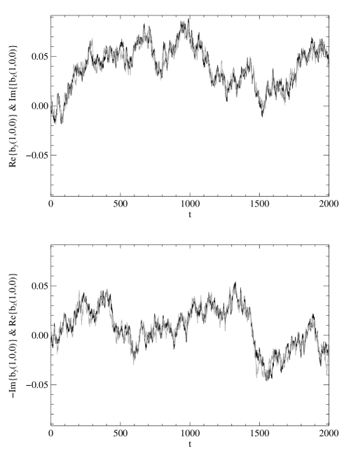
Figure 9: Top: real part of the $b_{y}$ component of the ${\bf k}=(1,0,0)$ mode vs time (black), and imaginary part of $b_{z}$ for the ${\bf k}=(1,0,0)$ mode vs time (light gray) for the MHD $32^{3}$ run with magnetic helicity $H_{m}=0.027$. Bottom: imaginary part of $-b_{y}$ for the ${\bf k}=(1,0,0)$ mode vs time (black), and real part of $b_{z}$ for the ${\bf k}=(1,0,0)$ mode vs time (light gray).

In terms of Fourier modes, if a single ${\bf k}$ mode is in a force-free state, i.e., ${\bf j_{k}}\times{\bf b_{k}}=0$, then, since ${\bf j_{k}}=i{\bf k}\times{\bf b_{k}}$, it must satisfy $i{\bf k}\times{\bf b_{k}}=\lambda{\bf b_{k}}$ which implies that $\lambda^{2}=k^{2}$, that is, $\lambda=\pm k$. For the $k=1$ modes this means $\lambda=\pm 1$ and, since these modes are equal to the Cartesian versors (unit vectors), it also implies some relations between the components of ${\bf b_{k}}$. Taking, for example, ${\bf k}=(1,0,0)$, these relations are $Im(b_{z})=\pm Re(b_{y})$ and $Re(b_{z})=\mp Im(b_{y})$, where the field components are in k-space (notice that for this mode, $b_{x}=0$ because of the divergence-free condition.) This is immediately seen to be the condition for a circularly polarized fluctuation in a k-aligned coordinate system – that is, if we let ${\bf k}=(1,0,0)$ in a right-handed Cartesian system, then the above conditions are equivalent to ${\bf b_{k}}=e^{\phi_{k}}(0,1,\pm i)$ for arbitrary phase $\phi$. The plots in Figure (9) show that the imaginary and real parts of these field components exhibit this correlation – they are very highly correlated in time (light gray and black are used for each corresponding component and are almost indistinguishable). In fact, values of the correlation coefficient $>0.95$ are obtained in each case, corresponding to near maximum helicity.

Similar relations can be found for the ${\bf k}=(0,1,0)$ and ${\bf k}=(0,0,1)$ modes, and strong correlations $>0.95$ are also found for the imaginary and real part of the corresponding field components in time (not shown). This is true for all the previous runs for which long time fluctuations of the $k=1$ modes are observed. However the circular polarization is not found for larger $k$ modes (e.g., for ${\bf k}=(2,0,0)$). This is a very special property of the $k=1$ modes, that they evolve in a quasi force-free state in time. This condition is consistent with the ensemble average predictions of the Gibbsian theory FrischEA75 ; StriblingMatthaeus90 , but is not imposed by it as an exact condition due to allowance for fluctuations about the equilibrium expectation. We will come back to this issue in the discussion section.

III.1.2 Spherical geometry

The next example corresponds to a series of spherical MHD runs. Figure (10) shows three runs with a fixed value of $H_{m}=0.03$, and with three different values of $q_{max}=5,7$, and $8$, corresponding to increasing number of degrees of freedom in the model. Here, $q_{max}$ is the maximum value of the $q$ index corresponding to the radial number in a spherical harmonic expansion [see Eqs. (6)-(7) and text therein]; the maximum values of $l$ and $m$ are also increased accordingly. In this particular geometry, the maximum possible value of helicity for a flow with unit energy is $\approx 0.22$. Again, as in the periodic box runs, it is seen that increasing the size of the system shows the appearance of long time fluctuations and a corresponding range of $1/f$ power frequency spectrum, as shown in the plots of Figure (11).

Here we show again in Figure (11) references vertical line for the frequency $f_{L}=1/2$ based on the largest local non-linear time $T_{L}=L/U_{L}=2$ which corresponds to structures with the diameter of the sphere $L=2$ (unit radius) and a unit root mean square velocity $U_{L}=1$.

Figure 10: Time series of the $b_{z}$ component of the magnetic field for the $(q,l,m)=(1,1,0)$ mode in the spherical MHD run with $q_{max}=5,7$, and $8$, and magnetic helicity $H_{m}=0.03$.

Figure 11: Power frequency spectra of the time series in Figure (10), for $q_{max}=5,7$, and $8$, and $H_{m}=0.03$. The reference vertical line corresponds to a frequency value $f_{L}=1/2$ (see text) and the horizontal line to the value of $P(f_{L})$.

Another effect is shown in Figure (12) which corresponds to the time behavior of a single mode, by including non-zero rotation, with $\Omega=16$. Results for size $q_{max}=5$ with $\Omega=0$ and $\Omega=16$ are shown. It is seen that longer time fluctuations appear with the addition of rotation in the system. The corresponding frequency spectra in Figure (13) also show a wider range of $1/f$ noise for the rotating case.

Figure 12: Time series of the $b_{z}$ component of the magnetic field for the $(q,l,m)=(1,1,0)$ mode in the spherical MHD run with zero rotation ($\Omega=0$, top), and $\Omega=16$ (bottom) and $q_{max}=5$.

Figure 13: Power frequency spectra of the time series in Figure (12), with rotation $\Omega=0$ and $16$ and $q_{max}=5$. The reference vertical line corresponds to a frequency value $f_{L}=1/2$ (see text) and the horizontal line to the value of $P(f_{L})$.

The long time fluctuations for the case of $q_{max}=5$ and $H_{m}=0.03$ with rotation (see Figure (12)) appear as sign reversals of the $z$-component of the magnetic field, with excursions with periods of the order $T\sim 50-200$. In fact, another quantity that can be studied for this system is the magnetic dipole, which is essentially a weighted moment average of the magnetic field, which tends to highlight the low $q$ modes. We defer a detailed analysis of the magnetic dipole reversals to another paper, but we point out that this long time fluctuation phenomenon is directly related to $1/f$ noise and delayed ergodicity of the $q=1$ mode in complex phase space. As an example, a phase space plot of the temporal behavior of the $q=1$ mode is shown in Figure (14). It can be seen that this mode spends a long time in a restricted region of phase space, thus delaying overall ergodicity.

Figure 14: Complex phase space trajectory for the $(q,l,m)=(1,1,0)$ mode in the spherical MHD run, with $q_{max}=5$ and rotation $\Omega=16$.

III.2 Three-dimensional MHD and RMHD with a background magnetic field in a cubic box

III.2.1 MHD with a background magnetic field

In the presence of a background uniform magnetic field ${\bf B_{0}}$, the 3D MHD equations lose one of the quadratic invariants, the magnetic helicity, so the two invariants that remain are the total energy (magnetic plus kinetic) and the cross helicity. As will be discussed in a following section, this fact can have an influence on the interaction of the lowest $k=1$ mode with the remaining modes in the system, and correspondingly on the $1/f$ power spectrum.

Results for simulation runs of ideal 3D MHD with a background magnetic field in the $y$-direction $B_{0_{y}}=8$ (as compared to fluctuations r.m.s. values of $\left<b^{2}\right>^{1/2}=b_{rms}=1$) are shown in Figure (15), for the time evolution of a fluctuating component of the magnetic field of the ${\bf k}=(1,0,0)$ mode, and for the corresponding frequency spectra in Figure (16). This corresponds to a simulation of size $32^{3}$. Long time fluctuations of the order of $1000$ unit times appear, and a corresponding strong enhancement of very low frequency power, associated with a $1/f$ spectrum, is clearly observed. This case of MHD with a background magnetic field has been thoroughly studied for the driven/dissipative case DmitrukMatthaeus07 . Here, it can be seen that the $1/f$ spectrum appears even in the ideal case and we conclude that it is a property of the non-linear interactions among the modes in the system, and does not depend on the presence of dissipation in an essential way. The complex plane phase space trajectory for this case is shown in Figure (17), and delayed ergodicity of the ${\bf k}=(1,0,0)$ mode is also clearly observed.

Figure 15: Time series of the z-component of the magnetic field for the ${\bf k}=(1,0,0)$ mode in the MHD $32^{3}$ run with background magnetic field $B_{0_{y}}=8$ and $b_{rms}=1$.

Figure 16: Power frequency spectra of the time series shown in Figure (15). The reference vertical line corresponds to a frequency value $f_{L}=1/(2\pi)$ and the horizontal line to the value of $P(f_{L})$.

Figure 17: Complex phase space trajectory for the ${\bf k}=(1,0,0)$ mode in the MHD $32^{3}$ run with background magnetic field $B_{0_{y}}=8$.

III.2.2 Reduced MHD

Another related case of interest is given by the RMHD system, which is, as discussed in Section II, an approximation to the low-frequency dynamics of the MHD equations with a large background magnetic field. Results for a RMHD case are shown in Figure (18), namely time series for a component of the fluctuating magnetic field for the ${\bf k}=(0,1,0)$ mode, and corresponding power frequency spectrum in Figure (19). This is for a case with a background magnetic field in the $x$-direction $B_{0_{x}}=8$ and size $32^{3}$. As can be seen, long time fluctuations are evident, with periods on the order of $1000$ unit times. The RMHD system admits two known quadratic ideal invariants, the total energy and the cross helicity. It is interesting however that an additional quantity, the mean square vector potential, which is strictly invariant in ideal 2D MHD, behaves as a quasi-invariant in RMHD ServidioCarbone05 . By this we mean that this quantity remains statistically constant for long periods of time. The connection of this with the emergence of long time fluctuations will be further discussed in section IV.

Figure 18: Time series of the z-component of the magnetic field for the ${\bf k}=(0,1,0)$ mode in the RMHD $32^{3}$ run with background magnetic field $B_{0_{x}}=8$.

Figure 19: Power frequency spectra of the time series shown in Figure (18). The reference vertical line corresponds to a frequency value $f_{L}=1/(2\pi)$ and the horizontal line to the value of $P(f_{L})$.

III.3 Three-dimensional hydrodynamic with and without rotation

There are two quadratic invariants in ideal three-dimensional hydrodynamics, the kinetic energy

$$E_{u}=\frac{1}{2}\langle|{\bf u}|^{2}\rangle,$$ (14)

and the kinetic helicity

$$H_{v}=\langle{\bf\omega}\cdot{\bf u}\rangle\,.$$ (15)

These are also invariants of the 3D HD equations with addition of constant rotation.

In the absence of rotation, these invariants do not condense to the longest wavelength, or engage preferentially in back-transfer to the lowest $k$ values Kraichnan73 ; KrstulovicEA09 . Lacking these tendencies a rationale is lacking for expecting an inverse cascade to large scales in the dissipative case. In the presence of rotation, however, and in the ideal case, there is a transient reduction to quasi two-dimensional behavior and a transient condensate, associated with the quasi-conservation of the energy in two-dimensional modes (modes with $k_{\parallel}=0$, where parallel refers to the direction of the rotation axis) Bourouiba08 ; Mininni11DMP . These modes correspond to the so-called slow manifold of the system. In the forced-dissipative rotating case, resonant interactions transfer energy toward these modes, also resulting in two-dimensionalization and in the development of an inverse energy cascade Cambon89 ; Waleffe93 .

The ideal behavior discussed above is similar to the behavior of MHD in the presence of a background magnetic field (see previous subsection), which also reduces to a quasi two-dimensional dynamical behavior and has the mean square vector potential as a quasi-invariant Shebalin83 ; ServidioCarbone05 . As will be discussed further in the next section, this has an effect on the emergence of long time fluctuations (see also ServidioCarbone05 ).

The time evolution of a velocity component for the ${\bf k}=(1,0,0)$ mode with no rotation and with rotation $\Omega_{z}=16$ (along the $z$-axis) in a periodic box is shown in Figure (20), and the corresponding frequency spectra are shown in Figure (21). Long time fluctuations are much more apparent in the case with rotation, where fluctuations are observed with periods of the order of $T\sim 50-100$, together with a corresponding enhancements in the low frequency $1/f$ range of the spectrum. Similar results are obtained for simulations in spherical geometry (not shown).

Figure 20: Time series of the $z$-component of the velocity field for the ${\bf k}=(1,0,0)$ mode in the HD $32^{3}$ run with rotation $\Omega=0$ (top) and $\Omega_{y}=16$ (bottom).

Figure 21: Power frequency spectra of the time series of Figure (20). The reference vertical line corresponds to a frequency value $f_{L}=1/(2\pi)$ and the horizontal line to the value of $P(f_{L})$.

IV Discussion

All the simulations discussed in the previous section are summarized in Table I. We summarize now the results and discuss the related phenomena of emergence of long time fluctuations, delayed ergodicity, and corresponding $1/f$ power law in the frequency spectra.

Table 1: Summary of all runs, with $N^{3}$ the total number of grid points, $H_{m}$ and $H_{v}$ the magnetic and kinetic helicity, and $\Omega$ or $B_{0}$ the respective amplitude of the imposed solid body rotation or uniform magnetic field. The first column indicates what equations have been integrated, SMHD being the MHD equations in spherical geometry with $q_{max}$ corresponding to the truncation of the C-K functions (see equation (5) and text); all other runs are computed in periodic cubic geometry. “ROT” stands for runs with rotation, and $B_{0}$ stands for runs with an imposed magnetic field. The last column gives the estimated strength and range of the observed $1/f$ noise spectrum (see Figures).

Run	$N^{3}$	$H_{m}$ or $H_{v}$	$\Omega$ or $B_{0}$	$1/f$ range
MHD	$16^{3}$	$-0.008$	$0$	weak, $T\sim 20-100$
MHD	$16^{3}$	$0.027$	$0$	medium, $T\sim 20-200$
MHD	$16^{3}$	$0.129$	$0$	strong, $T\sim 100-1000$
MHD	$16^{3}$	$-0.395$	$0$	strong, $T\sim 200-1000$
MHD	$32^{3}$	$0.027$	$0$	strong, $T\sim 100-1000$
MHD	$64^{3}$	$0.015$	$0$	strong, $T\sim 1000-2000$
SMHD	$q_{max}=5$	$0.03$	$0$	weak, $T\sim 10-50$
SMHD	$q_{max}=7$	$0.03$	$0$	strong, $T\sim 50-100$
SMHD	$q_{max}=8$	$0.03$	$0$	strong, $T\sim 100-200$
SMHD + ROT	$q_{max}=5$	$0.03$	$16$	strong, $T\sim 50-200$
MHD + $B_{0}$	$32^{3}$	-	$8$	strong, $T\sim 500-1000$
RMHD	$32^{3}$	-	$8$	strong, $T\sim 500-1000$
HD	$32^{3}$	$-0.26$	$0$	weak, $T\sim 10-50$
HD + ROT	$32^{3}$	$-0.26$	$16$	medium, $T\sim 50-100$

The first examined case corresponds to ideal 3D MHD. This system shows long term memory, $1/f$ noise, and delayed ergodicity in the $k=1$ modes. As pointed out, the system has three quadratic invariants, the total energy, cross helicity, and magnetic helicity, and in a statistical steady state the amplitudes of Fourier modes are controlled by the Gibbs ensemble prediction. Specifically, the magnetic helicity allows condensation at the lowest wavenumber mode. This happens for non-zero values of $H_{m}$, and it becomes more intense as the absolute value of $H_{m}$ is increased. Condensation also become more intense as the number of modes $\sim N^{3}$ is increased for fixed $H_{m}/E$. The $k=1$ mode is special then in the dynamics of this system. As shown, this mode is in a quasi force-free state, so its evolution is slow, weakly coupled with a sea of lower amplitude modes at much larger wavenumbers. The force-free property is prescribed by the Gibbs ensemble solution; the modes with $k=1$ have maximum helicity, the magnetic field is parallel to the current density, and these largest scale fluctuations are circularly polarized.

The coupling between the $k=1$ modes and the small scale modes is defined by triads of wavenumbers, constructed with a $k=1$ mode and two large wavenumber modes. The time evolution of these interactions is controlled by the (comparatively small) amplitude of the larger wavenumber modes, but the large length-scale (small $k$) of the lowest wavenumber mode. As pointed out in DmitrukMatthaeus07 , this can be seen from the expression for this type of interaction which is of the (schematic) form

$$\frac{\partial b(k)}{\partial t}=-ik\sum_{k=p+q}u(q)b(p)\ ,$$ (16)

where $b(k),u(q),b(p)$ are generic Fourier mode amplitudes, with the constraint that ${\bf k}={\bf p}+{\bf q}$. In particular, we consider the lowest wavenumber mode $k=1$. If the triadic interaction is local, then $k\sim p\sim q$ by definition and the timescale of that interaction is given by $[ku(k=1)]^{-1}\sim 1$, whereas if the interaction is nonlocal, then $p,q\gg k=1$, $p\sim q$ and the timescale is $[ku(q)b(q)/b(k=1)]^{-1}$ which is much longer than the local timescale since $u(q),b(q)\ll u(k=1),b(k=1)$.

The fact that $1/f$ noise is also observed in cases with low magnetic helicity but increasing size $N$ suggests however that even in cases with amplitude equipartition among modes (i.e., when magnetic helicity is small, as indicated by the Gibbs ensemble predictions), the sea of large wavenumber modes is again slowly modifying the dynamics of the $k=1$ mode. This idea is supported by previous studies KrstulovicEA09 in which the effect of the large wavenumber modes on the lower wavenumber modes is modeled through an effective viscosity, even though the systems are strictly ideal, like the Euler equations. This is also similar to ideas suggested by low dimensional dynamical systems in connection with the reversals of the geomagnetic field, see e.g. Benzi05 ; Sorriso-ValvoEA07 , with bi-stable states driven by noise (in this case, the large wavenumber modes would act as the driving noise for large-scale behavior).

These results, besides being obtained for different resolutions and values of the invariants in ideal cases (i.e., without viscous or external forcing, indicating the long term behavior is intrinsic to the system of equations), are also obtained for two different geometries: in periodic boxes and in spheres. As a result, we conclude that the boundary conditions do not seem to affect the long term behavior.

As mentioned before, the 3D MHD system has an ideal invariant that experiences a condensation to the longest wavelength modes of the system, and in the dissipative driven case is expected to be involved in an inverse cascade. Interestingly, another set of results observed here suggest that certain systems like MHD with a background magnetic field or HD with rotation also allow for the emergence of long time fluctuations and $1/f$ behavior. These systems do not have an ideal invariant that condenses to the lowest wavenumber mode in the Gibbs ensemble. There is nevertheless a slow manifold of modes (the two-dimensional modes) that is distinguished from all other degrees of freedom. We argue that this slow manifold is controlling the emergence of long time fluctuations in the $k=1$ modes, as observed in the results. It is interesting to note that these systems are characterized by the existence of a quasi-invariant. By this we mean a slowly varying but not strictly conserved quantity, such as the square vector potential $\left<a^{2}\right>$ in MHD with a background field, or the energy in modes with $k_{\parallel}=0$ in HD with rotation. The quasi-invariants are approximately conserved in the slow manifold, and thus introduce longer timescales in the dynamics by permitting transient condensation at the lowest wavenumber mode.

Finally, a third category is that of systems with flat frequency spectrum for small frequencies, which are associated with negligible long time correlations. An example is 3D NS without rotation, or 3D MHD with no magnetic helicity and zero mean magnetic field. These systems have no invariant or quasi-invariant that condensates at large scales in the ideal case.

V Conclusion

The emergence of long time fluctuations and $1/f$ noise in the frequency spectrum of field variables is observed in systems with a quadratic invariant allowing condensation at the lowest wavenumber mode, like the magnetic helicity in 3D MHD. This happens when the invariant is large but also when it is small, provided the number of modes ($N^{3}$) is large enough. This happens indistinctly in geometries like a periodic box or a sphere, thus we argue that this is an intrinsic property of the non-linear couplings in the system and is not dependent on the geometry, or other external properties of the system like driving, or dissipation, which are absent in the ideal systems analyzed here.

We can conjecture therefore that long time fluctuations will be also observed in ideal 2D MHD and 2D HD, where a quadratic invariant allowing condensation at the lowest wavenumber mode also exists. A previous indication of this is given in DmitrukMatthaeus07 where the driven-dissipative case for these systems is studied and showed to have $1/f$ noise. Other non-linear systems that do not belong to fluid dynamics, but have Gibbsian statistical condensates and dissipative-driven inverse cascades, may also show this behavior (see for instance a case in quantum optics LvovNewell00 ).

The $1/f$ power spectrum is also observed in systems with a slow manifold and quasi-invariants, like MHD with a background magnetic field and hydrodynamics with rotation. We also argue that other systems, like flows in the geostrophic approximation, with a slow manifold dynamics, may show long time fluctuations as well.

The observed occurrence of a range of $1/f$ frequency spectra in interplanetary magnetic field and density fluctuations is another case of relevance to the present discussions MatthaeusGoldstein86 ; MatthaeusEA07 ; BemporadEA08 This signal is observed in the frequency range $\sim 10^{-5}-\sim 10^{-4}$ Hz in the solar wind at 1AU and beyond, but is also observed in the coronal and in the solar photospheric magnetic field. It is therefore possible that the origin of this signal is either in the solar dynamo or in coronal dynamics, or both. Interestingly one might well expect slow manifold behavior in either of these cases, due to rotation or regional effects of magnetic helicity in the dynamo, or quasi-invariance of the mean square potential in the corona, which is dominated by a strong large scale magnetic field. It is tempting to also associate this phenomenon to long-time memory effects in geophysical flows, as e.g., the ocean circulation; indeed, the origin of multi-decadal time-scales in the climate evolution still remains mysterious since it is not directly associated with a known instability and yet it is well observed, and reproduced, with approximate accuracy, in numerical models (see e.g. c1 ; c2 ; c3 ; c4 ).

Finally, three-dimensional hydrodynamic flows, which do not have condensed invariants or quasi-invariants, do not develop $1/f$ noise in the ideal case (see also DmitrukMatthaeus07 for similar results in the forced-dissipative case). The development of $1/f$ noise in such systems, if it happens, may be associated with forcing or boundary conditions.

The main result that can be concluded here is that in many cases, long-time fluctuations are intrinsically given by the non-linear dynamics of the system, and not controlled by external properties or dissipation. Furthermore these studies serve to strengthen the growing understanding that there are deep connections between condensation (or quasi-invariants), and $1/f$ signals at low frequency, as well between the associated slow manifolds and irregular large scale stochastic reversals (or delayed ergodicity). A number of phenomena observed in many types of flows can be all understood in terms of these couplings, and may therefore have universal properties linked to the presence of invariants.

- (1) P. Dmitruk and W.H. Matthaeus, Phys. Rev. E 76, 036305 (2007).
- (2) A. VanderZiel, Physica 16, 359 (1950).
- (3) S. Machlup, in Sixth International Conference on Noise in Physical Systems, National Bureau of Standards, Wash. DC, p. 157 (1981).
- (4) E.W. Montroll and M.F. Shlesinger, Proc. Natl. Acad. Sci. USA 79, 3380 (1982).
- (5) Y. Ponty, H. Politano, and J.-F. Pinton, Phys. Rev. Lett. 92, Art 144503 (2004).
- (6) A. de la Torre and J. Burguete, Phys. Rev. Lett. 99, 054101 (2007).
- (7) R. Monchaux et al., Phys. Fluids 21, 035108 (2009).
- (8) W.H. Matthaeus and M.L. Goldstein, Phys. Rev. Lett. 57, 495 (1986).
- (9) W.H. Matthaeus, B. Breech, P. Dmitruk, A. Bemporad, G. Poletto, M. Velli, and M. Romoli, Astrophys. J. 657, L121 (2007).
- (10) A. Bemporad, W. H. Matthaeus, and G. Poletto, Astrophys. J., 677 L137 (2008)
- (11) A. Alexakis, P.D. Mininni, and A. Pouquet, Phys. Rev. E. 72, 046301 (2005).
- (12) P.D. Mininni, Ann. Rev. Fluid Mech. 43, 377 (2011).
- (13) S. Servidio, W.H. Matthaeus, and V. Carbone, Phys. Rev. E 78, 046302 (2008).
- (14) J.V. Shebalin, Physica D 37, 173 (1989).
- (15) J.V. Shebalin, Phys. Plasmas 17, 092303 (2010).
- (16) G.A. Glatzmaier and P.H. Roberts, Nature 377, 203 (1995).
- (17) R. Benzi, Phys. Rev. Lett. 95, 024502 (2005).
- (18) L. Sorriso-Valvo, F. Stefani, V. Carbone, G. Nigro, F. Lepreti, A. Vecchio, and P. Veltri, Physics of the Earth and Planetary Interiors 164, 197 (2007).
- (19) Strauss, H. R., Physics of Fluids 19, 134 (1976)
- (20) Montgomery, D., Physica Scripta Volume T, 2, 83 (1982)
- (21) S. Chandrasekhar and P.C. Kendall, Astrophys. Jour. 126, 457 (1957).
- (22) D.C. Montgomery, L. Turner, and G. Vahala, Phys. Fluids 21, 757 (1978).
- (23) J. Cantarella, D. DeTurck, H. Gluck, and M. Teytel, Phys. Plasmas 7, 2766 (2000).
- (24) P.D. Mininni and D.C. Montgomery, Phys. Fluids 18, 159 (2006).
- (25) P.D. Mininni, D.C. Montgomery, and L. Turner, New J. of Phys. 9, 303 (2007).
- (26) T.D. Lee, Quart. Appl. Math 10, 69 (1952).
- (27) R.H. Kraichnan, Phys. Fluids 8, 575 (1965).
- (28) J.V. Shebalin, W.H. Matthaeus, and D. Montgomery, J. Plasma Phys. 29, 525 (1983).
- (29) Frisch, U., A. Pouquet, J. Léorat, & A. Mazure, J. Fluid Mech. 68, 769–778 (1975).
- (30) T. Stribling & W. H. Matthaeus, Phys. Fluids B 2, 1979 (1990).
- (31) C. Cichowlas, P. Bonaiti, F. Debbasch and M.E. Brachet, Phys. Rev. Lett. 95, 264502 (2005).
- (32) G. Krstulovic, P.D. Mininni, M.E. Brachet, and A. Pouquet, Phys. Rev. E 79, 056304 (2009).
- (33) M. Wan, S. Oughton, S. Servidio, and W. H. Matthaeus, Phys. Plasmas 16, 080703 (2009).
- (34) G. Krstulovic, M. E. Brachet, and A. Pouquet, Phys. Rev. E, in press (2011), see also arXiv:1101.1078.
- (35) Moffatt, H. K., Magnetic field generation in electrically conducting fluids, Cambridge, England, Cambridge University Press, 1978.
- (36) S. Servidio & V. Carbone, Phys. Rev. Lett. 95, 045001 (2005)
- (37) R.H. Kraichnan, J. Fluid Mech. 59, 745 (1973).
- (38) L. Bourouiba, Phys. Fluids 20, 075112 (2008).
- (39) P.D. Mininni, P. Dmitruk, W.H. Matthaeus, and A. Pouquet, Phys. Rev. E 83, 016309 (2011).
- (40) F. Waleffe, Phys. Fluids A 5, 677 (1993).
- (41) Y.V. Lvov and A.C. Newell, Phys. Rev. Lett. 84, 1894 (2000).
- (42) C. Cambon and L. Jacquin, J. Fluid Mech. 202, 295 (1989).
- (43) K. E. Trenberth and J. W. Hurrell, Clim. Dyn. 9, 303 (1994).
- (44) R. Zhang and T. L. Delworth, Geophys. Res. Lett. 34, L23708 (2007).
- (45) W. Park and M. Latif, Geophys. Res. Lett. 37, L24702 (2010).
- (46) C. Deser, A.S. Phillips and M.A. Alexander, Geophys. Res. Lett. 37, L10701 (2010).