Is There a Bubble in LinkedIn’s Stock Price?

Abstract

Recent academic work has developed a method to determine, in real time, if a given stock is exhibiting a price bubble. Currently there is speculation in the financial press concerning the existence of a price bubble in the aftermath of the recent IPO of LinkedIn. We analyze stock price tick data from the short lifetime of this stock through May 24, 2011, and we find that LinkedIn has a price bubble.

1 Introduction and Summary

It has been well documented in the financial press that a methodology is needed that can identify an asset price bubble in real time. William Dudley, the President of the New York Federal Reserve, in an interview with Planet Money [3] stated “…what I am proposing is that we try to identify bubbles in real time, try to develop tools to address those bubbles, try to use those tools when appropriate to limit the size of those bubbles and, therefore, try to limit the damage when those bubbles burst.”

It is also widely recognized that this is not an easy task. Indeed, in 2009 the Federal Reserve Chairman Ben Bernanke said in Congressional Testimony [1] “It is extraordinarily difficult in real time to know if an asset price is appropriate or not”. Without a quantitative procedure, experts often have different opinions about the existence of price bubbles. A famous example is the oil price bubble of 2007/2008. Nobel prize winning economist Paul Krugman wrote in the New York Times that it was not a bubble, and two days later Ben Stein wrote in the same paper that it was.

Although not yet widely known by the finance industry, the authors have recently developed a procedure based on a sophisticated mathematical model for detecting asset price bubbles in real time (see [4]). We have successfully back-tested our methodology showing the existence of price bubbles in various stocks during the dot-com era of 2000 to 2002. We also showed that some stocks in that period that might have suspected of being bubbles, were in fact not. But, we have not yet tested our method on stocks in real time. That is, we have not tested them until now.

Inspired by a New York Times article [2] discussing whether or not in the aftermath of the LinkedIn IPO the stock price had a bubble, we obtained stock price tick data from Bloomberg. And, we used our methodology to test whether LinkedIn’s stock price is exhibiting a bubble. We have found, definitively, that there is a price bubble!

Our method consists of assuming a general (and generally accepted) evolution for the stock price, estimating its volatility using state of the art estimators, and then extrapolating the volatility function to see if a certain calculus integral based on the volatility is finite or infinite. If it is finite, the stock price has a bubble; if the integral in question is infinite then the stock is not undergoing bubble pricing; our test is indeterminate in a small set of cases where the volatility tends to infinity at a rate between both possibilities. In the case of LinkedIn, the volatility function is well inside the bubble region. There is no doubt about its existence.

Our results can be summarized in the following graph showing an extrapolation of an estimated volatility function for LinkedIn’s stock price. Put simply, the theory developed in [5],[6], and [4] tells us that if the graph of the volatility versus the stock price tends to infinity at a faster rate than does the graph of $f(x)=x$, then we have a bubble. Below we have a graph of the volatility coefficient of LinkedIn together with its extrapolation, and the reader can clearly see that the graph indicates the stock has a price bubble.

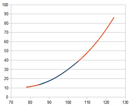
Figure 1: Estimation and Extrapolation of the Volatility Function

The blue part of the graph is the estimated function, and the red part is its extrapolation using the technique of Reproducing Kernel Hilbert Spaces (RKHS).

These LinkedIn results illustrate the usefulness of our new methodology for detecting bubbles in real time. Our methodology provides a solution to the problems stated by both Chairman Bernanke and President Dudley, and it is our hope that they will prove useful to regulators, policy makers, and industry participants alike.

Acknowledgement: The authors thank Peter Carr and Arun Verma for help in obtaining quickly the tick data for the stock LinkedIn.

The Empirical Test

In this section we first review the methodology contained in [6] to determine whether or not LinkedIn’s stock price is experiencing a bubble, and then we apply this methodology to LinkedIn minute by minute stock price tick data obtained from Bloomberg. We conclude that LinedIn’s stock is indeed experiencing a price bubble.

1.1 The Methodology

The methodology is based on studying the characteristics of LinkedIn’s stock price process. If LinkedIn’s stock price is experiencing a bubble, it can be shown [6] that the stock price’s volatility will be unusually large. Our empirical methodology validates whether or not LinkedIn’s stock volatility is large enough.

To perform this validation, we start by assuming that the stock price follows a stochastic differential equation of a form that makes it a diffusion in an incomplete market (see (2) below). The assumed stock price evolution is very general and fits most stock price processes reasonably well. For identifying a price bubble, the key characteristic of this evolution is that the stock price’s volatility $\sigma(S_{t})$ is a function of the level of the stock price.

Next, we use sophisticated methods to estimate the volatility coefficient $\sigma(x)$. Since the data is necessarily finite, we can estimate the values of $\sigma(x)$ only on the set of stock prices observed (which is a compact subset of $\mathbb{R}_{+}$) We use two methods to extend $\sigma$ to all of $\mathbb{R}_{+}$. One, we use parametric methods combined with a comparison theorem. Two, we use an indexed family of Reproducing Kernel Hilbert Spaces (RKHS) combined with an optimization over the index set to obtain the best possible extension given the data (this is a sort of bootstrap procedure).

This “knowledge of $\sigma(S_{t})$” then enables us to determine whether the stock price is a martingale or is a strict local martingale under any of an infinite collection of risk neutral measures. If it is a strict local martingale for all of the risk neutral measures (which corresponds to a certain calculus integral being finite by Feller’s test for explosions), then we can conclude that the stock price is undergoing a bubble. Otherwise, there is not a stock price bubble.

1.2 The Estimation

We assume that LinkedIn’s stock price is a diffusion of the form

$$dS_{t} = \sigma(S_{t})dW_{t}+b(S_{t},Y_{t})dt$$ (1)

$$dY_{t} = s(Y_{t})dB_{t}+g(Y_{t})dt$$ (2)

where $W$ and $B$ are independent Brownian motions. This model permits that under the physical probability measure, the stock price can have a drift that depends on additional randomness, making the market incomplete (see [6]). Nevertheless for this family of models, $S$ satisfies the following equation for every neutral measure:

$$dS_{t}=\sigma(S_{t})dW_{t}$$

Under this evolution, the stock price exhibits a bubble if and only if

$$\int_{a}^{\infty}\frac{x}{\sigma^{2}(x)}dx<\infty\ \ for\ all\ \ a>0.$$ (3)

We test to see if this integral is finite or not.

To perform this test, we obtained minute by minute stock price tick data for the 4 business days 5/19/2011 to 5/24/2011 from Bloomberg. There are exactly 1535 price observations in this data set. The time series plot of LinkedIn’s stock price is contained in Figure 2. The prices used are the open prices of each minute but the results are not sensitive to using open, high or lowest minute prices instead.

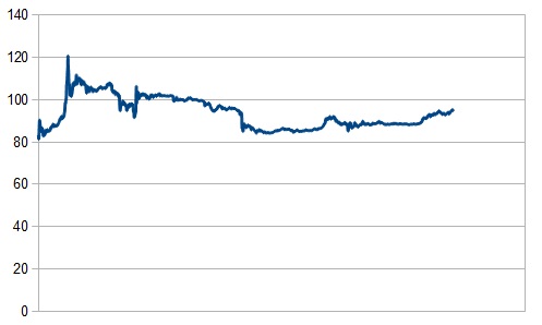
Figure 2: LinkedIn Stock Prices from 5/19/2011 to 5/24/2011.(The observation interval is one minute.)

The maximum stock price attained by LinkedIn during this period is $120.74 and the minimum price was $81.24. As evidenced in this diagram, LinkedIn experienced a dramatic price rise in its early trading. This suggests an unusually large stock price volatility over this short time period and perhaps a price bubble.

Our bubble testing methodology first requires us to estimate the volatility function $\sigma$ using local time based non-parametric estimators. We use two such estimators. We compare the estimation results obtained using both Zmirou’s estimator (see Theorem 1 in [4]) and the estimator developed in [4] (see Theorem 3 in the same reference). The implementation of these estimators requires a grid step $h_{n}$ tending to zero, such that $nh_{n}\rightarrow\infty$ and $nh_{n}^{4}\rightarrow 0$ for the former estimator, and $nh_{n}^{2}\rightarrow\infty$ for the later one. We choose the step size $h_{n}=\frac{1}{n^{\frac{1}{3}}}$ so that all of these conditions are simultaneously satisfied. This implies a grid of 7 points. The statistics are displayed in figure 3.

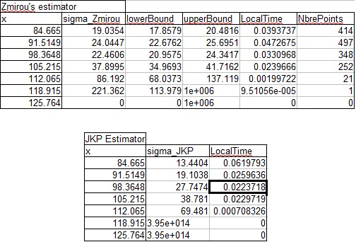
Figure 3: Non-parametric Volatility Estimates.

Since the neighborhoods of the grid points $118.915 and $125.764 are either not visited or visited only once, we do not have reliable estimates at these points. Therefore, we restrict ourselves to the grid containing only the first five points. We note that the last point in the new grid $112.065 still has only been visited very few times.

When using Zmirou’s estimator, confidence intervals are provided. The confidence intervals are quite wide. Given these observations, we apply our methodology twice. In the first test, we use a 5 point grid. In the second test, we remove the fifth point where the estimation is uncertain and we use a 4 point grid instead. The graph in figure 4 plots the estimated volatilities for the grid points together with the confidence intervals.

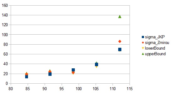
Figure 4: Non parametric Volatility Estimation Results.

The next step in our procedure is to interpolate the shape of the volatility function between these grid points. We use the estimations from our non parametric estimator with the 5 point grid case. For the volatility time scale, we let the 4 day time interval correspond to one unit of time. This scaling does not affect the conclusions of this paper. When interpolating one can use any reasonable method. We use both cubic splines and reproducing kernel Hilbert spaces as suggested in [4], subsection 5.2.3 item (ii). The interpolated functions are in figure 5.

From these,we select the kernel function $K_{1,\tau}$ as defined in Lemma 10 in [4], and we choose the parameter $\tau=6$.

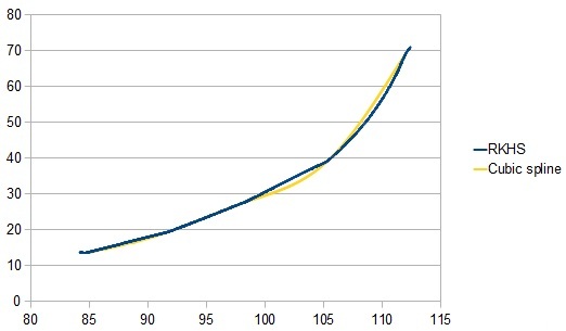
Figure 5: Interpolated Volatility using Cubic Splines and the RKHS Theory

The next step is to extrapolate the interpolated function $\sigma^{b}$ using the RKHS theory to the left and right stock price tails. Define $f(x)=\frac{1}{\sigma^{2}(x)}$ and define the Hilbert space

$$H_{n}=H_{n}\big{(}[0,\infty[\big{)}=\big{\{}f\in C^{n}\big{(}[0,\infty[\big{)}\mid\lim_{x\rightarrow\infty}x^{k}f^{(k)}(x)=0\text{ for all }0\leq k\leq n-1\big{\}}$$

where $n$ is the assumed degree of smoothness of $f$. We also need to define an inner product. A smooth reproducing kernel $q^{RP}(x,y)$ can be constructed explicitly (see Proposition 2 in [4]) via the choice

$$\langle f,g\rangle_{n,m}=\int_{0}^{\infty}\frac{y^{n}f^{(n)}(y)}{n!}\frac{y^{n}g^{(n)}(y)}{n!}\frac{dy}{w(y)}$$

where $w(y)=\frac{1}{y^{m}}$ is an asymptotic weighting function. We consider the family of RKHS $H_{n,m}=(H_{n},\langle,\rangle_{n,m})$, in which case the explicit form of $q_{n,m}^{RP}$ is provided in Proposition 2 in [4] in terms of the Beta and the Gauss’s hypergeometric functions.

For $n\in\{1,2\}$ fixed, we construct our extrapolation $\sigma=\sigma_{m}$ as in [4], 5.2.3 item (iv), by choosing the asymptotic weighting function parameter $m$ such that $f_{m}=\frac{1}{\sigma_{m}^{2}}$ is in $H_{n,m}$, $\sigma_{m}$ exactly matches the points obtained from the non parametric estimation, and $\sigma_{m}$ is as close (in norm 2) to $\sigma^{b}$ on the last third of the bounded interval where $\sigma^{b}$ is defined. Because of the observed kink and the obvious change in the rate of increase of $\sigma^{b}$ at the forth point, we choose $n=1$ in our numerical procedure. The result is shown in figure 6.

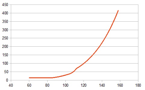
Figure 6: RKHS Based Extrapolation of $\sigma^{b}$

We obtain $m=9.42$.

From Proposition 3 in [4], the asymptotic behavior of $\sigma$ is given by

$$\lim_{x\rightarrow\infty}x^{m+1}f(x)=n^{2}B(m+1,n)\sum_{i=1}^{M}c_{i}$$

where $M=5$ is the number of observations available, $B$ is the Beta function, and the coefficients $(c_{i})_{1\leq i\leq M}$ are obtained by solving the system

$$\sum_{i=1}^{M}c_{i}q_{n,m}^{RP}(x_{i},x_{k})=f(x_{k})\text{ for all }1\leq k\leq M$$

where $(x_{i})_{1\leq i\leq M}$ is the grid of the non parametric estimation, $f(x_{k})=\frac{1}{\sigma^{2}(x_{k})}$ and $\sigma(x_{k})$ is the value at the grid point $x_{k}$ obtained from the non-parametric estimation procedure. This implies that $\sigma$ is asymptotically equivalent to a function proportional to $x^{\alpha}$ with $\alpha=\frac{1+m}{2}$, that is $\alpha=5.21$. This value appears very large, however, the proportionality constant is also large. The $c_{i}$’s are automatically adjusted to exactly match the input points $(x_{i},f(x_{i}))_{1\leq i\leq M}$.

We plot below the functions with different asymptotic weighting parameters $m$ obtained using the RKHS extrapolation method, without optimization. All the functions exactly match the non-parametrically estimated points.

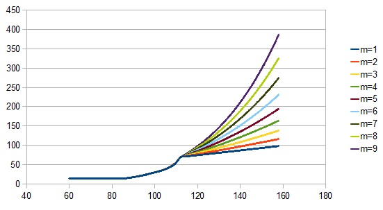
Figure 7: Extrapolated Volatility Functions using Different Reproducing Kernels

The asymptotic weighting function’s parameter $m=9.42$ obtained by optimization appears in figure 7 to be the estimate most consistent (within all the functions, in any Hilbert Space of the form $H_{1,m}$, that exactly match the input data) with a ”natural” extension of the behavior of $\sigma^{b}$ to $\mathbb{R}^{+}$. The power $\alpha=5.21$ implies then that LinkedIn stock price is currently exhibiting a bubble.

Since there is a large standard error for the volatility estimate at the end point $112.065, we remove this point from the grid and repeat our procedure. Also, the rate of increase of the function between the last two last points appears large, and we do not want the volatility’s behavior to follow solely from this fact. Hence, we check to see if we can conclude there is a price bubble based only on the first 4 reliable observation points. We plot in figure 8 the function $\sigma^{b}$ (in blue) and its extrapolation to $\mathbb{R}^{+}$, $\sigma$ (in red).

Figure 8: RKHS based Extrapolation of $\sigma^{b}$

Now $M=4$. With this new grid, we can assume a higher regularity $n=2$ and we obtain, after optimization, $m=7.8543$. This leads to the power $\alpha=4.42715$ for the asymptotic behavior of the volatility. Again, although this power appears to be high given the numerical values $(x_{k},f(x_{k}))_{1\leq k\leq 4}$, the coefficients $(c_{i})_{1\leq i\leq 4}$ and hence the constant of proportionality are adjusted to exactly match the input points. The extrapolated function obtained is the most consistent (within all the functions, in any $H_{2,m}$, that exactly match the input data) in terms of extending ’naturally’ the behavior of $\sigma^{b}$ to $\mathbb{R}^{+}$. Again, we can conclude that there is a stock price bubble.

References

- [1] Ben Bernanke, Senate Confirmation Hearing, December 2009. This is quoted in many places; one example is Dealbook, edited by Andrew Ross Sorkin, January 6, 2010.
- [2] Julie Creswell, Analysts Are Wary of LinkedIn’s Stock Surge, New York Times Digest, p. 4, Monday, May 23, 2011.
- [3] Jacob Goldstein, interview with William Dudley, the President of the New York Federal Reserve; in Planet Money, April 9, 2010
- [4] R. Jarrow, Y. Kchia, and P. Protter, How to Detect an Asset Bubble (February 2011). Johnson School Research Paper Series No. 28-2010. Available at SSRN: http://ssrn.com/abstract=1621728
- [5] R. Jarrow, P. Protter and K. Shimbo, Asset Price Bubbles in Complete Markets, Advances in Mathematical Finance, Springer-Verlag, M.C. Fu et al, editors, 2007, 97–122.
- [6] R. Jarrow, P. Protter and K. Shimbo, Asset Price Bubbles in Incomplete Markets, Mathematical Finance, 20, 2010, 145-185.