Viability of the exact tri-bimaximal mixing at $M_{GUT}$ in $SO(10)$

Abstract

General structures of the charged lepton and the neutrino mixing matrices leading to tri-bimaximal leptonic mixing are determined. These are then integrated into an $SO(10)$ model within which detailed fits to fermion masses and mixing angles are given. It is shown that one can obtain excellent fits to all the fermion masses and quark mixing angles keeping tri-bimaximal leptonic mixing intact. Different perturbations to the basic structure are considered and those which can or which cannot account for the recent T2K and MINOS results on the reactor mixing angle $\theta_{13}^{l}$ are identified.

I Introduction

The Tri-bimaximal (TBM) leptonic mixing hs provides an important clue in search of possible flavour structure af governing the leptonic masses and mixing angles. It predicts $\sin^{2}\theta_{12}^{l}=1/3$ and $\sin^{2}\theta_{23}^{l}=1/2$ respectively for the solar and the atmospheric mixing angles both of which agree nearly within 1$\sigma$ with the latest global analysis fogli ; valle of the neutrino oscillation data. TBM also predicts vanishing reactor mixing angle $\theta_{13}^{l}$. This can be reconciled with the latest T2K t2k (MINOS minos ) results at 2.5$\sigma$ (1.6$\sigma)$ and with the global analysis fogli ; valle at about 3$\sigma$. This suggests that the TBM may be a good zeroth order approximation which needs perturbations affecting mainly the reactor mixing angle $\theta_{13}^{l}$. While such perturbations may arise from some underlying flavor symmetry, see modelflavor for examples, it would be more appropriate if some independent mechanism like grand unified theory (GUT) moh:t2k governs these perturbations. We wish to analyze here the TBM structure and perturbations to it within a grand unified model based on $SO(10)$ gauge symmetry.

Incorporating the tri-bimaximal mixing into GUTs, particularly based on the $SO(10)$ gauge group is quite challenging, see sm for some examples. Since all fermions in a given generation are unified into a single $16$ dimensional irreducible representation of $SO(10)$, imposition of the TBM structure on the leptonic mass matrices also constrains the quark mass matrices. It is not clear if the requirement of the exact tri-bimaximal mixing among leptons would be consistent with a precise description of the quark masses and mixing. We suggest a general method of incorporating the exact TBM structure within $SO(10)$ and use it to obtain quantitative description of the fermion masses and mixing.

Our approach is purely phenomenological. We do not use any flavour symmetry but determine the most general structure of the leptonic mixing matrices required for obtaining the tri-bimaximal mixing. We then try to integrate this structure into $SO(10)$ and discuss numerical fits to the quark masses and mixing leaving the TBM intact. Then we discuss perturbations to the basic structure and their effects on observables.

II Leptonic mixing matrices and TBM

We shall derive general forms for the neutrino mass matrix $M_{\nu}$ and the left handed charged lepton mixing matrix $U_{l}$ which lead in the flavour basis to a neutrino mass matrix ${\cal M}_{\nu f}~{}$exhibiting the TBM structure. We define the TBM structure for ${\cal M}_{\nu f}~{}$as follows:

$${\cal M}_{\nu f}=\frac{1}{3}\left(\begin{array}[]{ccc}2f_{1}+f_{2}&f_{2}-f_{1}&f_{2}-f_{1}\\ f_{2}-f_{1}&\frac{1}{2}(f_{1}+2f_{2}+3f_{3})&\frac{1}{2}(f_{1}+2f_{2}-3f_{3})\\ f_{2}-f_{1}&\frac{1}{2}(f_{1}+2f_{2}-3f_{3})&\frac{1}{2}(f_{1}+2f_{2}+3f_{3})\\ \end{array}\right)~{},$$ (1)

where $f_{1,2,3}$ are complex neutrino masses. This matrix is diagonalized by

$$U_{PMNS}=O_{TBM}Q~{},$$ (2)

where $Q$ is a diagonal phase matrix and

$$O_{TBM}=\left(\begin{array}[]{ccc}\sqrt{\frac{2}{3}}&\frac{1}{\sqrt{3}}&0\\ -\frac{1}{\sqrt{6}}&\frac{1}{\sqrt{3}}&-\frac{1}{\sqrt{2}}\\ -\frac{1}{\sqrt{6}}&\frac{1}{\sqrt{3}}&\frac{1}{\sqrt{2}}\\ \end{array}\right)$$ (3)

A more general definition of TBM structure would be to replace ${\cal M}_{\nu f}$ and $U_{PMNS}$ above by $P_{l}{\cal M}_{\nu f}P_{l}$ and $P_{l}^{*}U_{PMNS}$, where $P_{l}$ denotes a diagonal phase matrix. Since $P_{l}$ can be rotated away by redefining the charged lepton fields, we shall refer to TBM structure as the one defined by Eqs. (1,2).

It is known lam that ${\cal M}_{\nu f}~{}$in Eq. (1) is invariant under a $Z_{2}\times Z_{2}$ symmetry. The elements of the $Z_{2}\times Z_{2}$ are defined as

$$\begin{array}[]{cc}S_{2}=\dfrac{1}{3}\left(\begin{array}[]{ccc}-1&2&2\\ 2&-1&2\\ 2&2&-1\\ \end{array}\right)~{}~{}~{}{\rm and{}{}{}}&S_{3}=\left(\begin{array}[]{ccc}1&0&0\\ 0&0&1\\ 0&1&0\\ \end{array}\right).\end{array}$$ (4)

and satisfy

$$S_{2,3}^{T}{\cal M}_{\nu f}S_{2,3}={\cal M}_{\nu f}~{}$$ (5)

We shall exploit this $Z_{2}\times Z_{2}$ invariance in arriving at the structure of $U_{l}$. As noted in ab , one can always choose a specific basis in which $M_{\nu}$ exhibits the TBM structure and is thus invariant under $Z_{2}\times Z_{2}$:

$$S_{2,3}^{T}M_{\nu}S_{2,3}=M_{\nu}~{}$$ (6)

If $M_{\nu}^{\prime}$ in an arbitrary basis is not invariant under $Z_{2}\times Z_{2}$ then one can go to a new basis with $M_{\nu}=U^{T}M_{\nu}^{\prime}U$ and choose $U$ in such a way that

$$U_{\nu}^{T}M_{\nu}U_{\nu}=D_{\nu}~{},$$ (7)

with $D_{\nu}$ a diagonal matrix with real positive elements and

$$U_{\nu}\equiv O_{TBM}P~{}.$$ (8)

$P$ being a general diagonal phase matrix. Let $U_{l}$ denote the mixing matrix among the left handed charged leptons in a basis in which $M_{\nu}$ is $Z_{2}\times Z_{2}$ symmetric. If such a defined $U_{l}$ itself is $Z_{2}\times Z_{2}$ symmetric, i.e. satisfies

$$S_{2,3}^{T}U_{l}S_{2,3}=U_{l}~{}$$ (9)

then ${\cal M}_{\nu f}~{}$will also satisfy Eq. (5) and thus would exhibit the TBM structure of Eq. (1). This follows trivially from the definition

$${\cal M}_{\nu f}=U_{l}^{T}M_{\nu}U_{l}~{},$$ (10)

after using Eqs. (6,9). Thus the $Z_{2}\times Z_{2}$ invariance of $U_{l}$ is sufficient to ensure the TBM for ${\cal M}_{\nu f}~{}$.

Above equation allows us to determine TBM preserving class of $U_{l}$ in a basis with $M_{\nu}$ satisfying Eq. (6). $S_{3}$ invariance corresponds to imposing the $\mu$-$\tau$ interchange symmetry on $U_{l}$. The $S_{2}$ invariance further requires $U_{l}^{T}=U_{l}$ and that the sum of elements in each of its raw must be equal. Such a $U_{l}$ can be parameterized as

$$U_{l}=e^{i\alpha}P_{l}\tilde{U_{l}}P_{l}~{},$$ (11)

where $P_{l}={\rm diag.}(1,e^{i\beta},e^{i\beta})$ is a diagonal phase matrix and

$$\tilde{U_{l}}=\left(\begin{array}[]{ccc}c_{\theta}&\frac{s_{\theta}}{\sqrt{2}}&\frac{s_{\theta}}{\sqrt{2}}\\ \frac{s_{\theta}}{\sqrt{2}}&-\frac{1}{2}(c_{\theta}+e^{i\delta})&-\frac{1}{2}(c_{\theta}-e^{i\delta})\\ \frac{s_{\theta}}{\sqrt{2}}&-\frac{1}{2}(c_{\theta}-e^{i\delta})&-\frac{1}{2}(c_{\theta}+e^{i\delta})\end{array}\right),$$ (12)

with $\tan\theta=-2\sqrt{2}\cos\beta$. $U_{l}$ is thus fully determined by three phase angles $\alpha,\beta$ and $\delta$.

The form of $U_{l}$ as given above is the most general one required in order to obtain TBM in the basis with $M_{\nu}$ satisfying Eq. (6). The generality is proved by noticing that the $Z_{2}\times Z_{2}$ invariance of $U_{l}$ is also necessary if ${\cal M}_{\nu f}~{}$is to exhibit the TBM structure. This follows in a straightforward manner. Assume that ${\cal M}_{\nu f}~{}$has TBM structure of Eq. (1). The $U_{PMNS}$ matrix in this case can be chosen to have the form in Eq. (2). Since $U_{l}=U_{\nu}U_{PMNS}^{\dagger}$, it has the following form in the basis specified by Eq. (8):

$$U_{l} = O_{TBM}PQ^{*}O^{T}_{TBM}~{},$$ (16)

$$= \frac{1}{3}\left(\begin{array}[]{ccc}2p_{1}+p_{2}&p_{2}-p_{1}&p_{2}-p_{1}\\ p_{2}-p_{1}&\frac{1}{2}(p_{1}+2p_{2}+3p_{3})&\frac{1}{2}(p_{1}+2p_{2}-3p_{3})\\ p_{2}-p_{1}&\frac{1}{2}(p_{1}+2p_{2}-3p_{3})&\frac{1}{2}(p_{1}+2p_{2}+3p_{3})\end{array}\right)~{},$$

where $p_{i}$ denote the elements of the diagonal phase matrix $PQ^{*}$. Interestingly, the above $U_{l}$ is obtained from the general TBM ${\cal M}_{\nu f}~{}$Eq. (1), by replacing the neutrino masses with the phases $p_{i}$ and like ${\cal M}_{\nu f}~{}$such a $U_{l}$ is automatically $Z_{2}\times Z_{2}$ symmetric. Thus Eq. (9) also becomes necessary for the $Z_{2}\times Z_{2}$ invariance of ${\cal M}_{\nu f}~{}$. Eq. (16) provides an alternative parametrization of $U_{l}$. It reduces to the earlier parametrization in Eq. (12) with the definition

$$p_{1} = -e^{i(\alpha+\beta-\eta)},$$

$$p_{2} = ~{}e^{i(\alpha+\beta+\eta)},$$

$$p_{3} = -e^{i(\alpha+2\beta+\delta)},$$ (17)

with $\cos\eta=-3c_{\theta}\cos\beta$ and $\sin\eta=-c_{\theta}\sin\beta$.

We note that the $U_{\nu}$ and $U_{l}$ in Eqs. (8,11) are defined up to a simultaneous redefinition $U_{\nu}\rightarrow UU_{\nu}$ and $U_{l}\rightarrow UU_{l}$. In addition, $U_{l}$ can also be multiplied by an arbitrary phase matrix from the right. Since $P_{l}$ is arbitrary, the $U_{l}$ in some model may not appear to have the $Z_{2}\times Z_{2}$ invariance even in a basis with $U_{\nu}$ chosen as in Eq. (8). But the above exercise shows that $U_{l}$ can always be chosen to have the TBM form by appropriate rephasing of the charged lepton fields.

The above reasoning can be applied to more general patterns of mixing and not just to TBM. The key role in this construction is played by the fact that one can always choose a basis in which $M_{\nu}$ is $Z_{2}\times Z_{2}$ symmetric. This follows from the fact that the $Z_{2}\times Z_{2}$ symmetry does not put any restrictions on the neutrino masses but only on the structure of mixing. As long as the neutrino mass matrices obey such “mass-independent” symmetries, the above construction of determining the most general $U_{l}$ can be carried through. One can indeed define lam an appropriate $Z_{2}\times Z_{2}$ symmetry corresponding to every mixing pattern and then impose this symmetry on $U_{l}$ to obtain the desired mixing structure in the flavour basis. As an example, in case of the $\mu$-$\tau$ symmetry, one can always choose a basis in which $M_{\nu}$ is $\mu$-$\tau$ symmetric. Then requiring that $U_{l}$ also be $\mu$-$\tau$ symmetric, we arrive at a general forms for $U_{l}$ and $M_{\nu}$ which lead to a $\mu$-$\tau$ symmetric ${\cal M}_{\nu f}~{}$:

$$\begin{array}[]{cc}M_{\nu}=\left(\begin{array}[]{ccc}X&A&A\\ A&B&C\\ A&C&B\\ \end{array}\right)&~{};~{}~{}~{}U_{l}=e^{i\alpha}P_{lL}\tilde{U_{l}}P_{lR}{}\end{array}$$ (18)

where $P_{lL,R}={\rm diag.}(1,e^{i\beta_{L,R}},e^{i\beta_{L,R}})$ and $\tilde{U_{l}}$ has the same form of Eq. (12) but now $\theta$ is an independent parameter and is not a function of $\beta$ as before.

III $SO(10)$ model and TBM

We now integrate the above leptonic structures into an $SO(10)$ model. We make the following assumptions which lead to simplification and allows us to obtain quantitative description. We (1) consider a supersymmetric $SO(10)$ model with the Higgs transforming as $10,\overline{126},120$ representations of $SO(10)$ (2) impose the generalized parity as in moh120 ; grimus1 ; mutau ; ab ; jp leading to Hermitian mass matrices and (3) assume that the dominant contribution to $M_{\nu}$ is a type-II seesaw, i.e. linear in the $\overline{126}$ Yukawa coupling. The last assumption with its attractive consequences is made in a number of $SO(10)$ models ab ; moh120 ; minimal ; nonminimal . The type-II dominance may be achieved by adding more Higgs fields. The type-I contribution can be suppressed by pushing the $B-L$ breaking scale high while the type -II contribution can be relatively enhanced if the Higgs triplet remains below the GUT scale. The latter spoils the gauge coupling unification. It was pointed out in moh54 that breaking $SO(10)$ to $SU(5)\times U(1)$ around $10^{17}$ GeV can suppress the type-I contribution and presence of $54$ plet can allow a complete multiplet transforming as 15 in $SU(5)$ to remain light. One can achieve in this way the type-II dominance without sacrificing the gauge coupling unification. The same phenomena was analyzed subsequently goran2 in a model with fields transforming as $54+45$ (instead of the standard $210$) and having a $120$ plet of Higgs. The fields $54+45$ required to achieve the type-II dominance do not effect the fermion masses and the fermion sector can be the same as considered here.

The fermion mass relations in this case after electroweak symmetry breaking can be written in their most general forms as grimus1 ; mutau ; jp :

$$M_{d} = H+F+iG~{},$$

$$M_{u} = r(H+sF+it_{u}~{}G~{}),$$

$$M_{l} = H-3F+~{}it_{l}~{}G~{},$$

$$M_{D} = r(H-3sF+it_{D}~{}G~{}),$$

$$M_{L} = r_{L}F~{},$$

$$M_{R} = r_{R}^{-1}F.$$ (19)

where ($G$) $H$, $F$ are real (anti)symmetric matrices. $r,s,t_{l},t_{u},t_{D},r_{L},r_{R}$ are dimensionless real parameters. The effective neutrino mass matrix for three light neutrinos resulting after the seesaw mechanism can be written as

$$M_{\nu}=r_{L}F-r_{R}M_{D}F^{-1}M_{D}^{T}\equiv M_{\nu}^{II}+M_{\nu}^{I}~{}.$$ (20)

The first term proportional to $F$ denotes type-II seesaw contribution. In the numerical analysis that follows, we shall assume that $M_{\nu}$ is entirely given by this term and subsequently analyze the effect of a small type-I corrections on the numerical solution found.

We can always rotate the 16-plet fermions in generation space in such a way that $M_{\nu}\propto F$ is diagonalized by the TBM matrix.

$$F\rightarrow R^{T}FR=F_{TBM}\equiv O_{TBM}~{}{\rm Diag.}(f_{1},f_{2},f_{3})~{}O_{TBM}^{T}$$ (21)

where $f_{i}$ are now real eigenvalues of $F$ and the $O_{TBM}$ is given by Eq. (3). The matrix ($G$)$H$ maintains its (anti)symmetric form in such basis and we use the same label for them in the rotated basis. In case of type-II seesaw dominance, the light neutrino mass matrix $M_{\nu}=r_{L}F_{TBM}$ has the form given on the RHS of Eq. (1). The model has altogether 17 independent real parameters (3 in $F_{TBM}$, 6 in $H$, 3 in $G$, $r$, $s$, $t_{u}$, $t_{l}$ and $r_{L}$) which determine the entire 22 low energy observables of the fermion mass spectrum. Some of these parameters can be fixed by the known values of observables directly. As noted in jp , the $SO(10)$ relation for the charged lepton mass matrix in Eq. (III) can be rewritten as

$$H+it_{l}G=V_{l}D_{l}V_{l}^{\dagger}+3F_{TBM}~{},$$ (22)

where $D_{l}$ is a diagonal charged lepton mass matrix. Since $H$ and $G$ are real, the real and imaginary parts of the RHS separately determine $H$ and $t_{l}G$ in terms of the charged lepton masses, parameters of $F_{TBM}$ and $V_{l}$. $V_{l}$ is a unitary matrix that diagonalizes $M_{l}$ and contains nine free parameters in the most general situation. One can suitably write $V_{l}=\tilde{V_{l}}P$ where $P$ is diagonal phase matrix and $\tilde{V_{l}}$ contains six real parameters. From Eq. (22), it is easy to see that the phase matrix $P$ does not play any role in determining $H$ and $G$ and can be removed. So the nine real parameters of LHS can be related to six real parameters of $\tilde{V_{l}}$, three charged lepton masses and parameters of $F_{TBM}$ in Eq. (22). This fixing helps us in numerical analysis as we will see in the next subsection.

We shall present numerical analysis in two different cases. (A) Corresponding to the most general $V_{l}$ (B) with $V_{l}=U_{l}$ given as in Eqs. (11,12). The case (A) has already been studied numerically in moh120 ; ab ; jp . We refine this analysis using a different numerical procedure and taking into account the results of the most recent global fits fogli to neutrino data. This also serves as a benchmark with which to compare the case (B) which leads to the exact TBM at $M_{GUT}$.

III.1 Numerical Analysis: The most general case

We study the viability of Eq. (III) with the experimentally observed values of fermion masses and mixing angles through numerical analysis. For this, we construct a $\chi^{2}$ function defined as

$$\chi^{2}=\sum_{i}\left(\frac{P_{i}-O_{i}}{\sigma_{i}}\right)^{2}~{}$$ (23)

where the sum runs over different observables. $P_{i}$ denote the theoretical values of observables determined by the expressions given in Eq. (III) and $O_{i}$ are the experimental values extrapolated to the GUT scale. $\sigma_{i}$ denote the 1$\sigma$ errors in $O_{i}$. Our choice of the input values of quark and lepton masses and quark mixing angles are the same as used in ab . In this data set, the charged fermion masses at the GUT scale are dasparida obtained from the low energy values using MSSM and $\tan\beta=10$. We use the input values of lepton mixing angles from fogli which includes results from T2K and MINOS. The effect of the RG evolution on the quark mixing angles is known to be negligible. This is also true for the lepton mixing angles in case of the hierarchical neutrino spectrum. We assume such hierarchy in neutrino masses and therefore the input values of the quark mixing angles, CP phase and neutrino parameters we use correspond to their values at low energy. We reproduce all these input values in Table 1 for convenience of the reader.

$\begin{array}[]{|c|c||c|c|}\hline\cr\vrule\lx@intercol\hfil\text{GUT scale values with propagated uncertainty}\hfil\lx@intercol\vrule\lx@intercol\\ \hline\cr m_{d}(\text{MeV})&1.24\pm 0.41&\Delta m^{2}_{sol}(\text{eV${}^{2}$})&(7.58\pm 0.22)\times 10^{-5}\\ m_{s}(\text{MeV})&21.7\pm 5.2&\Delta m^{2}_{atm}(\text{eV${}^{2}$})&(2.35\pm 0.12)\times 10^{-3}\\ m_{b}(\text{GeV})&1.06^{+0.14}_{-0.09}&\sin\theta_{12}^{q}&0.2243\pm 0.0016\\ m_{u}(\text{MeV})&0.55\pm 0.25&\sin\theta_{23}^{q}&0.0351\pm 0.0013\\ m_{c}(\text{GeV})&0.210\pm 0.021&\sin\theta_{13}^{q}&0.0032\pm 0.0005\\ m_{t}(\text{GeV})&82.4^{+30.3}_{-14.8}&\sin^{2}\theta_{12}^{l}&0.306^{+0.018}_{-0.015}\\ m_{e}(\text{MeV})&0.3585\pm 0.0003&\sin^{2}\theta_{23}^{l}&0.42^{+0.08}_{-0.03}\\ m_{\mu}(\text{MeV})&75.672\pm 0.058&\sin^{2}\theta_{13}^{l}&0.021^{+0.007}_{-0.008}\\ m_{\tau}(\text{GeV})&1.2922\pm 0.0013&J_{CP}&(2.2\pm 0.6)\times 10^{-5}\\ \hline\cr\end{array}$

Table 1: Input values for quark and leptonic masses and mixing angles in the MSSM extrapolated at $M_{GUT}=2\times 10^{16}$ GeV for $\tan\beta=10$ which we use in our numerical analysis.

We fit the above data to the fermion mass relations (III) predicted in the model by numerically minimizing the $\chi^{2}$ function. As already mentioned above, this exercise has been done in ab recently and a very good fit corresponding to $\chi^{2}_{min}=0.127$ is found. We repeat the same analysis because of the following differences in our fitting procedure and because of the emergence of new results on $\theta_{13}^{l}$ t2k ; minos .

• Compared to other observables, the charged lepton masses are known very precisely with extremely small errors in their measurements. Instead of fitting them through $\chi^{2}$ minimization, we use their central values as inputs on the RHS of Eq. (22). Because of this, our definition of the $\chi^{2}$ function in Eq. (23) does not include the charged lepton masses in it.

• We also use the central value of the solar to the atmospheric mass squared difference ratio as an input and use it to fix $f_{3}$ through the following relation:

  $$f_{3}=f_{2}\left(\dfrac{\Delta m^{2}_{atm}}{\Delta m^{2}_{sol}}+\left(1-\dfrac{\Delta m^{2}_{atm}}{\Delta m^{2}_{sol}}\right)\left(\dfrac{f_{1}}{f_{2}}\right)^{2}\right)^{1/2}.$$ (24)

  After obtaining the solution, the overall scale of neutrino masses $r_{L}$ at the minimum is determined by using the atmospheric scale as a normalization.

As a result of these simplifications, the $\chi^{2}$ function in our approach includes only 13 observables, 6 quark masses, 3 quark mixing angles, a CKM phase and 3 lepton mixing angles. These are complex nonlinear functions of 12 real parameters (2 in $F_{TBM}$, 6 in $V_{l}$, $r$, $s$, $t_{l}$ and $t_{u}$). This $\chi^{2}$ is numerically minimized using the function minimization tool MINUIT. The results of our analysis are shown in column A in Table 2.

$\begin{array}[]{|c||c|c||c|c||c|c|}\hline\cr&\vrule\lx@intercol\hfil\text{\bf Case A}\hfil\lx@intercol\vrule\lx@intercol\vrule\lx@intercol&\vrule\lx@intercol\hfil\text{\bf Case B1}\hfil\lx@intercol\vrule\lx@intercol\vrule\lx@intercol&\vrule\lx@intercol\hfil\text{\bf Case B2}\hfil\lx@intercol\vrule\lx@intercol\\ \hline\cr\text{Observables}&\text{Fitted value}&\text{Pull}&\text{Fitted value}&\text{Pull}&\text{Fitted value}&\text{Pull}\\ \hline\cr m_{d}[{\rm MeV}]&1.2339&-0.0148738&1.22098&-0.0463899&1.02686&-0.519852\\ m_{s}[{\rm MeV}]&21.7214&0.00411949&21.9922&0.0561874&22.0058&0.058806\\ m_{b}[{\rm GeV}]&1.06614&0.0438763&1.16345&0.738942&1.2842&1.60145\\ m_{u}[{\rm MeV}]&0.550018&0.000073755&0.550234&0.000936368&0.550787&0.00314771\\ m_{c}[{\rm GeV}]&0.209977&-0.00111886&0.209952&-0.00230315&0.210481&0.0229054\\ m_{t}[{\rm GeV}]&82.5278&0.00421748&82.5855&0.00612198&81.7487&-0.0440052\\ m_{e}[{\rm MeV}]&0.3585&-&0.3585&-&0.3585&-\\ m_{\mu}[{\rm MeV}]&75.672&-&75.672&-&75.672&-\\ m_{\tau}[{\rm GeV}]&1.2922&-&1.2922&-&1.2922&-\\ \left(\dfrac{\Delta m^{2}_{sol}}{\Delta m^{2}_{atm}}\right)&0.0323&-&0.031875&-&0.031875&-\\ \sin\theta_{12}^{q}&0.224299&-0.000688878&0.2243&0.0002182&0.224303&0.0019076\\ \sin\theta_{23}^{q}&0.0351032&0.00246952&0.0350951&-0.0038047&0.0351294&0.022597\\ \sin\theta_{13}^{q}&0.00320513&0.0102511&0.00319436&-0.0112796&0.0031749&-0.0502087\\ \sin^{2}\theta_{12}^{l}&0.306119&0.00660722&\textbf{0.3333}&-&\textbf{0.3333}&-\\ \sin^{2}\theta_{23}^{l}&0.418475&-0.0508353&\textbf{0.5}&-&\textbf{0.5}&-\\ \sin^{2}\theta_{13}^{l}&0.0207708&-0.0286467&\textbf{0}&-&\textbf{0}&-\\ J_{CP}&2.19\times 10^{-5}&-0.0183401&2.21\times 10^{-5}&0.0194165&2.25\times 10^{-5}&0.0845729\\ \delta_{MNS}&\textbf{282.396}&-&-&-&-&-\\ \alpha_{1}&\textbf{142.975}&-&\textbf{160.829}&-&\textbf{180}&-\\ \alpha_{2}&\textbf{22.4851}&-&\textbf{318.593}&-&\textbf{0}&-\\ r_{L}&6.89\times 10^{-10}&-&9.82\times 10^{-10}&-&3.53\times 10^{-9}&-\\ \hline\cr\hline\cr\chi^{2}_{min}&&\textbf{0.0061}&&\textbf{0.5519}&&\textbf{2.8510}\\ \hline\cr d_{FT}&&28751&&88546&&31171\\ d_{Data}&&220&&200&&200\\ \hline\cr\end{array}$

Table 2: Best fit solutions for fermion masses and mixing obtained assuming type-II seesaw dominance in the SUSY $SO(10)$ model with $10+\overline{126}+120$ Higgs. Various observables and their pulls at the minimum are shown for three different cases correspond to (A) the general (non TBM) leptonic mixing, (B1) Exact TBM leptonic mixing with $U_{l}$ of Eqs. (11,12) and (B2) Exact TBM leptonic mixing with diagonal $M_{l}$ and $t_{l}=0$ (See the discussions in the text for more details). The predictions of different approaches are shown in boldface.

We obtain an excellent fit corresponding to $\chi^{2}_{min}=0.0061$ which is significantly better than $\chi^{2}_{min}=0.127$ obtained in ab using different procedure and different data set. Parameters obtained for the best fit solution are shown in Appendix. All the observables are fitted within the 0.05$\sigma$ deviation from their central values. The solution at its minimum almost reproduces the central value of $\sin^{2}\theta_{13}^{l}$ obtained in the global fit fogli . We also determine a parameter $d_{FT}$ introduced in ab which quantitatively measures the amount of fine-tuning needed in the parameters for obtained fit when compared with $d_{Data}$ which is a similar parameter obtained from the data only. From our fit, we obtain $d_{FT}\sim 2.9\times 10^{4}$ compared to $d_{Data}\sim 220$. These parameters depend on the definition of $\chi^{2}$ and since we do not include the charged lepton masses -which have very small errors- in our $\chi^{2}$, both the parameters $d_{FT}$ and $d_{Data}$ are an order of magnitude smaller than ab . However the ratio $d_{Data}/d_{FT}\sim 7.6\times 10^{-3}$ obtained from our fit is almost similar to $d_{Data}/d_{FT}\sim 8\times 10^{-3}$ obtained in ab which shows that both of the solutions need substantial level of fine tunings in the model parameters.

III.2 Numerical Analysis: Exact TBM

After discussion of the above general case, we now specialize to the case of the exact TBM. This case is of considerable theoretical interest since it can point to some underlying symmetry existing at $M_{GUT}$. We can implement the exact TBM in a model independent way by choosing $V_{l}=U_{l}$ in Eq. (22). With this choice, all the leptonic mixing angles get fixed to their TBM values. Also the central value of the ratio of the solar to the atmospheric (mass)² differences is used as input and a parameter $r_{L}$ is determined at the minimum by using the atmospheric scale. Thus the $\chi^{2}$ function in Eq. (23) now involves only observables in the quark sector. As already discussed, $U_{l}$ in Eq. (11,12) is parameterized by three phase angles $\alpha,\beta$ and $\delta$. An overall phase $\alpha$ is irrelevant for the physical observables and can be removed. This leaves only 8 real parameters (2 in $F_{TBM}$, 2 in $U_{l}$, $r$, $s$, $t_{l}$ and $t_{u}$) which are fitted to the 10 observables in the quark sector by minimizing the $\chi^{2}$. The results are shown in column B1 in Table 2. The obtained fit corresponds to $\chi^{2}_{min}=0.552$ ($\chi^{2}_{min}/{\rm d.o.f.}=0.276$). Only the fitted value of $m_{b}$ deviates slightly from the central value with a $0.74\sigma$ pull. All the remaining observables are fitted within $0.06\sigma$. A set of parameters obtained for this solutions are shown in Appendix. The fit obtained here is not significantly different from the general case discussed before showing that all the fermion masses and mixing angles can be nicely reproduced along with the exact TBM within the $SO(10)$ framework discussed here.

Before we discuss possible perturbations in TBM pattern, let us discuss a very special case corresponding to a diagonal $M_{l}$. This corresponds to $U_{l}$ coinciding with an identity matrix and is a special case of Eq. (11,12) with $\beta=\frac{\pi}{2}$ and $\delta=0$. Since $M_{l}$ is real and diagonal in this case, $t_{l}G$ must vanish in Eq. (22). If $G=0$ then the quark mass matrices also become real and there is no room for CP violation. The viable scenario must therefore have nonzero $G$ and hence $t_{l}=0$. As a result, unlike before, the three parameters in $G$ do not get determined from $M_{l}$, see, Eq. (22) and remain free. They can be fitted from the quark sector observables. We carried out a separate numerical analysis for this particular case and the results are shown in column B2 in Table 2. The fit obtained gives relatively large $\chi^{2}_{min}=2.85$ ($\chi^{2}_{min}/{\rm d.o.f.}=1.43$) with more than 1$\sigma$ deviation in the bottom quark mass. Although the obtained $\chi^{2}_{min}$ is statistically acceptable at 90% confidence level, it is not as good as the previous one and we shall not consider this case with $U_{l}=I$ any further.

IV Perturbed TBM

The TBM is an ideal situation and various perturbations to this can arise in the model. We need to analyze these perturbations in order to distinguish this case from the generic case without the built in TBM. A deviation from tri-bimaximality can arise due to

1. renormalization group evolution (RGE) from $M_{GUT}$ to $M_{Z}$.

2. small contribution from the sub dominant type-I seesaw term in Eq. (20).

3. the breaking of the $Z_{2}\times Z_{2}$ symmetry in $U_{l}$ which ensured TBM.

The effect of (1) is known to be negligible rg in case of the hierarchical neutrino mass spectrum which we obtain here. We quantitatively discuss the implications of the other two scenarios via detailed numerical analysis in the following subsections.

IV.1 Perturbation from type-I seesaw

Depending on the GUT symmetry breaking pattern and parameters in the superpotential of the theory, a type-I seesaw contribution can be dominant or sub dominant compared to type-II but it is always present and can generate deviations in an exact TBM mixing pattern in general. In the approach pursued here it is assumed that such contribution remains sub dominant and generates a small perturbation in dominant type-II spectrum. Eq. (20) can be rewritten as

$$M_{\nu}=r_{L}(F-\xi M_{D}F^{-1}M_{D}^{T})~{}$$ (25)

where $\xi=r_{R}/r_{L}$ determine the relative contribution of type-I term in the neutrino mass matrix.

The second term in Eq. (20) brings in two new parameters $\xi$ and $t_{D}$ present in the definition of $M_{D}$ in Eq. (III). These parameters however affect only the neutrino sector. We isolate the effect of type-I contribution by choosing other parameters at the $\chi^{2}$ minimum found in Section III-B. $\xi$ and $t_{D}$ remain unconstrained at this minimum and their values do not change the $\chi^{2}$ obtained earlier since the latter contains only the observables in the quark sector. The $\xi,t_{D}$ however generate departure from the exact TBM. We randomly vary the parameters $\xi$ and $t_{D}$ and evaluate the neutrino masses and mixing angles. While doing this, we take care that all these observables remain within their present 3$\sigma$ fogli limits. Such constrains allow very small values of $|\xi|\leq 10^{-7}$. The correlations between different leptonic mixing angles found from such analysis are shown in Fig. (1).

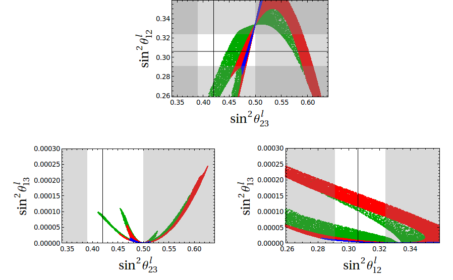
Figure 1: Correlations among the lepton mixing angles when two real parameters $\xi$ and $t_{D}$ are varied randomly. The points with different colors correspond to $|t_{D}|<1$ (blue), $1\leq|t_{D}|<5$ (red) and $5\leq|t_{D}|<10$ (green). The black lines are the updated central values of $\sin^{2}\theta_{12}^{l}$ and $\sin^{2}\theta_{23}^{l}$ obtained by the global fits on neutrino oscillation data fogli . The unshaded and the shaded regions correspond to $1\sigma$ and $3\sigma$ bounds respectively.

It is seen from Fig. (1) that the perturbation induced by type-I term cannot generate considerable deviation in the reactor angle if the other two mixing angles are to remain within their 3$\sigma$ range. In particular, requiring that $\sin^{2}\theta_{12}^{l}$ remains within the 3$\sigma$ range puts an upper bound $\sin^{2}\theta_{13}^{l}\leq 0.0002$ which does not agree with the latest results from T2K and MINOS showing that a small perturbation from type-I term cannot be consistent with data when the type-II term displays exact TBM.

IV.2 Perturbation from the charged lepton mixing

A different class of perturbation to TBM arise when $U_{l}$ deviates from its $Z_{2}\times Z_{2}$ symmetric form given in Eq. (11). In this case, the neutrino mass matrix has TBM structure but the charged lepton mixing leads to departure from it. This case has been considered in the general context leptonic as well as in $SO(10)$ context ab . Within our approach, we can systematically look at the perturbations which change the values of any one or more angles from the TBM value. For example, we can choose $U_{l}$ as given in Eq. (18) and look at the quality of fits in this case compared to the exact TBM solution. This choice (corresponding to $\mu$-$\tau$ symmetry) leaves $\theta_{23}^{l}$ and $\theta_{13}^{l}$ unchanged but perturbs $\theta_{12}^{l}$. Alternative possibility is to simultaneously perturb all three mixing angles and look at the quality of fit compared to the exact TBM case. We follow this approach. For this we choose $U_{l}$ to be a general unitary matrix and go back to the analysis in Section III-A. There, we have fitted the solar and the atmospheric mixing angles to their low energy values given in Table 1. Here, we modify the definition of $\chi^{2}$ and pin down a specific value $o_{i}$ of the mixing angles $p_{i}$ by adding a term

$$\chi^{2}_{lm}=\sum_{i}\left(\frac{p_{i}-o_{i}}{0.01o_{i}}\right)^{2}~{}$$ (26)

to $\chi^{2}_{q}$ that contains all the observables of the quark sector. Sum in Eq. (26) runs over the three lepton mixing angles. The $\chi^{2}=\chi^{2}_{q}+\chi^{2}_{lm}$ is then numerically minimized to fit the 13 observables determined in terms of 12 real parameters as mentioned in Section III-A. Artificially introduced small errors in Eq. (26) fix the value $o_{i}$ for $p_{i}$ at the minimum of the $\chi^{2}$. We then look at the quantity

$$\bar{\chi}^{2}_{min}\equiv\chi^{2}|_{min}-\chi^{2}_{lm}|_{min}$$ (27)

which represents the fit to the quark spectrum when the lepton mixing angles $p_{i}$ are pinned down to values $o_{i}$. We repeat such analysis by randomly varying $o_{i}$ within the allowed 3$\sigma$ ranges of lepton mixing angles fogli . The results are displayed in Fig. (2).

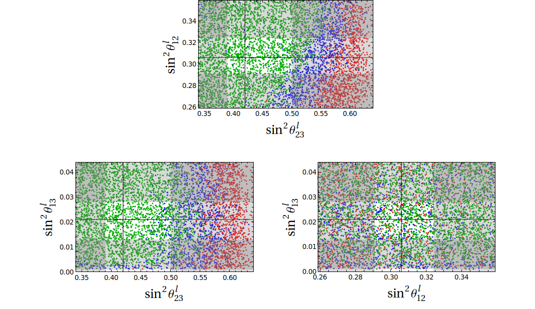
Figure 2: Correlations among the lepton mixing angles in case of the most general charged lepton mixing matrix $U_{l}$. The points with different colors correspond to $\bar{\chi}^{2}_{min}<1$ (green), $1\leq\bar{\chi}^{2}_{min}<4$ (blue) and $\bar{\chi}^{2}_{min}\geq 4$ (red). The black lines are the updated central values of $\sin^{2}\theta_{12}^{l}$ and $\sin^{2}\theta_{23}^{l}$ obtained by the global fits on neutrino oscillation data fogli . The unshaded and the shaded regions correspond to $1\sigma$ and $3\sigma$ bounds respectively.

We plot the correlations among the lepton mixing angles and show the corresponding values of $\bar{\chi}^{2}_{min}$ in three different regions. The points corresponding to $\bar{\chi}^{2}_{min}<1$ (green) represent very good fit in which all the observables are fitted within 1$\sigma$. The obtained fit shown by the points corresponding to $1\leq\bar{\chi}^{2}_{min}<4$ (blue) is not as good as the previous one but it is statistically acceptable. The points for $\bar{\chi}^{2}_{min}>4$ (red) represent poor fit and can be ruled out at 95% confidence level. Fig. (2) shows definite correlations between $\theta_{23}^{l}$ and $\theta_{12}^{l}$. It is seen that the region $\bar{\chi}^{2}_{min}<4$ falls largely below $\sin^{2}\theta_{23}^{l}=0.58$ for $\sin^{2}\theta_{12}^{l}=0.306$. It is also seen from the figure that the entire range $0.001\leq\sin^{2}\theta_{13}^{l}\leq 0.044$ is consistent with statistically acceptable fits to fermion spectrum. This is to be contrasted with the previous case where perturbation from type-I seesaw term led to an upper bound. The bounds obtained numerically allows us to clearly distinguish the case of the exact TBM at $M_{GUT}$ in comparison to the one in which the charged leptons lead to departures from the tri-bimaximality.

V Summary

The presently available information on the leptonic mixing may be described by a TBM structure for ${\cal M}_{\nu f}~{}$combined with appropriate perturbations generating relatively large $\theta_{13}^{l}$. We have analyzed the viability of this scenario in a larger context of the grand unified $SO(10)$ theory taking a specific model as an example. The TBM structure for the neutrino mass matrix is a matter of choice of the basis ab . Thus the existence of TBM is linked to the structure of the charged lepton mixing matrix $U_{l}$ in this basis. All the related studies in this context leptonic ; ab assume that $U_{l}$ deviates slightly from identity and discuss the breaking of the TBM pattern through such $U_{l}$. We have shown that it is possible to construct a class of non-trivial $U_{l}$ quite different from identity which preserve the TBM structure of $M_{\nu}$ when transformed to the flavour basis. Identification of such non-trivial $U_{l}$ becomes crucial in the context of $SO(10)$ and allows us to obtain a viable fit to fermion spectrum keeping TBM intact. The quality of fit obtained in this case is excellent as shown in Table 2 and differs only marginally from a general situation without imposing the TBM structure at the outset.

The existence of TBM at the GUT scale may be inferred by considering its breaking which can arise in the model and the reactor mixing angle is a good pointer to this. The quantum corrections are known rg to lead to very small $\theta_{13}^{l}$ for the hierarchical neutrinos. Similarly, corrections coming from type-I seesaw term imply an upper bound, $\sin^{2}\theta_{13}^{l}\leq 0.0002$ as discussed in Section IV-B. These two cases can be ruled out by relatively large value of $\theta_{13}^{l}$ as indicated by the observations from T2K and MINOS. These cases are in sharp contrast to a situation in which one does not impose the TBM at $M_{GUT}$ and determined $U_{l}$ from a detailed fits to fermion masses. We have analyzed this scenario using the results from the latest fogli global fits to neutrino oscillation data. It is found that the entire range $0.001\leq\sin^{2}\theta_{13}^{l}\leq 0.044$ is consistent with the detailed description of all the fermion masses and mixing angles.

Acknowledgements
Computations needed for the results reported in this work were done using the PRL 3TFLOP cluster at Physical Research Laboratory, Ahmedabad. ASJ thanks the Department of Science and Technology, Government of India for support under the J. C. Bose National Fellowship programme, grant no. SR/S2/JCB-31/2010.

VI Appendix

In this Appendix, we show the parameter values for each of the two cases (A) and (B1) in Table 2. The given values of the matrices $H$, $F$, $G$ and parameters $r,~{}s,~{}t_{l}$ and $t_{u}$ are at the minimum of $\chi^{2}$ and obtained from our fitting procedure. All the physical mass matrices can be constructed from the given numbers using the $SO(10)$ relations in Eq. (III).

Case A: The most general $V_{l}$

The parameter values corresponding to the best fit solution shown in column A in Table 2 are the following.

$$H = \left(\begin{array}[]{ccc}0.00286198&0.00178975&-0.0399313\\ 0.00178975&0.0196685&0.00741417\\ -0.0399313&0.00741417&1.10192\end{array}\right){\rm GeV}$$ (31)

$$F = \left(\begin{array}[]{ccc}-0.00235758&-0.0053869&-0.0053869\\ -0.0053869&-0.0394516&0.0317071\\ -0.0053869&0.0317071&-0.0394516\end{array}\right){\rm GeV}$$ (35)

$$G = \left(\begin{array}[]{ccc}0&-0.00144676&-0.00442083\\ 0.00144676&0&-0.0183052\\ 0.00442083&0.0183052&0\end{array}\right){\rm GeV}$$ (39)

$$(r,~{}s,~{}t_{u},~{}t_{l}) = (76.2076,~{}0.54487,~{}-0.870094,~{}-14.5065)$$

Case B: Exact TBM lepton mixing ($V_{l}=U_{l}$)

The parameter values corresponding to the best fit solution shown in column B1 in Table 2 are the following.

$$H = \left(\begin{array}[]{ccc}0.00111546&0.000428794&-0.020097\\ 0.000428794&0.0188148&0.0639684\\ -0.020097&0.0639684&1.17731\end{array}\right){\rm GeV}$$ (43)

$$F = \left(\begin{array}[]{ccc}-0.0016484&-0.00375321&-0.00375321\\ -0.00375321&-0.0276748&0.0222732\\ -0.00375321&0.0222732&-0.0276748\end{array}\right){\rm GeV}$$ (47)

$$G = \left(\begin{array}[]{ccc}0&-0.00278749&-0.0378996\\ 0.00278749&0&-0.0820076\\ 0.0378996&0.0820076&0\end{array}\right){\rm GeV}$$ (51)

$$(r,~{}s,~{}t_{u},~{}t_{l}) = (70.5742,~{}0.526782,~{}0.551405,~{}2.15986)$$

References

- (1) P. F. Harrison, D. H. Perkins and W. G. Scott, Phys. Lett. B 458, 79 (1999) [arXiv:hep-ph/9904297]; P. F. Harrison, D. H. Perkins and W. G. Scott, Phys. Lett. B 530, 167 (2002) [arXiv:hep-ph/0202074]; Z. -z. Xing, Phys. Lett. B533, 85-93 (2002) [hep-ph/0204049].
- (2) G. Altarelli and F. Feruglio, Rev. Mod. Phys. 82, 2701 (2010) [arXiv:1002.0211 [hep-ph]]; A. Y. .Smirnov, [arXiv:1103.3461 [hep-ph]].
- (3) G. L. Fogli, E. Lisi, A. Marrone, A. Palazzo, A. M. Rotunno, [arXiv:1106.6028 [hep-ph]].
- (4) T. Schwetz, M. Tortola, J. W. F. Valle, [arXiv:1108.1376 [hep-ph]].
- (5) K. Abe et al. [T2K Collaboration], Phys. Rev. Lett. 107, 041801 (2011) [arXiv:1106.2822 [hep-ex]].
- (6) P. Adamson et al. [ MINOS Collaboration ], [arXiv:1108.0015 [hep-ex]].
- (7) X. G. He and A. Zee, arXiv:1106.4359 [hep-ph]; S. Morisi, K. M. Patel and E. Peinado, arXiv:1107.0696 [hep-ph]; R. d. A. Toorop, F. Feruglio and C. Hagedorn, arXiv:1107.3486 [hep-ph].
- (8) P. S. Bhupal Dev, R. N. Mohapatra and M. Severson, arXiv:1107.2378 [hep-ph].
- (9) F. Bazzocchi, M. Frigerio, S. Morisi, Phys. Rev. D78 (2008) 116018. [arXiv:0809.3573 [hep-ph]]; F. Bazzocchi, S. Morisi, M. Picariello, E. Torrente-Lujan, J. Phys. G G36 (2009) 015002. [arXiv:0802.1693 [hep-ph]].
- (10) C. S. Lam, Phys. Rev. Lett. 101 (2008) 121602. [arXiv:0804.2622 [hep-ph]]; C. S. Lam, Phys. Rev. D78 (2008) 073015. [arXiv:0809.1185 [hep-ph]].
- (11) G. Altarelli and G. Blankenburg, JHEP 1103, 133 (2011) [arXiv:1012.2697 [hep-ph]].
- (12) B. Dutta, Y. Mimura and R. N. Mohapatra, Phys. Lett. B 603, 35 (2004) [arXiv:hep-ph/0406262].
- (13) W. Grimus and H. Kuhbock, Eur. Phys. J. C 51, 721 (2007) [arXiv:hep-ph/0612132].
- (14) A. S. Joshipura, B. P. Kodrani and K. M. Patel, Phys. Rev. D 79, 115017 (2009) [arXiv:0903.2161 [hep-ph]].
- (15) A. S. Joshipura and K. M. Patel, Phys. Rev. D 83, 095002 (2011) [arXiv:1102.5148 [hep-ph]].
- (16) B. Bajc, G. Senjanovic and F. Vissani, Phys. Rev. Lett. 90, 051802 (2003) [arXiv:hep-ph/0210207]; H.S. Goh, R.N. Mohapatra, S.P. Ng, Phys. Lett. B 570, 215 (2003) [arXiv:hep-ph/0303055]; H.S. Goh, R.N. Mohapatra, S.P. Ng, Phys. Rev. D 68, 115008 (2003) [arXiv:hep-ph/0308197]; C. S. Aulakh and S. K. Garg, Nucl. Phys. B 757, 47 (2006) [arXiv:hep-ph/0512224]; B. Bajc, A. Melfo, G. Senjanovic and F. Vissani, Phys. Lett. B 634, 272 (2006) [arXiv:hep-ph/0511352]; B. Bajc, I. Dorsner and M. Nemevsek, JHEP 0811, 007 (2008) [arXiv:0809.1069 [hep-ph]]; C. S. Aulakh, B. Bajc, A. Melfo, G. Senjanovic and F. Vissani, Phys. Lett. B 588, 196 (2004) [arXiv:hep-ph/0306242]; K.S. Babu, C. Macesanu, Phys. Rev. D 72, 115003 (2005) [arXiv:hep-ph/0505200]; B. Bajc, A. Melfo, G. Senjanovic and F. Vissani, Phys. Rev. D 70, 035007 (2004) [arXiv:hep-ph/0402122]; S. Bertolini, T. Schwetz and M. Malinsky, Phys. Rev. D 73, 115012 (2006) [arXiv:hep-ph/0605006].
- (17) C. S. Aulakh, Phys. Lett. B 661, 196 (2008) [arXiv:0710.3945 [hep-ph]]; C. S. Aulakh and S. K. Garg, arXiv:0807.0917 [hep-ph]; N. Oshimo, Phys. Rev. D 66, 095010 (2002) [arXiv:hep-ph/0206239]; N. Oshimo, Nucl. Phys. B 668, 258 (2003) [arXiv:hep-ph/0305166]; B. Dutta, Y. Mimura and R. N. Mohapatra, Phys. Rev. Lett. 94, 091804 (2005) [arXiv:hep-ph/0412105]; B. Dutta, Y. Mimura and R. N. Mohapatra, Phys. Rev. D 72, 075009 (2005) [arXiv:hep-ph/0507319]; W. M. Yang and Z. G. Wang, Nucl. Phys. B 707, 87 (2005) [arXiv:hep-ph/0406221]; S. Bertolini and M. Malinsky, Phys. Rev. D 72, 055021 (2005) [arXiv:hep-ph/0504241]; C. S. Aulakh, arXiv:hep-ph/0602132; C. S. Aulakh and S. K. Garg, arXiv:hep-ph/0612021.
- (18) H. S. Goh, R. N. Mohapatra and S. Nasri, Phys. Rev. D 70, 075022 (2004) [arXiv:hep-ph/0408139].
- (19) A. Melfo, A. Ramirez and G. Senjanovic, Phys. Rev. D 82, 075014 (2010) [arXiv:1005.0834 [hep-ph]].
- (20) C. R. Das and M. K. Parida, Eur. Phys. J. C 20, 121 (2001) [arXiv:hep-ph/0010004].
- (21) T. Araki, C. -Q. Geng, Z. -z. Xing, [arXiv:1012.2970 [hep-ph]]; A. Dighe, S. Goswami, W. Rodejohann, Phys. Rev. D75 (2007) 073023. [hep-ph/0612328].
- (22) F. Plentinger, W. Rodejohann, Phys. Lett. B625 (2005) 264-276. [hep-ph/0507143]; K. A. Hochmuth, S. T. Petcov and W. Rodejohann, Phys. Lett. B 654, 177 (2007) [arXiv:0706.2975 [hep-ph]]; S. F. King, Phys. Lett. B 659, 244 (2008) [arXiv:0710.0530 [hep-ph]]; S. Boudjemaa and S. F. King, Phys. Rev. D 79, 033001 (2009) [arXiv:0808.2782 [hep-ph]]; C. H. Albright and W. Rodejohann, Eur. Phys. J. C 62, 599 (2009) [arXiv:0812.0436 [hep-ph]]; Y. Shimizu and R. Takahashi, Europhys. Lett. 93, 61001 (2011) [arXiv:1009.5504 [hep-ph]]; S. F. King, JHEP 1101, 115 (2011) [arXiv:1011.6167 [hep-ph]]; D. Meloni, F. Plentinger and W. Winter, Phys. Lett. B 699, 354 (2011) [arXiv:1012.1618 [hep-ph]]; A. Adulpravitchai, K. Kojima and R. Takahashi, JHEP 1102, 086 (2011) [arXiv:1012.1760 [hep-ph]]; Y. H. Ahn, H. Y. Cheng and S. Oh, Phys. Rev. D 83, 076012 (2011) [arXiv:1102.0879 [hep-ph]].