Modeling supernova remnants: effects of diffusive cosmic-ray acceleration on the evolution, application to observations

We present numerical models for supernova remnant evolution, using a new version of the hydrodynamical code SUPREMNA. We added cosmic ray diffusion equation to the code scheme, employing two-fluid approximation. We investigate the dynamics of the simulated supernova remnants with different values of cosmic ray acceleration efficiency and diffusion coefficient. We compare the numerical models with observational data of Tycho’s and SN1006 supernova remnants. We find models which reproduce the observed locations of the blast wave, contact discontinuity, and reverse shock for the both remnants, thus allowing us to estimate the contribution of cosmic ray particles into total pressure and cosmic-ray energy losses in these supernova remnants. We derive that the energy losses due to cosmic rays escape in Tycho’s supernova remnant are 10-20% of the kinetic energy flux and 20-50% in SN1006.

1 Introduction

Clear evidence for effective acceleration of cosmic-ray (CR) particles in young supernova remnants (SNR) stems from TeV observations of the Galactic sources by HESS (Aharonian et al. 2005, 2006), CANGAROO-II (Katagiri et al. 2005), MAGIC (Albert et al. 2007), SHALON (Sinitsyna et al. 2009), VERITAS (Acciari et al. 2009, 2010). In addition, discoveries of non-thermal X-ray emission from SNRs (see a review by Reynolds 2008) point to the presence of electrons accelerated to TeV energies in supernova remnants (SNR).

In the last decades a number of numerical methods which account for CR acceleration in simulations of supernova remnants were developed. An extensive review of some of these techniques can be found in Malkov & O’C Drury (2001) and Caprioli et al. (2010). Nearby Galactic SNRs provide an excellent opportunity to test these models and to study the efficiency of CR acceleration processes. For example, the proximity of the blast wave (BW) to contact discontinuity (CD) in Tycho SNR measured by Warren et al. (2005) is inconsistent with adiabatic hydrodynamic models of SNR evolution, and can be explained only if cosmic-ray acceleration of the particles occurs at the forward shock. The similar evidence was presented for SN1006 supernova remnant by Cassam-Chenaï et al. (2008) and Miceli et al. (2009).

Both these objects were already used in testing of the numerical and analytical models (e.g. Ellison 2001, Ellison et al. 2007, Völk et al. 2008) of CR acceleration in SNRs. 2D simulations of Tycho’s SNR evolution and investigation of Rayleigh-Taylor instability development with the gas adiabatic index values down to $\gamma=1.1$ were performed by Wang (2010). 3D hydrodynamical modeling of Tycho was conducted by Ferrand et al. (2010).

The effects of the shock modification by cosmic rays in Kepler SNR were studied by Decourchelle et al. (2000), who modeled the X-ray spectra using a non-linear non-equilibrium ionization method. A more detailed study of the acceleration effects on the thermal emission from the shocked supernova ejecta was conducted by Patnaude et al. (2010).

In this study we present hydrodynamical (HD) simulations of supernova remnant evolution with the account for diffusive cosmic-ray acceleration. We introduced a CR diffusion equation into the numerical code supremna, developed by Sorokina et al. (2004), Kosenko (2006). This code calculates the evolution of a supernova remnant assuming spherical symmetry and taking into account time-dependent ionization and thermal conduction. To include the effects of CR acceleration into the scheme, we apply a two-fluid approximation, i.e. we introduce a CR diffusion equation into the system of hydrodynamical equations.

Employing this renewed package we have created sets of hydrodynamical models with different values of CR-related parameters. We compare the results of our simulations with the observations of Tycho’s and SN1006 supernova remnants.

The paper is structured as follows. In Section 2 we describe the basic equations we use for the simulations, in Section 3 we show the results of modeling. We compare our models with the observations in the Section 4. We summarize the results in Section 5, discuss them in Section 6 and conclude by Section 7.

2 Basic equations and method

2.1 Code description

For modeling the evolution of supernova remnants, we employ the hydrodynamical code supremna, which was introduced by Sorokina et al. (2004). The method accounts for electron thermal conduction and includes self-consistent calculations of time-dependent ionization processes. The electron and ion temperature equilibration processes are parametrized.

The code uses an implicit Lagrangean formulation for one dimensional spherical-symmetrical geometry. The hydrodynamical evolution of the remnant is coupled with the system of kinetic equations of ionization balance to calculate self-consistently non-equillibrium ionization state of the shocked plasma. Ion and electron temperatures are treated separately taking into account electron thermal conduction (see Appendix A).

To describe the effects of collisionless energy exchange, Sorokina et al. (2004) introduced a parameter $q_{i}$ ($0<q_{i}<1$) which specifies a fraction of artificial viscosity $Q$, added to the pressure of ions in the equations (10), (12) and plays a role of a source term (the details are presented in the Appendix). If only the collisional exchange is taken into account, then $q_{i}=(1.0-m_{e}/m_{p})$ and the standard system of equations with the heating of just ions at the front is being solved.

The artificial viscosity (Richtmyer & Morton 1967) term is defined as follows

$$Q=\left\{\begin{array}[]{cc}A_{q}\rho(\Delta u)^{2}&\mathrm{if}\;(\Delta u)<0\\ 0&\mathrm{otherwise},\\ \end{array}\right.$$ (1)

with dimensionless parameter $A_{q}=2$ and $\Delta u$ — velocity difference at neighboring mesh points.

2.2 Cosmic-ray diffusion equation

In order to tailor the scheme for simulations of SNRs we need to take into account cosmic-ray (CR) diffusion. We used two-fluid approximation (e.g. Kang & Jones 1990, Ko 1995, Malkov & O’C Drury 2001, Blasi 2002, 2004, Wagner et al. 2006, Zirakashvili & Aharonian 2010) and introduced additional CR diffusion equation into the (8)-(12) set.

The one-dimensional CR diffusion equation in the Eulerian frame for the plane-parallel case reads

$${\partial E_{\mathrm{CR}}\over\partial t}+{\partial(uE_{\mathrm{CR}})\over\partial r}-{\partial\over\partial r}\left(\kappa_{\mathrm{CR}}{\partial E_{\mathrm{CR}}\over\partial r}\right)+P_{\mathrm{CR}}{\partial u\over\partial r}=\Theta,$$ (2)

where $P_{\mathrm{CR}}=(\gamma_{\mathrm{CR}}-1)E_{\mathrm{CR}}$ is CR pressure, $E_{\mathrm{CR}}$ — CR energy density, $\Theta$ is an external source of CR energy injection, $\kappa_{\mathrm{CR}}$ — diffusion coefficient. We assume equation of state for CR matter with the fixed adiabatic exponent of $\gamma_{\mathrm{CR}}=4/3$,

We generate relativistic particles pressure $P_{\mathrm{CR}}$ from the artificial viscosity $Q$ term by introducing a parameter $q_{\mathrm{CR}}$, that regulates the injection of CR particles. Thus we define the source term as $\Theta=q_{\mathrm{CR}}Q(\partial u/\partial r)$ (see Appendix B).

Note that a somewhat similar method was used by Zank et al. (1993), where the introduction of a source term into CR diffusion equation was performed via a “thermal leakage” mechanism. Particle distribution function was divided in two parts, those particles that have momentum higher than a certain value $p_{0}$ were treated as CR which propagate according to the CR diffusion equation. Thermal particles are energized due to the adiabatic compression or anomalous heating within a subshock.

In our study we are not concerned with microphysics of the generation and escape of the energetic particles, but more with hydrodynamical consequences of the acceleration.

After transformation of the equation (2) to our adopted Lagrangian frame, we get

$${DE_{\mathrm{CR}}\over Dt}= - (E_{\mathrm{CR}}+P_{\mathrm{CR}})\,4\pi\rho{\partial(r^{2}u)\over\partial m}$$ (3)

$$+ 4\pi\rho{\partial\over\partial m}\left(r^{2}\,F_{\mathrm{CR}}\right)-4\pi\rho{\partial(r^{2}u)\over\partial m}q_{\mathrm{CR}}Q,$$

where $DE_{\mathrm{CR}}/Dt=\partial E_{\mathrm{CR}}/\partial t+4\pi r^{2}u\rho(\partial E_{\mathrm{CR}}/\partial m)$.

We treat cosmic-ray flux $F_{\mathrm{CR}}$ in the same manner as it is done for thermal electron conduction in Sorokina et al. (2004).

$$F_{\mathrm{CR}}={-\kappa_{\mathrm{CR}}\nabla E_{\mathrm{CR}}\over{1+\left|\kappa_{\mathrm{CR}}\nabla E_{\mathrm{CR}}\right|/F_{\mathrm{sat\;CR}}}},$$ (4)

where $F_{\mathrm{sat\;CR}}=cP_{\mathrm{CR}}/2$ ($c$ — speed of light) is saturated value of the cosmic-ray flux (the Eddington approximation). At this stage we assume a constant diffusion coefficient $\kappa_{\mathrm{CR}}$, as we do not have information on the spectrum of cosmic rays.

In reality the diffusion will depend on particle energy. In that case the diffusion coefficient used by us should be regarded as an pressure weighted mean value. Moreover, according to non-linear cosmic ray acceleration theory, efficient acceleration leads to hard spectra, in which case most of the energy, and hence pressure, is contained by the particles with the highest energies. If the maximum energy is around $10^{15}$ eV we expect a typical diffusion coefficient, under the assumption of Bohm-diffusion, of $\kappa_{\mathrm{CR}}=1/3r_{g}c=3\times 10^{26}(B/100\,\mu\mathrm{G})^{-1}(E/10^{15}\,\mathrm{eV})\;\mathrm{cm}^{2}\mathrm{s}^{-1}$ ($r_{g}$ — gyroradius, $B$ — magnetic field, $E$ — energy of the particle). The largest role of the diffusion coefficient for our calculations is in the role of CR escape, as it drains energy from the plasma.

And finally, we alter the equation (10) by adding a component of relativistic particle pressure $P_{\mathrm{CR}}$ in such a way that

$${\partial u\over\partial t}=-4\pi r^{2}\,{\partial(P_{e}+P_{i}+P_{\mathrm{CR}})\over\partial m}-{Gm\over r^{2}}.$$ (5)

The entire system of equations (8), (5), (11), (12) and (3) describes the system, where electrons, ions and cosmic-ray components are treated independently. The contributions to the pressure of these three components are governed by two free parameters $q_{\mathrm{i}}$ and $q_{\mathrm{CR}}$.

3 Numerical models

We created a library of numerical models with various sets of parameters $q_{\mathrm{CR}}$ and $\kappa_{\mathrm{CR}}$. In the simulations we used a delayed-detonation thermonuclear explosion model with $E=1.4\times 10^{51}$ erg (Woosley et al. 2007), initially the CR pressure is $P^{0}_{\mathrm{CR}}=10^{-10}P_{i}$, and the temperature of the homogeneous ambient medium is $T_{0}=10^{4}$ K. Using the artificial viscosity source term, we turn on CR generation only at the forward shock.

We considered two sets of models of supernova remnants. Parameters for one set (Tycho’s case) were taken similar to Tycho’s SNR: the remnant is surrounded with homogeneous circumstellar matter of density $\rho_{0}=10^{-24}\;\mathrm{g\,cm}^{-3}$ and the age of the system is 440 years. Note, that there are indications, that the real ambient density in Tycho vicinity is lower. For example, Katsuda et al. (2010) from proper motion measurements found that $n_{0}\lesssim 0.2\;\mathrm{cm}^{-3}$, thus $\rho_{0}\lesssim 0.4\times 10^{-24}\;\mathrm{g\,cm}^{-3}$. Nevertheless, taking into account that we consider over-energetic initial explosion and that radius of the remnant $R\propto(E/\rho_{0})^{1/5}$ is a weak function of ambient density, we assume that our input parameters match Tycho’s SNR.

Examples of hydrodynamical profiles of a few of these models are presented in Fig. 1. Top row shows the simulation with $q_{\mathrm{CR}}=0.0$, middle row — $q_{\mathrm{CR}}=0.7$, $\kappa_{\mathrm{CR}}=10^{25}\,\mathrm{cm}^{2}\mathrm{s}^{-1}$; bottom row — $q_{\mathrm{CR}}=0.99$, $\kappa_{\mathrm{CR}}=10^{26}\,\mathrm{cm}^{2}\mathrm{s}^{-1}$. Left panels: density (black solid, scale at the left-hand side), ion pressure (blue dash-dotted, scale at the right-hand side), CR pressure (blue dashed, scale at the right-hand side). Right panels: solid line shows velocity profile (scale at the left-hand side), dashed line — electron temperature profiles, dashed-dotted line — ion temperature profiles (scale at the right-hand side).

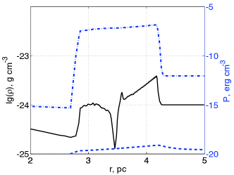
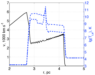
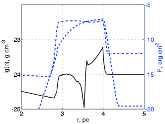
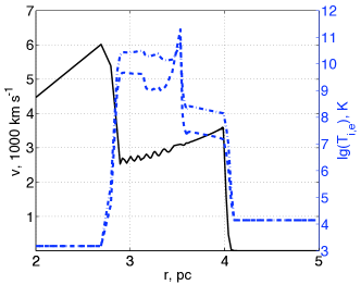
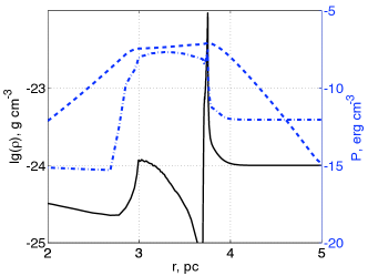
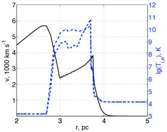
Figure 1: HD profiles for the SNR models at $t=440$ years with $\rho_{\mathrm{CSM}}=10^{-24}\,\mathrm{g\,cm}^{-3}$. Top row shows the simulation with $q_{\mathrm{CR}}=0.0$, middle row — $q_{\mathrm{CR}}=0.7$, $\kappa_{\mathrm{CR}}=10^{25}\;\mathrm{cm}^{2}\mathrm{s}^{-1}$; bottom row — $q_{\mathrm{CR}}=0.99$, $\kappa_{\mathrm{CR}}=10^{26}\;\mathrm{cm}^{2}\mathrm{s}^{-1}$. Left panels: density (black solid line, scale at the left-hand side), ion pressure (blue dash-dotted line, scale at the right-hand side), CR pressure (blue dashed line, scale at the right-hand side). Right panels: velocity profile (black solid line, scale at the left-hand side), electron temperature profiles (blue dashed line, scale at the right-hand side), ion temperature profiles (dashed-dotted line, scale at the right-hand side).

Physical parameters of another set (SN1006 case) were chosen to match the remnant of SN1006 conditions: an ambient homogeneous circumstellar matter of density $\rho_{0}=4\times 10^{-26}\;\mathrm{g\,cm}^{-3}$ and the age of 1000 years. Hydrodynamical profiles of a few of these models are presented in Fig. 2.

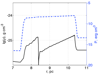
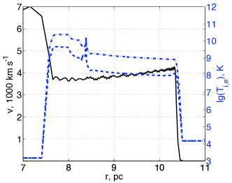
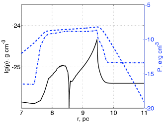
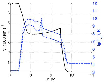
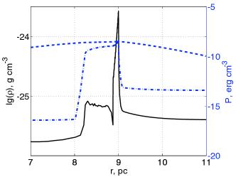
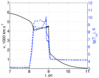
Figure 2: HD profiles for the SNR models at $t=1000$ years with $\rho_{\mathrm{CSM}}=4\times 10^{-26}\,\mathrm{g\,cm}^{-3}$. Top row shows the simulation with $q_{\mathrm{CR}}=0.0$, middle row — $q_{\mathrm{CR}}=0.7$, $\kappa_{\mathrm{CR}}=10^{25}\;\mathrm{cm}^{2}\mathrm{s}^{-1}$; bottom row — $q_{\mathrm{CR}}=0.99$, $\kappa_{\mathrm{CR}}=10^{26}\;\mathrm{cm}^{2}\mathrm{s}^{-1}$. Left panels: density (black solid line, scale at the left-hand side), ion pressure (blue dash-dotted line, scale at the right-hand side), CR pressure (blue dashed line, scale at the right-hand side). Right panels: velocity profile (black solid line, scale at the left-hand side), electron temperature profiles (blue dashed line, scale at the right-hand side), ion temperature profiles (dashed-dotted line, scale at the right-hand side).

The numerical models were verified to satisfy the Rankine-Hugoniot condition, derived for the system with energy losses (e.g. Malkov & O’C Drury 2001, Bykov et al. 2008, Vink et al. 2010). Namely the following relation was checked

$$\chi={\gamma+1\over\gamma-\sqrt{1+2(\gamma^{2}-1)Q_{\mathrm{esc}}/(\rho_{0}v_{\mathrm{S}}^{3})}}$$ (6)

where $\chi=\rho_{\mathrm{max}}/\rho_{0}$ is the compression ratio behind the shock, $\gamma$ — adiabatic index, $Q_{\mathrm{esc}}$ — energy lost by the system, $v_{\mathrm{S}}$ — blast wave speed. We rewrite the energy losses term from the energy flux conservation law (e.g. formula (12) in Vink et al. 2010) via a dimensionless parameter as

$$\epsilon_{\mathrm{esc}}=2Q_{\mathrm{esc}}/(\rho_{0}v_{\mathrm{S}}^{3})=1-{1\over\chi^{2}}-{E+P\over\rho v_{\mathrm{S}}^{2}/2}$$ (7)

where $E,P,\rho$ are total energy density, pressure and matter density behind the shock.

The top panel of Fig. 3 shows the relation (6) for $\gamma=5/3$ — solid line and $\gamma=4/3$ — dashed line. Data from the numerical models are presented with colored circles. Hue reflects the efficiency of CR acceleration, so that red point correspond to the models with $q_{\mathrm{CR}}=0.1$ and cyan — to the models with $q_{\mathrm{CR}}=0.99$.

The bottom panel of Fig. 3 shows evolution of the compression ratio and ratio of the contact discontinuity (CD) to blast wave (BW) radii. The profiles are created from the Tycho’s case models with $\rho_{0}=10^{-24}\,\mathrm{g\,cm}^{-3}$. Dashed lines show the simulation with $q_{\mathrm{CR}}=0.7$, solid lines — $q_{\mathrm{CR}}=0.9$. Different colors correspond to different values of $\kappa_{\mathrm{CR}}$ (see legend). The curves are compared to those from Völk et al. (2008). We see that $\chi$ profiles differ from the curves presented for Tycho’s SNR in Völk et al. (Fig. 1 in 2008). In our approach the compression ratio is an increasing function of time, whereas in Völk et al. (2008) $\chi$ decreases with time. Radii ratio in our cases also does not follow exactly the same trend as in Völk et al. (2008).

This divergence in the results can be explained by the magnetic field behind the shock. Völk et al. (2005) show that on average the downstream magnetic field pressure $B^{2}/(8\pi)$ is proportional to preshock gas ram pressure $\rho_{0}v_{\mathrm{S}}^{2}$. The ram pressure and the magnetic field dilutes as the remnant expands, thus the acceleration decreases. In our models, the acceleration efficiency depends only on the ram pressure (Eq. 1) and does not take into account the vanishing magnetic field. Thus with a constant $q_{\mathrm{CR}}$ parameter, we somewhat underestimate the efficiency of the CR acceleration at the earlier times of the evolution and we overestimate it at the later times.

Note, that for the simulation with efficient acceleration $q_{\mathrm{CR}}=0.9$ and with diffusion coefficient $\kappa_{\mathrm{CR}}=10^{27}\;\mathrm{cm}^{2}\mathrm{s}^{-1}$ (solid magenta line) at the age of more than 1000 years a density spike starts to form. Structure of such a spike is illustrated in the bottom rows of Fig. 1 and Fig. 2. Similar spikes are also present in the CR dominated shocks in simulations of Wagner et al. (2009). Nevertheless, this type of structure is produced only at the extreme values of CR parameters and is unlikely to be realized in nature.

The CR precursor can be traced in the hydrodynamical profiles, presented in Fig. 1 and Fig. 2, but the precursor region in front of the blast wave is thin ($\sim 10^{17}\;\mathrm{cm}$) and cannot be accurately resolved.

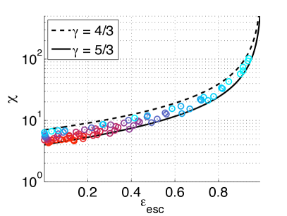
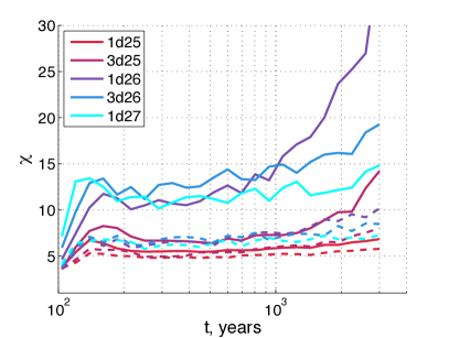
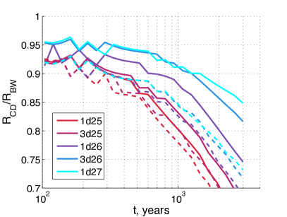
Figure 3: Top panel: Rankine-Hugoniot relation (6) and data points from all the numerical models. Hue reflects the efficiency of CR acceleration. Bottom row: left panel shows evolution of compression ration $\chi$, right panel shows evolution of contact discontinuity to blast wave radii ratio, $\rho_{0}=10^{-24}\,\mathrm{g\,cm}^{-3}$. Dashed lines show models with $q_{\mathrm{CR}}=0.7$, solid lines — $q_{\mathrm{CR}}=0.9$. Different colors indicate different values of the diffusion coefficient (see legend, where $\kappa_{\mathrm{CR}}$ values are given in units of $\;\mathrm{cm}^{2}\mathrm{s}^{-1}$).

4 Comparison with the Galactic SNRs

There is an evidence that the shocks of Tycho (e.g. Warren et al. 2005) and SN1006 (Cassam-Chenaï et al. 2008, Orlando et al. 2008, Miceli et al. 2009) are modified by acceleration and diffusion of CR particles. Thus, we applied our numerical models to these Galactic supernova remnants. Locations of the blast wave (BW), the contact discontinuity (CD) and the reverse shock (RS) measured by Warren et al. (2005) for Tycho’s SNR, were compared with the corresponding values obtained in our simulations.

The right plot of Fig. 4 shows the measured (horizontal strip) radii ratios and also results of the simulations (asterisks). To account for the three-dimentional projection effects and Rayleigh-Taylor (R-T) instabilities, that can produce fingers of ejecta that protrude out toward the BW (Chevalier et al. 1992, Wang & Chevalier 2001) we adopt a correction factor of $1.07$ (Warren et al. 2005, Cassam-Chenaï et al. 2008, Völk et al. 2008, and references therein) to the modeled CD:BW radii ratios. The models that match the observed radii are boldfaced.

We also performed simulations with CR acceleration at the reverse shock with the same injection efficiency $q_{\mathrm{CR}}$ and diffusion coefficient $\kappa_{\mathrm{CR}}$ as at the blast wave. In these models the layer of the shocked supernova ejecta becomes thinner, and the reverse shock approaches too close to the forward shock compared to the data from Tycho’s SNR. Thus, we did not study these scenarios in details.

From an analysis of the data, presented in Fig. 4, we derive that the most plausible models for Tycho are with $q_{\mathrm{CR}}=0.5-0.7$, $\kappa_{\mathrm{CR}}=10^{24}-10^{25}\;\mathrm{cm}^{2}\mathrm{s}^{-1}$. In fact, models with $q_{\mathrm{CR}}=0.3$, $\kappa_{\mathrm{CR}}=10^{26}\;\mathrm{cm}^{2}\mathrm{s}^{-1}$ and $q_{\mathrm{CR}}=0.9$, $\kappa_{\mathrm{CR}}=10^{24}\;\mathrm{cm}^{2}\mathrm{s}^{-1}$ also match the observation. Nevertheless, if we assume that diffusion coefficient $\kappa_{\mathrm{CR}}$ increases with the energy of the CR particles and that the amount of energetic particles increases with the injection efficiency $q_{\mathrm{CR}}$, then we conclude that low efficiency and high diffusion or high efficiency and low diffusion scenarios probably are not realized.

For Tycho, the simulations yield the compression ratio $\chi=4.3-6.8$. These results are in agreement with Cassam-Chenaï et al. (2007) and Völk et al. (2008).

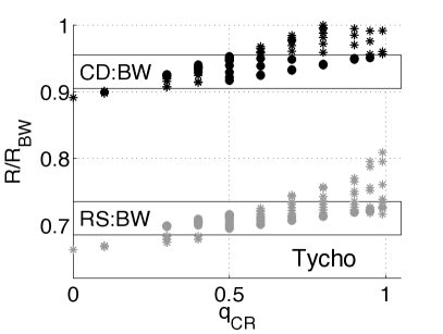
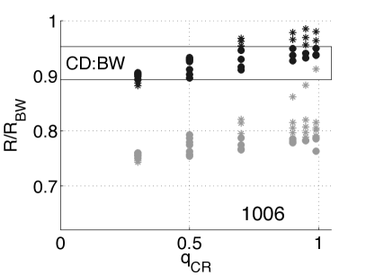
Figure 4: Measured and modeled radii ratios for Tycho’s (left-hand panel) and SN1006 (right-hand panel) SNRs. $R_{\mathrm{CD}}/R_{\mathrm{RW}}$ (black symbols) and $R_{\mathrm{RS}}/R_{\mathrm{RW}}$ (grey symbols). Horizontal bars outline the measured by Warren et al. (2005) and Miceli et al. (2009) values.

The similar comparison of the models to with SN1006 remnant data (Miceli et al. 2009) is presented on the right plot of Fig. 4. From these models we obtain the compression ratio behind the blast wave of the remnant $\chi=4.7-8.3$. All the models with $q_{\mathrm{CR}}=(0.3-0.9)$ match the observational data. Note, that models of SN1006 with constant adiabatic index $\gamma$ (Petruk et al. 2011) could not explain the observed small distance between forward shock and contact discontinuity.

5 Results

We developed a hydro-code to simulate an evolution of a spherically-symmetrical supernova remnants with account for CR acceleration and time-dependent ionization. We created two sets of hydrodynamical models with different values of parameters for CR acceleration efficiency and CR energy losses. The comparison of these models with the measurement of BW:CD:RS radii of the Galactic SNRs suggests the following.

The simulations with $q_{\mathrm{CR}}=(0.4-0.7)$ and $\kappa_{\mathrm{CR}}=(10^{24}-10^{25})\;\mathrm{cm}^{2}\mathrm{s}^{-1}$ match the observed radii ratios of Tycho’s SNR (Fig. 4). This range of values covers the estimate $\kappa_{\mathrm{CR}}=2\times 10^{24}\;\;\mathrm{cm}^{2}\mathrm{s}^{-1}$ found by Wagner et al. (2009) for Tycho and are in agreement with the findings of Parizot et al. (2006) and Eriksen et al. (2011). We derived the compression ratio of $\chi=(4.3-6.8)$, energy losses due to CR diffusion is of $\epsilon_{\mathrm{esc}}=(0.1-0.2)$ and distance to Tycho’s SNR of $3.3$ pc . The distance is in agreement with the results of Hayato et al. (2010) and Tian & Leahy (2011).

For SN1006 remnant we obtained $\chi=(4.7-8.3)$ with losses of $\epsilon_{\mathrm{esc}}=(0.2-0.5)$. We derived the distance to the SN1006 remnant as $2.0$ kpc.

6 Discussion

The observed ratios of SNR reverse shock, contact discontinuity and forward shock radii may depend on a number of yet unknown factors, such as structure of the CSM (potential presupernova wind and density enhancement, see discussion in Kosenko et al. 2010, Xu et al. 2010), CR acceleration and diffusion efficiency. Thus the results, presented in this study do not claim to be exhaustive, but rather describe one of the possible scenarios which explains the observations within the cosmic-ray acceleration paradigm.

In the numerical models considered here, we do not turn on CR acceleration at the reverse shock. Results from the simulations with the same acceleration efficiency ($q_{\mathrm{CR}}$) of the relativistic particles at the reverse shock do not match the observed $R_{\mathrm{RS}}/R_{\mathrm{BW}}$ ratio for Tycho’s SNR. Helder & Vink (2008), Zirakashvili & Aharonian (2010) point out to the possible acceleration of particles by the reverse shock of CasA and SNR RX J1713.7–3946. In addition, numerical simulations of Schure et al. (2010) showed, that the reverse shock can re-accelerate particles, provided that the magnetic field is sufficiently strong. However, our models indicate that for Tycho’s SNR the cosmic rays acceleration at the reverse shock is not as efficient as at the forward shock.

The possible factors which suppress the acceleration at the reverse shock are as follows. The reverse shock velocity in the frame of ejecta is lower in comparison with the blast wave, and acceleration efficiency is probably an increasing function of the shock velocity. Moreover, the initial magnetic field of the progenitor white dwarf is diluted in the remnant by many orders of magnitude. Non-vanishing magnetic field is necessary for the acceleration to take place. Also, low efficiency of CR acceleration at the reverse shock was found for Kepler SNR by Decourchelle et al. (2000).

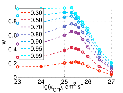
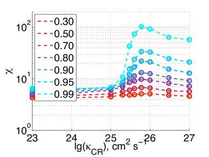
Figure 5: Left panel: CR pressure versus diffusion coefficient. Right panel: compression ratio $\chi$ versus diffusion coefficient $\kappa_{\mathrm{CR}}$ for different values of $q_{\mathrm{CR}}$ (Tycho’s case).

We compared the input and output parameters of the simulation with Rankine-Hugoniot (RH) relations, derived in two-fluid approach for the steady-state situation and a plane-parralel geometry, presented in Vink et al. (2010). On the one hand, the values of $P_{\mathrm{CR}}/P_{\mathrm{tot}}$ measured in the models directly behind the shock cannot be compared to $w$ defined in Vink et al. (2010). The diffusion coefficient $\kappa_{\mathrm{CR}}$ implements the CR energy losses and thus the CR pressure $P_{\mathrm{CR}}$ is a non-monotonic function of $\kappa_{\mathrm{CR}}$ (Fig. 5). Namely, the pressure decreases with $\kappa_{\mathrm{CR}}$ in the regime of efficient acceleration, where $\kappa_{\mathrm{CR}}>3\times 10^{25}\;\mathrm{cm}^{2}\mathrm{s}^{-1}$. This is opposite to the behavior of $w$ defined by Vink et al. (2010). Possible explanation is that spherical symmetrical expansion and inward CR diffusion efficiently dilute the pressure, while in the plane-parallel case described by Vink et al. (2010) these effects are absent.

On the other hand, the parameter $q_{\mathrm{CR}}$ sets the share of the CR pressure taken from the entropy pool created by the shock and in some sense can be attributed to $w$. Fig. 6 shows profiles of compression ration $\epsilon_{\mathrm{esc}}$ (left panel) and CR energy losses $\chi$ (right panel) as a function of $w=P_{\mathrm{CR}}/P_{\mathrm{tot}}$ (Fig. 1 in Vink et al. 2010, for Mach number $M_{0}=500$). In the same panels we plot $\epsilon_{\mathrm{esc}}$ and $\chi$ measured in the models versus the input parameter $q_{\mathrm{CR}}$. The intensity of the data points corresponds to the value of $\kappa_{\mathrm{CR}}$: the lowest value corresponds to the black asterisks, the models with the highest value of $\kappa_{\mathrm{CR}}$ shaded in light gray.

The right-hand plot of Fig. 6 can be explained with the help of the right-hand plot of Fig. 5, where compression ratios versus diffusion coefficient for different acceleration efficiencies $q_{\mathrm{CR}}$ are presented. This plot shows that $\chi$ has a maximum at certain $\kappa_{\mathrm{CR}}$. These maximal values of $\chi$ for different $q_{\mathrm{CR}}$ follow the RH curve, plotted with thick black line in the right plot of Fig. 6. Respectively, the maximum attainable energy losses are skirted by the RH curves, presented in the left panel of Fig. 6.

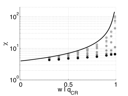
Figure 6: Left panel: escape CR energy versus $w$ and $q_{\mathrm{CR}}$. Right panel: compression ratio $\chi$ versus $w$ and $q_{\mathrm{CR}}$ (Tycho’s case). The Rankine-Hugoniot black curve corresponds for the case of Mach number $M_{0}=500$. Intensity of the data point is invers proportional to the values of diffusion coefficient $\kappa_{\mathrm{CR}}$, i.e. black asterisk correspond to $\kappa_{\mathrm{CR}}=10^{24}\,\;\mathrm{cm}^{2}\mathrm{s}^{-1}$, light grey correspond to $\kappa_{\mathrm{CR}}=10^{27}\,\;\mathrm{cm}^{2}\mathrm{s}^{-1}$.

The parameters $q_{\mathrm{CR}}$ and $\kappa_{\mathrm{CR}}$ are fixed for each model in our method, while in reality they vary with time and location (e.g. Zirakashvili & Aharonian 2010). The effects of the variability of the diffusion coefficient was also discussed extensively by Lagage & Cesarsky (1983), where they point out that $\kappa_{\mathrm{CR}}$ increases away from the shock. Nevertheless, we assume that it is acceptable to use averaged constant values in this approach.

Even though we used two parameters for CR component in our models, in fact, the theory of diffusive CR acceleration assumes that, $q_{\mathrm{CR}}$ and $\kappa_{\mathrm{CR}}$ are not independent. Thus it is possible to incorporate a physical relation between those two in future, reducing the problem to a case with only one free parameter.

At last we note, that in comparison of the models and the observations, we considered also a case with lower R-T correction factor of $1.05$. In this case the models that match the observed radii yield the compression ratio for Tycho’s SNR systematically higher with $\chi=4.6-8.5$, but within the uncertainties of our approach and errors of radii measurements, the final results are not altered considerably.

7 Conclusion

We studied hydrodynamical models of supernova remnants evolution with account of diffusive cosmic-ray acceleration. We applied a two-fluid approach to investigate the effects of acceleration efficiency and energy losses on observable properties on the remnant. We compared the results of our simulations with the measured radii of BW, CD and RS of Tycho’s and SN1006 SNRs.

We analyzed the numerical models and checked that the Rankine-Hugoniot relation for compression ratio and energy losses is met (Fig. 3). This method has a list of shortcomings but it includes all important relevant physical processes and easy to use for fast modeling of supernova remnants and for comparison with observations.

We found that, in order to explain radial properties of Tycho’s SNR, the simulations yield the compression ratio behind the blast wave of $(4.3-6.8)$, energy losses due to cosmic ray particle diffusion of $(0.1-0.2)\rho_{0}v_{\mathrm{S}}^{3}/2$. Distance to Tycho is estimated as $3.3$ pc. For the case of SN1006 remnant, we found $\chi=(4.7-8.3)$ with losses of $(0.2-0.5)\,\rho_{0}v_{\mathrm{S}}^{3}/2$. The distance to the remnant is $2.0$ kpc.

In the future we plan to employ the developed package for calculation of detailed thermal X-ray emission from the supernova remnant models modified by the acceleration. The resulting synthetic spectra will allows us to study the effects of different physical conditions of the shock plasma on the X-ray spectra. The analysis will be performed for different explosion models (similar to the method of Badenes et al. 2006, 2008) and later compared with observations of young remnants of type Ia supernova.

Appendix A Basic equations

Originally the method (described by Sorokina et al. 2004) solves the following system of hydrodynamical equations

$${\partial r\over\partial t} = u\,,$$ (8)

$${\partial r\over\partial m} = {1\over 4\pi r^{2}\rho}\,,$$ (9)

$${\partial u\over\partial t} = \!{}-4\pi r^{2}\,{\partial(P_{e}+P_{i})\over\partial m}-{Gm\over r^{2}}\,,$$ (10)

$$\left({\partial E_{e}\over\partial T_{e}}\right)_{\rho}\,{\partial T_{e}\over\partial t} = \!{}-4\pi\,P_{e}\,{\partial\over\partial m}\left(r^{2}\,u\right)$$ (11)

$$-\,4\pi\,{\partial\over\partial m}\left(r^{2}F_{\rm cond}\right)$$

$$-\varepsilon_{r}\,-\,{\partial\varepsilon_{ion}\over\partial t}-\left({\partial E_{e}\over\partial X_{e}}\right){\partial X_{e}\over\partial t}$$

$$+\,{1\over\rho}\,\nu_{ie}\,k_{b}\left(T_{i}-T_{e}\right),$$

$$\left({\partial E_{i}\over\partial T_{i}}\right)_{\rho}\,{\partial T_{i}\over\partial t} = \!{}-4\pi\,P_{i}\,{\partial\over\partial m}\left(r^{2}\,u\right)$$ (12)

$$-\,{1\over\rho}\,\nu_{ie}\,k_{b}\left(T_{i}-T_{e}\right),$$

$${\partial{\mathbf{X}}\over\partial t} = {}f(T_{e},\rho,{\mathbf{X}}).$$ (13)

Here $u$ is the velocity; $\rho$ is the density; $T_{e}$ and $T_{i}$ are the electron and ion temperatures; $P_{e}$ and $P_{i}$ are the respective pressures, taking into account artificial viscosity (see description below); $E_{e}$ and $E_{i}$ are the thermal energies per unit mass of the gas element at the Lagrangean coordinate $m$ (corresponding to mass within a radius $r$) at the moment of time $t$; $F_{\rm cond}$ is the energy flux due to the electron-electron and electron-ion thermal conduction; $\nu_{ie}$ is the electron-ion collision frequency per unit volume; $\varepsilon_{r}$ is the radiation energy loss rate per unit mass of the gas element; $\partial\varepsilon_{ion}/\partial t$ accounts for the change in specific thermal energy of gas due to the change of ionization state; ${\mathbf{X}}=\{X_{\rm HI},X_{\rm HII},X_{\rm HeI},\dots,X_{\rm NiXXIX}\}$ is the abundance vector of all ions of all included elements relative to the total number of atoms and ions. Also $X_{e}=n_{e}/n_{b}$ for the number of electrons per baryon is introduced. The physical processes described by these equations are discussed in Sorokina et al. (2004).

Appendix B On the artificial viscosity

Originally in supremna the ion pressure was generated as $P_{i}=P_{i}(\mathrm{phys})+q_{i}Q$, thus for the electron pressure we put $P_{e}=P_{e}(\mathrm{phys})+(1-q_{i})Q$. Sign “(phys)” stands for physical pressure in the system.

The meaning of this pressure can be clarified from the following simple thermodynamical relation. The second law reads as $dE+PdV=0$, with $E$ — internal energy, $P$ — pressure, $dV$ — volume element. Rewriting the pressure term as $P=P(\mathrm{phys})+Q$, we get $dE+(P(\mathrm{phys})+Q)dV=0$. Thus, the term $Q$ plays a role of a source function in $dE+P(\mathrm{phys})dV=-QdV$. If there are energy losses $\varepsilon$ in the system, then the final relation reads as $dE+PdV=-QdV+\varepsilon$.

After the introduction of the CR component, using $q_{\mathrm{CR}}$ parameter, we define $P_{\mathrm{CR}}=P_{\mathrm{CR}}(\mathrm{phys})+q_{\mathrm{CR}}Q$ ($q_{\mathrm{CR}}=0.0$ describes a case where the contribution from the cosmic-ray component is zero). Thus, we have the following distribution of the artificial viscosity (Eqn. 1) between ion and electron pressure: $P_{i}=P_{i}({\rm phys})+(1-q_{\mathrm{CR}})q_{i}Q$ and $P_{e}=P_{e}({\rm phys})+(1-q_{\mathrm{CR}})(1-q_{i})Q$. Therefore equation (2) yields the source term in the form of $\Theta=q_{\mathrm{CR}}Q(\partial u/\partial r)$.

References

- Acciari et al. (2010) Acciari, V. A., Aliu, E., Arlen, T., et al. 2010, ApJ, 714, 163
- Acciari et al. (2009) Acciari, V. A., Aliu, E., Arlen, T., et al. 2009, ApJ, 698, L133
- Aharonian et al. (2005) Aharonian, F., Akhperjanian, A. G., Bazer-Bachi, A. R., et al. 2005, A&A, 437, L7
- Aharonian et al. (2006) Aharonian, F., Akhperjanian, A. G., Bazer-Bachi, A. R., et al. 2006, A&A, 449, 223
- Albert et al. (2007) Albert, J., Aliu, E., Anderhub, H., et al. 2007, ApJ, 664, L87
- Badenes et al. (2006) Badenes, C., Borkowski, K. J., Hughes, J. P., Hwang, U., & Bravo, E. 2006, ApJ, 645, 1373
- Badenes et al. (2008) Badenes, C., Hughes, J. P., Cassam-Chenaï, G., & Bravo, E. 2008, ApJ, 680, 1149
- Blasi (2002) Blasi, P. 2002, Astroparticle Physics, 16, 429
- Blasi (2004) Blasi, P. 2004, Astroparticle Physics, 21, 45
- Bykov et al. (2008) Bykov, A. M., Dolag, K., & Durret, F. 2008, Space Sci. Rev., 134, 119
- Caprioli et al. (2010) Caprioli, D., Kang, H., Vladimirov, A. E., & Jones, T. W. 2010, MNRAS, 407, 1773
- Cassam-Chenaï et al. (2007) Cassam-Chenaï, G., Hughes, J. P., Ballet, J., & Decourchelle, A. 2007, ApJ, 665, 315
- Cassam-Chenaï et al. (2008) Cassam-Chenaï, G., Hughes, J. P., Reynoso, E. M., Badenes, C., & Moffett, D. 2008, ApJ, 680, 1180
- Chevalier et al. (1992) Chevalier, R. A., Blondin, J. M., & Emmering, R. T. 1992, ApJ, 392, 118
- Decourchelle et al. (2000) Decourchelle, A., Ellison, D. C., & Ballet, J. 2000, ApJ, 543, L57
- Ellison (2001) Ellison, D. C. 2001, Space Sci. Rev., 99, 305
- Ellison et al. (2007) Ellison, D. C., Patnaude, D. J., Slane, P., Blasi, P., & Gabici, S. 2007, ApJ, 661, 879
- Eriksen et al. (2011) Eriksen, K. A., Hughes, J. P., Badenes, C., et al. 2011, ApJ, 728, L28+
- Ferrand et al. (2010) Ferrand, G., Decourchelle, A., Ballet, J., Teyssier, R., & Fraschetti, F. 2010, A&A, 509, L10+
- Hayato et al. (2010) Hayato, A., Yamaguchi, H., Tamagawa, T., et al. 2010, ApJ, 725, 894
- Helder & Vink (2008) Helder, E. A. & Vink, J. 2008, ApJ, 686, 1094
- Kang & Jones (1990) Kang, H. & Jones, T. W. 1990, ApJ, 353, 149
- Katagiri et al. (2005) Katagiri, H., Enomoto, R., Ksenofontov, L. T., et al. 2005, ApJ, 619, L163
- Katsuda et al. (2010) Katsuda, S., Petre, R., Hughes, J. P., et al. 2010, ApJ, 709, 1387
- Ko (1995) Ko, C. 1995, Advances in Space Research, 15, 149
- Kosenko et al. (2010) Kosenko, D., Helder, E. A., & Vink, J. 2010, A&A, 519, A11+
- Kosenko (2006) Kosenko, D. I. 2006, MNRAS, 369, 1407
- Lagage & Cesarsky (1983) Lagage, P. O. & Cesarsky, C. J. 1983, A&A, 118, 223
- Malkov & O’C Drury (2001) Malkov, M. A. & O’C Drury, L. 2001, Reports on Progress in Physics, 64, 429
- Miceli et al. (2009) Miceli, M., Bocchino, F., Iakubovskyi, D., et al. 2009, A&A, 501, 239
- Orlando et al. (2008) Orlando, S., Bocchino, F., Reale, F., Peres, G., & Pagano, P. 2008, ApJ, 678, 274
- Parizot et al. (2006) Parizot, E., Marcowith, A., Ballet, J., & Gallant, Y. A. 2006, A&A, 453, 387
- Patnaude et al. (2010) Patnaude, D. J., Slane, P., Raymond, J. C., & Ellison, D. C. 2010, ApJ, 725, 1476
- Petruk et al. (2011) Petruk, O., Beshley, V., Bocchino, F., Miceli, M., & Orlando, S. 2011, MNRAS, 278
- Reynolds (2008) Reynolds, S. P. 2008, ARA&A, 46, 89
- Richtmyer & Morton (1967) Richtmyer, R. D. & Morton, K. W. 1967, Difference methods for initial-value problems (Interscience Publishers)
- Schure et al. (2010) Schure, K. M., Achterberg, A., Keppens, R., & Vink, J. 2010, MNRAS, 406, 2633
- Sinitsyna et al. (2009) Sinitsyna, V. G., Musin, F. I., Nikolsky, S. I., & Sinitsyna, V. Y. 2009, Journal of the Physical Society of Japan, 78SA, 197
- Sorokina et al. (2004) Sorokina, E. I., Blinnikov, S. I., Kosenko, D. I., & Lundqvist, P. 2004, Astronomy Letters, 30, 737
- Tian & Leahy (2011) Tian, W. W. & Leahy, D. A. 2011, ApJ, 729, L15+
- Vink et al. (2010) Vink, J., Yamazaki, R., Helder, E. A., & Schure, K. M. 2010, ApJ, 722, 1727
- Völk et al. (2005) Völk, H. J., Berezhko, E. G., & Ksenofontov, L. T. 2005, A&A, 433, 229
- Völk et al. (2008) Völk, H. J., Berezhko, E. G., & Ksenofontov, L. T. 2008, Advances in Space Research, 41, 473
- Wagner et al. (2006) Wagner, A. Y., Falle, S. A. E. G., Hartquist, T. W., & Pittard, J. M. 2006, A&A, 452, 763
- Wagner et al. (2009) Wagner, A. Y., Lee, J., Raymond, J. C., Hartquist, T. W., & Falle, S. A. E. G. 2009, ApJ, 690, 1412
- Wang (2010) Wang, C. 2010, ArXiv e-prints
- Wang & Chevalier (2001) Wang, C. & Chevalier, R. A. 2001, ApJ, 549, 1119
- Warren et al. (2005) Warren, J. S., Hughes, J. P., Badenes, C., et al. 2005, ApJ, 634, 376
- Woosley et al. (2007) Woosley, S. E., Kasen, D., Blinnikov, S., & Sorokina, E. 2007, ApJ, 662, 487
- Xu et al. (2010) Xu, J., Wang, J., & Miller, M. 2010, ArXiv e-prints
- Zank et al. (1993) Zank, G. P., Webb, G. M., & Donohue, D. J. 1993, ApJ, 406, 67
- Zirakashvili & Aharonian (2010) Zirakashvili, V. N. & Aharonian, F. A. 2010, ApJ, 708, 965