The interplay between real and pseudo magnetic field in graphene with strain

Abstract

We investigate electric and magnetic properties of graphene with rotationally symmetric strain. The strain generates large pseudo magnetic field with alternating sign in space, which forms strongly confined quantum dot connected to six chiral channels. The orbital magnetism, degeneracy, and channel opening can be understood from the interplay between the real and pseudo magnetic field which have different parities under time reversal and mirror reflection. While the orbital magnetic response of the confined state is diamagnetic, it can be paramagnetic if there is an accidental degeneracy with opposite mirror reflection parity.

The recent successful preparation of one-atom layer of carbons, graphene novoselov ; zhang , has provided the opportunity of theoretical and experimental research of relativistic physics in nanoelectronics. While quantum dots which confine quasi-particles in graphene are basic building blocks for its nanoelectronic application, the confinement turns out to be nontrivial. It is because, in graphene where the quasi-particles are described by massless Dirac fermions, they can penetrate large and wide electrostatic barriers due to the effect of Klein tunnelingklein . In principles, graphene dots can be realized by a spatially inhomogeneous magnetic fieldmartino ; giavaras ; dwang , but the required magnetic field for the confinement, however, is unreasonably strong compared to usual electronics application. Recently, strain engineering of graphenepereira09 ; levy attracted great attention as an alternative tool for graphene electronics because the strain induces strong pseudo magnetic field which guides electrons. Thus, for the strained graphene to work successfully in combination with existing technologies, it is now important to understand the physical properties of the pseudo magnetic field.

In this Letter, we investigate the relative contribution of real and pseudo magnetic field to the electric and magnetic properties of the graphene. We show that reasonable size of strain can generate strong pseudo magnetic field to form a graphene quantum dot with six chiral channels. It will be demonstrated that the different symmetry of real and pseudo magnetic fields give rises to rich properties of channel opening and orbital magnetism. The pseudo magnetic field appears since the variation of hopping energies by elastic strains enters the Dirac equation guinea08 ; eakim ; manes ; guinea10 ; doussal ; Morpurgo . While the strong confinement is due to the fact that the pseudo-magnetic field is very strong ($\sim 10T$), the six chiral channels are due to the topology of the pseudo magnetic field, where charged particles propagate along the zero-field line. As we will show here, the real and pseudo magnetic field have different parities under the symmetry operation such as time reversal and mirror reflection. From the symmetry arguments, we prove that while the real magnetic field breaks the time reversal symmetry in its Hamiltonian, it does not lift the valley degeneracy. We will demonstrate our theory by showing orbital diamagnetism of the confined state. It will be shown that paramagnetic response is also allowed when an partially open state with opposite parity becomes degenerate with the confined state.

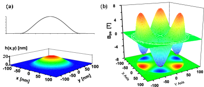
Figure 1: The vertical displacement of our considered systems in the text (a) and the pseudo magnetic fields (b). The radius is $R$=100nm and the height is $h_{0}$=20nm.

Let us consider graphene where mechanical deformation is allowed in a restricted disk shape. This can be realized by a circular hole made in substrate below the graphene sheet, and the deformation is induced through external force. In experiments, circularly symmetric strain fields can be applied by an AFM tip or by a homogeneous gas pressure acting on graphene below the substrateBunch . When strain is induced by homogeneous load, the optimized vertical displacement $h({\bf r})$is given bylandau

$$h({\bf r}) = \frac{f_{0}}{4^{3}D}\left(R^{2}-(x^{2}+y^{2})\right)^{2}\ ,$$ (1)

where $f_{0}$ is the force per unit area acting on surface, $D$ is the bending rigidity, $h_{0}=f_{0}R^{4}/(4^{3}D)$ is the vertical displacement at center, and $R$ is the radius of the region where the deformation is allowed. The in-plane relaxation of the carbon atoms $u_{x},u_{y}$ can be calculated by minimizing the elastic free energy for the given vertical displacement h(r),

$$\textit{F}=\int dxdy\left[\frac{\kappa}{2}(\nabla^{2}h)^{2}+\frac{\lambda}{2}(\sum_{i}u_{ii})^{2}+\mu\sum_{ij}(u_{ij})^{2}\right]$$ (2)

where $\kappa$ is the bending rigidity, $\lambda$ and $\mu(\approx 3\lambda)$ are Lam$\acute{e}$ coefficients, and $u_{ij}$ is the strain tensor. Here, the strain tensor $u_{ij}({\bf r})$ is related to the displacement fields via $u_{xx}=\partial u_{x}/\partial x+\frac{1}{2}(\partial h/\partial x)^{2}$, $u_{yy}=\partial u_{y}/\partial y+\frac{1}{2}(\partial h/\partial y)^{2}$, and $u_{xy}=\frac{1}{2}(\partial u_{x}/\partial y+\partial u_{y}/\partial x)+\frac{1}{2}(\partial h/\partial x)(\partial h/\partial y)$.

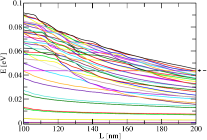
Figure 2: The eigenenergies as a function of the system size $L$. We set $R$=100nm and $h_{0}$=20nm. Note that at certain energy (marked by an arrow), the eigenenergy becomes insensitive to the system size $L$ .

We consider spinless fermions in a graphene lattice. The spinless quasi-particle in the graphene can be described by 4-component wavefunction ${\bf\Psi^{\rm T}}=(\Psi_{K}^{T},\Psi_{-K}^{T})=(\psi_{A,K},\psi_{B,K},\psi_{A,-K},\psi_{B,-K})$. These are the electron wavefunctions near two inequivalent points $\pm K$ in hexagonal Brillouin zone in the two crystalline sublattices A and B. We ignore the valley mixing by the strain based on the results of a tight-binding calculation showing that the two inequivalent valleys are not coupled under uniaxial deformations up to 20% pereira . The main effect of the strain field on the electrons is to modify the energy for electron hopping between the nearest neighbor atoms. The modified quasi-particle energy by the strain is well described by introducing the pseudo gauge field ${\bf A}_{\rm ps}({\bf r})$ in the massless Dirac equation,

$$H=v_{F}\begin{pmatrix}{\vec{\sigma}}\cdot({\bf p}+e{\bf A}_{\rm ps})&0\\ 0&-{\vec{\sigma}}^{*}\cdot({\bf p}-e{\bf A}_{\rm ps})\end{pmatrix}$$ (3)

where $-e$ is the electric charge, $v_{F}\approx 9\times 10^{5}$m/s is the Fermi velocity, ${\bf p}=-i\hbar(\partial_{x},\partial_{y})$, and $\vec{\sigma}=(\sigma_{x},\sigma_{y})$ are Pauli matrices acting in the sublattice space. Here, we take two K points in opposite direction along x-axis. The pseudo gauge field ${\bf A}_{\rm ps}({\bf r})$ is written as

$${\bf A}_{{\rm ps}}=\frac{t\beta}{ev_{F}}(u_{xx}-u_{yy},-2u_{xy}),$$ (4)

where $t\approx 2.8$eV is the electron hopping energy between the nearest $\pi$ orbitals, and $\beta\approx 2-3$ is the dimensionless coupling parameter for the lattice deformationando ; eakim ; manes . In Fig.1, we plot the pseudo magnetic field ${\bf B}_{\rm ps}=B_{\rm ps}{\bf k}=\nabla\times{\bf A}_{\rm ps}$. This is the pseudo magnetic field experienced by the particle in $K$ valley, and for the particle in $-K$ valley, the sign of the magnetic field is opposite.

To investigate the confinement of the quasi-particles in graphene, we compute the eigenenergies of the system as the total graphene size used in the calculation $L$ increases and observe whether the energy is insensitive to the system size. The graphene in the calculation is a disc defined as $r<L$ and the graphene is deformed only in the region of $r<R$. We impose the boundary condition $\Psi_{A}(r=L)=\Psi_{B}(r=L)=0$. While the wavefunctions which extend over the total system are sensitive to the boundary conditions, localized states in the deformed are not affected by the boundary condition. We obtain the eigenvalues of Hamiltonian using basis functions $\psi_{A,B}=\sum c^{A,B}_{n,l}\phi_{n,l}({\bf r})$, where $\phi_{n,l}({\bf r})=J_{l}(\frac{\alpha_{nl}}{L}r)e^{\textit{il}\theta}$. Here, $\alpha_{nl}$ is the n-th zero of the Bessel function $J_{l}(x)$ of order $l$, and we use the indices $l=0,\pm 1,\pm 2,\cdots$, $n=1,2,3,\cdots$.

As shown in Fig.2, we find that at certain energies, there exist eigenstates of which eigenenergies are insensitive to the system size $L$. These are the localized states induced by the deformation of the graphene. Compared to the mid-gap states in a ripple array studied in Ref.guinea08 which shows weak size dependence in logarithmic scale, the eigenenergies of the localized states show almost no size-dependence. From an analytic calculation, the length and energy scales for the localized state can be obtained by bringing the asymptotics of differential equation for the wavefunction to dimensionless form. This is done by rescaling $r\to r_{0}\tilde{r}$, $E\to E_{0}\tilde{E}$, with

$$r_{0}=\left(\frac{\hbar v_{F}R^{4}}{8t\beta h_{0}^{2}}\right)^{1/3},\ \ \ E_{0}=\hbar v_{F}/r_{0}\ .$$ (5)

The scale $r_{0}$ thus plays a role of the localization length and can be estimated as $(R^{4}a/h_{0}^{2})^{1/3}$, where $a$ is the lattice constant. Since the localization length must be shorter than the hole radius, otherwise the Dirac equation with effective magnetic field can not apply, the localization length expressed in the above equation is valid only for strong enough load, $h_{0}\gg\sqrt{Ra}$. The scale $E_{0}$ is associated with the depth of the potential well and the energy of the localized energy levels.

It proves useful to consider the symmetries to understand the energy spectra of quantum systems. The time reversal symmetry is not broken by the strain if we consider the problem with both of the valleys. A time reversal operation defined by

$$\mathcal{T}=\tau_{x}\mathcal{K}$$ (6)

satisfies $\mathcal{T}H\mathcal{T}^{-1}=H,~{}~{}\mathcal{T}i\mathcal{T}^{-1}=-i$bjorken .

Here $\mathcal{K}$ is the complex conjugate operator and $(\tau_{x},\tau_{y},\tau_{z})$ are the Pauli matrices acting in the the valley space. Note that, the Kramers degeneracy is not relevant here since the original system has orthogonal symmetry $\mathcal{T}^{2}=1$.

The quasi-particle can stay in a given valley provided there is no short range scattering ( e.g. lattice defects). In this restricted case, the single valley time reversal symmetry is broken by the pseudo magnetic field. The single valley time reversal operator for 1/2 spin $\mathcal{S}=-i\sigma_{y}\mathcal{K}$ does not commute with the Hamiltonian in Eq.(3). The Hamiltonian is symmetric under the symplectic time reversal transformation only in the absence of the strain ($\mathcal{S}^{2}=-1$); $\mathcal{S}H({\bf A_{\rm ps}}=0)\mathcal{S}^{-1}=-H({\bf A_{\rm ps}}=0)$. The relevant Kramers degeneracy here is lifted by the pseudo magnetic field ${\bf A_{\rm ps}}\neq 0$.

The Hamiltonian in Eq.(3) is also symmetric under a mirror reflection

$$\mathcal{M}=\sigma_{x}\pi_{x},$$ (7)

$$\mathcal{M}H\mathcal{M}^{-1}=H,$$ (8)

where $\pi_{x}$ acts as $x\rightarrow x,~{}~{}y\rightarrow-y$. The valley index remains same under the mirror reflection but inevitably changes lattice index. The spatial symmetry ($|\psi_{A,K}(x,y)|^{2}=|\psi_{B,K}(x,-y)|^{2}$) of the probability density of the localized state shown in Fig. 3 (a) and (b) reflects the $\mathcal{M}$-symmetry in the Hamiltonian.

To understand the electronic structure of the strained graphene, we rewrite the Hamiltonian in Eq.(3) for a given valley $K$ and eigenenegy $E$,

$$\left[v_{F}^{2}\left({\bf p}+e{\bf A_{\rm ps}}\right)^{2}+\hbar ev_{F}^{2}(\nabla\times{\bf A_{\rm ps}})_{z}\sigma_{z}\right]\Psi_{K}=E^{2}\Psi_{K}.$$ (9)

The first term in the left side of Eq.(9) comes from the kinetic energy and the second term is due to the pseudo Zeeman coupling. The pseudo magnetic field is strongest at six points forming a hexagon (Fig. 1) where local Landau levels might be formed. For a given pseudo spin and valley, one can see maximum probability density around only three points (Fig. 3(a) and (b)). This is because of a necessary condition for the stable confinement on the pseudo Zeeman coupling;

$$(\nabla\times{\bf A_{\rm ps}})_{z}\sigma_{z}<0.$$ (10)

In this case, it costs higher energy when a quasi particle to go out to weaker field region. The triangular (instead of hexagonal) shape of the wavefunction for a given lattice and valley is due to the selective stabilization by the pseudo Zeeman coupling.

Figure 3: (a) Probability densities of the localized wavefunctions $|\psi_{A,K}({\bf r})|^{2}$ and (b)$|\psi_{B,K}({\bf r})|^{2}$. We set $R$=100nm, $h_{0}$=20nm. (c) Classical closed orbits of a charged particle in the inhomogeneous magnetic field given by $B_{\rm ps}$ which resemble the probability density of the localized states shown in (a) and (b). (d) Classical paths describing three outgoing channels.

The confinement of channeling in the strained graphene can be visualized by investigating classical trajectories of the charged particles in the pseudo magnetic field (Fig. 3 (c) and (d)). Among the periodic orbits around the pseudo magnetic field maxima, we find clover-shaped orbits which resemble the localized wavefunctions in (Fig. 3 (c)). These closed orbits are very unstable against small perturbation. In quantum mechanics, the clover-shape motion might be responsible for quantum transition between the sites of the local density maxima. We also find out-going trajectories (Fig. 3 (d)) for different initial velocities. A charged particle can propagate along the line where magnetic field changes sign, which is, so called, snake orbitsim . Due to the symmetry of the pseudo magnetic field, there are incoming trajectories in 60 degree rotated angle from those of outgoing trajectories. Quantum mechanically, for given components of lattice and valley, the graphene quantum dot is connected to three incoming and three outgoing chiral channels.

The opening of the channels manifest in the energy spectra. The localized energy level undergoes crossing and avoided crossing as the graphene size $L$ changes. ( see Fig. 2 and Fig. 4 (a) for mode detail.) When the channels open, the eigenenergy of the confined state is affected by the graphene size, so has avoided crossing. Meanwhile when the two level cross each other, the channels remain closed and the eigenenergy of the localized state is insensitive graphene size. In the process of avoided crossing, the confined state undergoes transition to an outer state and a new outer state becomes localized. Since any parity does not change in this continuous process, the confined state transit only to the state with same parity.

Let us consider the response of the strained graphene to real magnetic field. When real magnetic field, ${\bf B}_{\rm re}=\nabla\times{\bf A}_{\rm re}$, is applied, the minimal coupling of the electromagnetic gauge field ${\bf A}_{\rm re}$ is done by replacing ${\bf p}$ with ${\bf p}+e{\bf A}_{\rm real}$ in Eq.(3). The Hamiltonian becomes $H+H^{\prime}$ where

$$H^{\prime}=v_{F}e\begin{pmatrix}{\vec{\sigma}}&0\\ 0&-{\vec{\sigma}}^{*}\end{pmatrix}\cdot{\bf A_{\rm re}},$$ (11)

and ${\bf A_{\rm re}}=\frac{1}{2}(-y,x)B$ is the gauge field for the real magnetic field in z-direction. We want to address here that the application of real magnetic field breaks the time reversal symmetry of the Hamiltonian, but it does not lift the valley degeneracy. This can be proved by showing $<\Psi_{\pm K}|\frac{\partial H^{\prime}}{\partial B}|\Psi_{\pm K}>=0$. The proof comes from the fact the eigenstates have either even or odd parity of the mirror reflection symmetry in Eq.(8), $\mathcal{M}^{2}=1$:

$$<\Psi_{K}|\frac{\partial H^{\prime}}{\partial B}|\Psi_{K}>=<\Psi_{K}|(-y\sigma_{x}+x\sigma_{y})|\Psi_{K}>$$ (12)

$$= <\Psi_{K}|\mathcal{M}(+y\sigma_{x}-x\sigma_{y})\mathcal{M}|\Psi_{K}>$$

$$= -<\Psi_{K}|(-y\sigma_{x}+x\sigma_{y})|\Psi_{K}>.$$

Since $<\Psi_{K}|\frac{\partial H^{\prime}}{\partial B}|\Psi_{K}>$ is equal to its own minus value, it must be zero. The leading magnetic field dependence of the eigenenergy in the presence of magnetic field is not linear but quadratic, $\propto B^{2}$. It comes from the kinetic energy and its sign is positive. Therefore, the orbital magnetization of the strain-induced quantum dot at zero temperature, is diamagnetic ( $-\partial E/\partial B<0$ ) and proportional to the applied magnetic field strength (See Fig. 4 (b)).

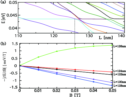
Figure 4: (a) A detailed energy spectra as a function of the system size $L$ which shows crossing and avoided-crossing. (b) The orbital magnetic response, $-\frac{\partial E}{\partial B}$ , of localized states. Mostly the magnetic response is diamagnetic $-\frac{\partial E}{\partial B}<0$ but the response for a level crossing point (indicated by dotted line) shows paramagnetic response (positive value). We set $R$=100nm and $h_{0}$=20nm.

In contrast to the diamagnetic response of the confined state, the orbital magnetic response can be paramagnetic ( $-\partial E/\partial B>0$ ) when there are level-crossings. Near the region of the level crossings, there are two energy levels with opposite parity of $\mathcal{M}$. One of the states is a localized state and the other is a partially opened state (not shown). The accidental degeneracy which happened here can be lifted by applying real magnetic field because $H^{\prime}$ is odd under the mirror reflection, $\mathcal{M}H^{\prime}\mathcal{M}=-H^{\prime}$. Then energy splitting arises, proportional to the real magnetic field strength, which contributes to paramagnetic response.

In conclusion, we have shown that the rotationally symmetric strain in graphene can be considered a quantum dot with spatially separated six chiral channels. The chiral channels exist along the line where the pseudo magnetic field changes sign. The real and pseudo magnetic field has different symmetry under a mirror reflection, which makes the orbital magnetism be diamagnetic or paramagnetic depending on the degeneracy. The orbital magnetic response of the confined state is diamagnetic due to its kinetic energy. When there is an degeneracy with opposite mirror reflection parity, the orbital magnetism can be paramagnetic.

Quite recently, we became aware of a work on dynamics of electrons in strain-induced pseudo magnetic fieldsBlaauboer .

The authors thank M. Sieber, K. Richter, Y. Son, F. Guinea and M. Fogler for useful discussions. This work was supported by the National Research Foundation funded by the Korea government (No.KRF-2008-C00140).

References

- (1) K.S. Novoselov et. al., Science 306, 666 (2004);Nature(London) 438, 197 (2005).
- (2) Y. Zhang, et. al., Nature(London) 438, 201 (2005).
- (3) V. V. Cheianov and V. I. Falko, Phys. Rev. B 74, 041403 (2006); M. I. Katsnelson, K. S. Novoselov and A. K. Geim, Nature physics 2, 620 (2006)
- (4) A. De Martino, L. Dell’Anna, and R. Egger, Phs. Rev. Lett. 98, 066802 (2007).
- (5) G.Giavaras, P. A. Maksym and M. Roy, J. Phys. Condes. Matter 21 102201 (2009)
- (6) D. Wang, G. Jin, Phys. Lett. A, 373, 4082, (2009).
- (7) Vitor M. Pereira, A.H. Castro Neto, Phys. Rev. Lett. 103, 046801 (2009).
- (8) N. Levy et.al., science, 329, 5991 (2010).
- (9) F. Guinea, M. I. Katsnelson, M. A. H. Vozmediano, Phys. Rev. B 77, 075422 (2008).
- (10) Eun-Ah Kim and A. H. Castro Neto, Europhys. Lett., 84, 57007, (2008)
- (11) J.L.Manẽs, Phys. Rev. B, 76, 045430 (2007).
- (12) F. Guinea, B. Horovitz, P. Le Doussal, Phys. Rev. B 77, 205421 (2008).
- (13) A. F. Morpurgo and F. Guinea, Phys. Rev. Lett., 97, 196804 (2006).
- (14) F. Guinea, M.I. Katsnelson, and A. K. Geim, Nature Phys., 6, 30 (2010).
- (15) J. S. Bunch et al., Nano Letters 8, 2458, (2008).
- (16) L.D. Landau and E.M. Lifshitz, Theory of Elasticity, (Pergamon Press Ltd, London, 1959).
- (17) V. M. Pereira and A. H. Castro Neto, Phys. Rev. B 80, 045401 (2009).
- (18) H. Suzuura and T. Ando, Phys. Rev. B 65, 235412 (2002); T. Ando, J. Phys. Soc. Jpn, 75, 124701 (2006).
- (19) J. D. Bjorken and S. D. Drell, Relativistic Quantum Mechanics, McGraw-Hill, (1964), p. 72.
- (20) H.-S. Sim, K.-H. Ahn, K. J. Chang, G. Ihm, N. Kim, and S. J. Lee, Phys. Rev. Lett. 80, 1501 (1998); F. Evers et. al., Phys. Rev. B, 60, 8951 (1999).
- (21) G. M. M. Wakker, R. P. Tiwari, and M. Blaauboer, arXiv:1105.3588.