Maximum lilkelihood estimation in the $\beta$-model

Abstract

We study maximum likelihood estimation for the statistical model for undirected random graphs, known as the $\beta$-model, in which the degree sequences are minimal sufficient statistics. We derive necessary and sufficient conditions, based on the polytope of degree sequences, for the existence of the maximum likelihood estimator (MLE) of the model parameters. We characterize in a combinatorial fashion sample points leading to a nonexistent MLE, and nonestimability of the probability parameters under a nonexistent MLE. We formulate conditions that guarantee that the MLE exists with probability tending to one as the number of nodes increases.

T1Supported in part by Grant FA9550-12-1-0392 from the U.S. Air Force Office of Scientific Research (AFOSR) and the Defense Advanced Research Projects Agency (DARPA), NSF Grant DMS-06-31589, and by a grant from the Singapore National Research Foundation (NRF) under the Interactive & Digital Media Programme Office to the Living Analytics Research Centre (LARC).

, and

1 Introduction

Many statistical models for the representation and analysis of network data rely on information contained in the degree sequence, the vector of node degrees of the observed graph. Node degrees not only quantify the overall connectivity of the network, but also reveal other potentially more refined features of interest. The study of the degree sequences and, in particular, of the degree distributions of real networks is a classic topic in network analysis, which has received extensive treatment in the statistical literature [see, e.g., Holland and Leinhardt (1981), Fienberg and Wasserman (1981a), Fienberg, Meyer and Wasserman (1985)], the physics literature [see, e.g., Newman, Strogatz and Watts (2001), Albert and Barabási (2002), Newman (2003), Park and Newman (2004), Newman, Barabási and Watts (2006), Foster et al. (2007), Willinger, Alderson and Doyle (2009)] as well as in the social network literature [see, e.g., Robins et al. (2007), Goodreau (2007), Handcock and Morris (2007) and references therein]. See also the monograph by Goldenberg et al. (2010) and the books by Kolaczyk (2009), Cohen and Havlin (2010) and Newman (2010).

The simplest instance of a statistical network model based exclusively on the node degrees is the exponential family of probability distributions for undirected random graphs with the degree sequence as its natural sufficient statistic. This is in fact a simpler, undirected version of the broader class of statistical models for directed networks known as the $p_{1}$-models, introduced by Holland and Leinhardt (1981). We will refer to this model as the beta model (henceforth the $\beta$-model), a name recently coined by Chatterjee, Diaconis and Sly (2011), and refer to Blitzstein and Diaconis (2010) for details and extensive references.

Despite its apparent simplicity and popularity, the $\beta$-model, much like most network models, exhibits nonstandard statistical features, since its complexity, measured by the dimension of the parameter space, increases with the size of the graph. Lauritzen (2003, 2008) characterized $\beta$-models as the natural models for representing exchangeable binary arrays that are weakly summarized, that is, random arrays whose distribution only depends on the row and column totals. More recently, Chatterjee, Diaconis and Sly (2011) conducted an analysis of the asymptotic properties of the $\beta$-model, including existence and consistency of the maximum likelihood estimator (MLE) as the dimension of the network increases, and provided a simple algorithm for estimating the natural parameters. They also characterized the graph limits, or graphons [see Lovász and Szegedy (2006)], corresponding to a sequence of $\beta$-models with given degree sequences [for a connection between the theory of graphons and exchangeable arrays see Diaconis and Janson (2008)]. Concurrently, Barvinok and Hartigan (2010) explored the asymptotic behavior of sequences of random graphs with given degree sequences, and studied a different mode of stochastic convergence. Among other things, they show that, as the size of the network increases and under a “tameness” condition, the number of edges of a uniform graph with given degree sequence converges in probability to the number of edges of a random graph drawn from a $\beta$-model parametrized by the MLE corresponding to degree sequence. Yan and Xu (2012) and Yan, Xu and Yang (2012) derived asymptotic conditions for uniform consistency and asymptotic normality of the MLE of the $\beta$-model, and asymptotic normality of the likelihood ratio test for homogeneity of the model parameters. Perry and Wolfe (2012) consider a general class of models for network data parametrized by node-specific parameters, of which the $\beta$-model is a special case. The authors derive nonasymptotic conditions under which the MLEs of model parameters exist and can be well approximated by simple estimators.

In an attempt to avoid the reliance on asymptotic methods, whose applicability to network models remains largely unclear [see, e.g., Haberman (1981)], several researchers have turned to exact inference for the $\beta$-model, which hinges upon the nontrivial task of sampling from the set of graphs with a given degree sequence. Blitzstein and Diaconis (2010) developed and analyzed a sequential importance sampling algorithm for generating a random graph with the prescribed degree sequence [see also Viger and Latapy (2005) for a different algorithm]. Hara and Takemura (2010) and Ogawa, Hara and Takemura (2013) tackled the same task using more abstract algebraic methods, and Petrović, Rinaldo and Fienberg (2010) studied Markov bases for the more general $p_{1}$ model.

In this article we study the existence of the MLE for the parameters of the $\beta$-model under a more general sampling scheme in which each edge is observed a fixed number of times (instead of just once, as in previous works) and for increasing network sizes. We view the issue of existence of the MLE as a natural measure of the intrinsic statistical difficulty of the $\beta$-model for two reasons. First, existence of the MLE is a natural minimum requirement for feasibility of statistical inference in discrete exponential families, such as the $\beta$-model: nonexistence of the MLE is in fact equivalent to nonestimability of the model parameters, as illustrated in Fienberg and Rinaldo (2012). Thus, establishing conditions for existence of the MLE amounts to specifying the conditions under which statistical inference for these models is fully possible. Second, under the asymptotic scenario of growing network sizes, existence of the MLE will provide a natural measure of sample complexity of the $\beta$-model and will indicate the asymptotic scaling of the model parameters for which statistical inference is viable.

Though Chatterjee, Diaconis and Sly (2011) and Barvinok and Hartigan (2010) also considered the existence of the MLE, our analysis differs substantially from theirs in that it is rooted in the statistical theory of discrete linear exponential families and relies in a fundamental way on the geometric properties of these families [see, in particular, Rinaldo, Fienberg and Zhou (2009), Geyer (2009)]. Our contributions are as follows:

• We provide explicit necessary and sufficient conditions for existence of the MLE for the $\beta$-model that are based on the polytope of degree sequences, a well-studied polytope arising in the study of threshold graphs; see Mahadev and Peled (1995). In contrast, the conditions of Chatterjee, Diaconis and Sly (2011) are only sufficient. We then show that nonexistence of the MLE is brought on by certain forbidden patterns of extremal network configurations, which we characterize in a combinatorial way. Furthermore, when the MLE does not exist, we can identify exactly which probability parameters are estimable.

• We use the properties of the polytope of degree sequences to formulate geometric conditions that allow us to derive finite sample bounds on the probability that the MLE does not exist. Our asymptotic results improve analogous results of Chatterjee, Diaconis and Sly (2011) and our proof is both simpler and more direct. Furthermore, we show that the tameness condition of Barvinok and Hartigan (2010) is stronger than our conditions for existence of the MLE.

• Our analysis is not specific to the $\beta$-model but, in fact, follows a principled way for detecting nonexistence of the MLE and identifying nonestimable parameters that is based on polyhedral geometry and applies more generally to discrete models. We illustrate this point by analyzing other network models that are variations or generalizations of the $\beta$-model: the $\beta$-model with random numbers of edges, the Rasch model, the Bradley–Terry model and the $p_{1}$ model. Due to space limitations, the details of these additional analyses are contained in the supplementary material [Rinaldo, Petrović and Fienberg (2013)].

While this is a self-contained article, the results derived here are best understood as applications of the geometric and combinatorial properties of log-linear models under product-multinomial sampling schemes, as detailed in Fienberg and Rinaldo (2012) and its supplementary material, to which we refer the reader for further details as well as for practical algorithms.

The article is organized in the following way. Section 2 introduces the $\beta$-model and establishes the exponential family parametrization that is key to our analysis. In Section 3 we derive necessary and sufficient conditions for existence of the MLE of the $\beta$-model parameters and characterize parameter estimability under a nonexistent MLE. These results are further discussed with examples in Section 4. In Section 5 we provide sufficient conditions on the expected degree sequence guaranteeing that, with high probability as the network size increases, the MLE exists. Finally, in Section 6 we indicate possible extensions of our work and briefly discuss some of the computational issues directly related to detecting nonexistence of the MLE and parameter estimability.

We will assume throughout some familiarity with basic concepts from polyhedral geometry [see, e.g., Schrijver (1986)] and the theory of exponential families; see, for example, Barndorff-Nielsen (1978), Brown (1986).

2 The (generalized) $\beta$-model

In this section we describe the exponential family parametrization of a simple generalization of the $\beta$-model, which, with slight abuse of notation, we will refer to as the $\beta$-model as well.

We are concerned with modeling the occurrence of edges in a simple undirected random graph with node set $\{1,\ldots,n\}$. The statistical experiment consists of recording, for each pair of nodes $(i,j)$ with $i<j$, the number of edges appearing in $N_{i,j}$ i.i.d. samples, where the integers $\{N_{i,j},i<j\}$ are deterministic and positive (we can relax both the nonrandomness and positivity assumptions). Thus, in our setting we allow for the possibility that each edge in the network be sampled a different number of times, a realistic feature that makes the model more flexible. For $i<j$, we denote by $x_{i,j}$, the number of times we observe the edge $(i,j)$ and, accordingly, by $x_{j,i}$ the number of times edge $(i,j)$ is missing. Thus, for all $(i,j)$,

$$x_{i,j}+x_{j,i}=N_{i,j}.$$

We model the observed edge counts $\{x_{i,j},i<j\}$ as draws from mutually independent binomial distributions, with $x_{i,j}\sim\operatorname{Bin}(N_{i,j},p_{i,j})$, where $p_{i,j}\in(0,1)$ for each $i<j$.

Data arising from such an experiment has a representation in the form of a $n\times n$ contingency table with empty diagonal cells and whose $(i,j)$th cell contains the count $x_{i,j}$, $i\neq j$. For modeling purposes, however, we need only consider the upper-triangular part of this table. Indeed, since, given $x_{i,j}$, the value of $x_{j,i}$ is determined by $N_{i,j}-x_{i,j}$, we can represent the sample space more parsimoniously as the following subset of $\mathbb{N}^{n\choose 2}$:

$$\mathcal{S}_{n}:=\bigl{\{}x_{i,j}\dvtx i<j\mbox{ and }x_{i,j}\in\{0,1,\ldots,N_{i,j}\}\bigr{\}}.$$

We index the coordinates $\{(i,j)\dvtx i<j\}$ of any point in $\mathcal{S}_{n}$ lexicographically.

In the $\beta$-model, we parametrize the ${n\choose 2}$ edge probabilities by points $\beta\in\mathbb{R}^{n}$ as follows. For each $\beta\in\mathbb{R}^{n}$, the probability parameters are uniquely determined as

$$p_{i,j}=\frac{e^{\beta_{i}+\beta_{j}}}{1+e^{\beta_{i}+\beta_{j}}}\quad\mbox{and}\quad p_{j,i}=1-p_{i,j}=\frac{1}{1+e^{\beta_{i}+\beta_{j}}}\qquad\forall i\neq j$$ (1)

or, equivalently, in terms of log-odds,

$$\log\frac{p_{i,j}}{1-p_{i,j}}=\beta_{i}+\beta_{j}\qquad\forall i\neq j.$$ (2)

The magnitude and sign of $\beta_{i}$ quantifies the propensity of node $i$ to have ties: the degree of node $i$ is expected to be large (small) if $\beta_{i}$ is positive (negative) and of large magnitude. Thus the $\beta$-model is the natural heterogenous version of the well-known Erdős–Rényi random graph model [Erdős and Rényi (1959)]. For a discussion of this model and its generalizations see Goldenberg et al. (2010).

For a given choice of $\beta$, the probability of observing the vector of edge counts $x\in\mathcal{S}_{n}$ is

$$p_{\beta}(x)=\prod_{i<j}\pmatrix{N_{i,j}\cr x_{i,j}}p_{i,j}^{x_{i,j}}(1-p_{i,j})^{N_{i,j}-x_{i,j}}$$ (3)

with the probability values $p_{i,j}$ satisfying (1). Simple algebra allows us to rewrite this expression in exponential family form as

$$p_{\beta}(x)=\exp\Biggl{\{}\sum_{i=1}^{n}d_{i}\beta_{i}-\psi(\beta)\Biggr{\}}\prod_{i<j}\pmatrix{N_{i,j}\cr x_{i,j}},$$ (4)

where the coordinates of the vector of the minimal sufficient statistics $d=d(x)\in\mathbb{N}^{n}$ are

$$d_{i}=\sum_{j<i}x_{j,i}+\sum_{j>i}x_{i,j},\qquad i=1,\ldots,n,$$ (5)

and the log-partition function is $\psi(\beta)=\sum_{i<j}N_{i,j}\log(1+e^{\beta_{i}+\beta_{j}})$.

Note that $e^{\psi(\beta)}<\infty$ for all $\beta\in\mathbb{R}^{n}$, so $\mathbb{R}^{n}$ is the natural parameter space of the full and steep exponential family with support $\mathcal{S}_{n}$ [see, e.g., Barndorff-Nielsen (1978)] and densities given by the exponential term in (4).

Random graphs with fixed degree sequence

When $N_{i,j}=1$ for all $(i,j)$, the support $\mathcal{S}_{n}$ reduces to the set $\mathcal{G}_{n}:=\{0,1\}^{n\choose 2}$, which encodes all undirected simple graphs on $n$ nodes: for any $x\in\mathcal{G}_{n}$, the corresponding graph has an edge between nodes $i$ and $j$, with $i<j$, if and only if $x_{i,j}=1$. In this case, the $\beta$-model yields a class of distributions for random undirected simple graphs on $n$ nodes, where the edges are mutually independent Bernoulli random variables with probabilities of success $\{p_{i,j},i<j\}$ satisfying (1). Then, by (5), the $i$th minimal sufficient statistic $d_{i}$ is the degree of node $i$, that is, the number of nodes adjacent to $i$, and the vector $d(x)$ of sufficient statistics is the degree sequence of the observed graph $x$. This is the version of the $\beta$-model studied by Chatterjee, Diaconis and Sly (2011).

3 Existence of the MLE for the $\beta$-model

We now derive a necessary and sufficient condition for the existence of the MLE of the natural parameter $\beta$ or, equivalently, of the probability parameters $\{p_{i,j},i<j\}$ as defined in (1). For a given $x\in\mathcal{S}_{n}$, we say that the MLE does not exist when

$$\Bigl{\{}\beta^{*}\dvtx p_{\beta^{*}}(x)=\sup_{\beta\in\mathbb{R}^{n}}p_{\beta}(x)\Bigr{\}}=\varnothing,$$

where $p_{\beta}(x)$ is given in (4). For the natural parameters, nonexistence of the MLE implies that we cannot attain the supremum of the likelihood function (4) by any finite vector in $\mathbb{R}^{n}$. For the probability parameters, nonexistence signifies that the supremum of (3) cannot be attained by any set of probability values bounded away from $0$ and $1$, and satisfying the equations from (1). Either way, nonexistence of the MLE implies that only a random subset of the model parameters is estimable; see Fienberg and Rinaldo (2012).

Our analysis on the existence of the MLE and parameter estimability for the $\beta$-model is based on a geometric object that plays a key role throughout the rest of the paper: the polytope of degree sequences. To this end, we note that, for each $x\in\mathcal{S}_{n}$, we can obtain the vector of sufficient statistics $d(x)$ for the $\beta$-model as

$$d(x)=\mathrm{A}x,$$

where $\mathrm{A}$ is the $n\times{n\choose 2}$ design matrix equal to the node-edge incidence matrix of a complete graph on $n$ nodes. Specifically, we index the rows of $\mathrm{A}$ by the node labels $i\in\{1,\ldots,n\}$, and the columns by the set of all pairs $(i,j)$ with $i<j$, ordered lexicographically. The entries of $\mathrm{A}$ are ones along the coordinates $(i,(i,j))$ and $(j,(i,j))$ for $i<j$, and zeros otherwise. For instance, when $n=4$

$$\mathrm{A}=\left[\matrix{1&1&1&0&0&0\cr 1&0&0&1&1&0\cr 0&1&0&1&0&1\cr 0&0&1&0&1&1}\right],$$

where we index the columns lexicographically by the pairs $(1,2)$, $(1,3)$, $(1,4)$, $(2,3)$, $(2,4)$ and $(3,4)$. In particular, for any undirected simple graph $x\in\mathcal{G}_{n}$, $\mathrm{A}x$ is the associated degree sequence. The polytope of degree sequences $P_{n}$ is the convex hull of all possible degree sequences, that is,

$$P_{n}:=\operatorname{convhull}\bigl{(}\{\mathrm{A}x,x\in\mathcal{G}_{n}\}\bigr{)}.$$

The integral polytope $P_{n}$ is a well-studied object in graph theory; for example, see Chapter 3 in Mahadev and Peled (1995). In particular, when $n=2$, $P_{n}$ is just a line segment in $\mathbb{R}^{2}$ connecting the points $(0,0)$ and $(1,1)$, while, for all $n\geq 3$, $\operatorname{dim}(P_{n})=n$.

We now fully characterize the existence of the MLE for the $\beta$-model using the polytope of degree sequences in the following fashion. For any $x\in\mathcal{S}_{n}$, let

$$\tilde{p}_{i,j}:=\frac{x_{i,j}}{N_{i,j}},\qquad i<j,$$

and set $\tilde{d}=\tilde{d}(x)\in\mathbb{R}^{n}$ to be the vector with coordinates

$$\tilde{d}_{i}:=\sum_{j<i}\tilde{p}_{j,i}+\sum_{j>i}\tilde{p}_{i,j},\qquad i=1,\ldots,n,$$ (6)

a rescaled version of the sufficient statistics (5), normalized by the number of observations. In particular, for the random graph model, $\tilde{d}=d$.

Theorem 3.1

Let $x\in\mathcal{S}_{n}$ be the observed vector of edge counts. The MLE exists if and only if $\tilde{d}(x)\in\operatorname{int}(P_{n})$.

Theorem 3.1 verifies the conjecture contained in Addendum A in Chatterjee, Diaconis and Sly (2011) for the random graph model: the MLE exists if and only if the degree sequence belongs to the interior of $P_{n}$. This result follows from the standard properties of exponential families; see Theorem 9.13 in Barndorff-Nielsen (1978) or Theorem 5.5 in Brown (1986). It also confirms the observation made by Chatterjee, Diaconis and Sly (2011) that the MLE never exists if $n=3$: indeed, since $P_{3}$ has exactly $8$ vertices, as many as the possible graphs on $3$ nodes, no degree sequence can be inside $P_{3}$.

We conclude by taking note that, by representing the sufficient statistics as a linear mapping $d=\mathrm{A}x$, we can recast the $\beta$-model as a log-linear model with design matrix $\mathrm{A}^{\top}$ and product-multinomial scheme, with ${n\choose 2}$ sampling constraints, one for each edge. This simple yet far reaching observation allows us, among the other things, to design algorithms for detecting nonexistence of the MLE and identifying estimable parameters under a nonexistent MLE, as explained in the supplementary material to this article.

3.1 Parameter estimability under a nonexistent MLE

The geometric nature of Theorem 3.1 has important consequences. First, it allows us to identify the patterns of observed edge counts that cause nonexistence of the MLE; that is, the sample points for which the MLE is undefined. Second, it yields a complete description of estimability of the edge probability parameters under a nonexistent MLE, a key issue for correct evaluation of degrees of freedom of the model. The next result addresses the last two points.

Lemma 3.2

A point $y$ belongs to the interior of some face $F$ of $P_{n}$ if and only if there exists a set $\mathcal{F}\subset\{(i,j),i<j\}$ such that

$$y=\mathrm{A}p,$$ (7)

where $p=\{p_{i,j}\dvtx i<j,p_{i,j}\in[0,1]\}\in\mathbb{R}^{{n\choose 2}}$ is such that $p_{i,j}\in\{0,1\}$ if $(i,j)\notin\mathcal{F}$ and $p_{i,j}\in(0,1)$ if $(i,j)\in\mathcal{F}$. The set $\mathcal{F}$ is uniquely determined by the face $F$ and is the maximal set for which (7) holds.

Following Geiger, Meek and Sturmfels (2006) and Fienberg and Rinaldo (2012), we refer to any such set $\mathcal{F}$ a facial set of $P_{n}$ and its complement, $\mathcal{F}^{c}=\{(i,j)\dvtx i<j\}\setminus\mathcal{F}$, a co-facial set. Facial sets form a lattice that is isomorphic to the face lattice of $P_{n}$ [Fienberg and Rinaldo (2012), Lemma 5]. Thus the faces of $P_{n}$ are in one-to-one correspondence with the facial sets of $P_{n}$ and, for any pair of faces $F$ and $F^{\prime}$ of $P_{n}$ with associated facial sets $\mathcal{F}$ and $\mathcal{F}^{\prime}$, $F\cap F^{\prime}=\varnothing$ if and only if $\mathcal{F}\cap\mathcal{F}^{\prime}=\varnothing$ and $F\subset F^{\prime}$ if and only if $\mathcal{F}\subset\mathcal{F}^{\prime}$. In details, for a point $x\in\mathcal{S}_{n}$, $d(x)=\mathrm{A}x$ belongs to the interior of a face $F$ of $P_{n}$ if and only if there exists a nonnegative $p$ such that $d(x)=\mathrm{A}p$, where $\mathcal{F}=\{(i,j)\dvtx 0<p_{i,j}<1\}$ is the facial set corresponding to $F$. By the same token, $y\in\operatorname{int}(P_{n})$ if and only if $y=\mathrm{A}p$ for a vector $p$ with coordinates strictly between $0$ and $1$.

Facial sets have statistical relevance for two reasons. First, nonexistence of the MLE can be described combinatorially in terms of co-facial sets, that is, patterns of edge counts that are either $0$ or $N_{i,j}$. In particular, the MLE does not exist if and only if the set $\{(i,j)\dvtx i<j,x_{i,j}=0$ or $N_{i,j}\}$ contains a co-facial set. Second, apart from exhausting all possible patterns of forbidden entries in the table leading to a nonexistent MLE, facial sets specify which probability parameters are estimable. In fact, inspection of the likelihood function (3) reveals that, for any observable set of counts $\{x_{i,j}\dvtx i<j\}$, there always exists a unique maximizer $\widehat{p}=\{\widehat{p}_{i,j},i<j\}$ which, by strict concavity, is uniquely determined by the first order optimality conditions

$$\tilde{d}(x)=\mathrm{A}\widehat{p},$$

also known as the moment equations. Existence of the MLE is then equivalent to $0<\widehat{p}_{i,j}<1$ for all $i<j$. When the MLE does not exist, that is, when $\tilde{d}$ is on the boundary of $P_{n}$, the moment equations still hold, but the entries of the optimizer $\{\widehat{p}_{i,j},i<j\}$, known as the extended MLE, are no longer strictly between $0$ and $1$. Instead, by Lemma 3.2, the extended MLE is such that $\widehat{p}_{i,j}=\tilde{p}_{i,j}\in\{0,1\}$ for all $(i,j)\in\mathcal{F}^{c}$. Furthermore, it is possible to show [see, e.g., Morton (2013)] that $\widehat{p}_{i,j}\in(0,1)$ for all $(i,j)\in\mathcal{F}$. Therefore, when the MLE does not exist, only the probabilities $\{p_{i,j},(i,j)\in\mathcal{F}\}$ are estimable by the extended MLE. We refer the reader to Barndorff-Nielsen (1978), Brown (1986), Fienberg and Rinaldo (2012) and references therein, for details about the theory of extended exponential families and extended maximum likelihood estimation in log-linear models.

To summarize, while co-facial sets encode the patterns of table entries leading to a nonexistent MLE, facial sets indicate which probability parameters are estimable. A similar, though more involved interpretation holds for the estimability of the natural parameters, for which the reader is referred to Fienberg and Rinaldo (2012). Further, for a given sample point $x$, the realized facial set and its cardinality are both random, as they depend on the actual value of the observed sufficient statistics $\mathrm{A}x$. This implies that, with a nonexistent MLE, the set of estimable parameters is itself random.

4 The boundary of $P_{n}$

Theorem 3.1 and Lemma 3.2 show that the boundary of the polytope $P_{n}$ plays a fundamental role in determining the existence of the MLE for the $\beta$-model and in specifying which parameters are estimable. In particular, the larger the number of faces (i.e., facial sets) of $P_{n}$ the higher the complexity of the $\beta$-model as measured by the numbers of possible patterns of edge counts for which the MLE does not exist. Therefore, gaining an even basic understanding of the number and of the types of co-facial patterns will provide valuable insights into the behavior of the $\beta$-model. Below we further elaborate on the consequences of the results established in Section 3 and present a small selection of examples of co-facial sets associated to the facets of $P_{n}$.

Though the discussion and examples of this section will reveal a number of subtle issues, we believe that the key message is two-fold. First, the combinatorial complexity of $P_{n}$, measured by both the number of the types of co-facial sets, grows very fast with $n$, with the co-facial sets associated to node degrees bounded away from $0$ and $n-1$ vastly outnumbering the easily detectable cases of minimal or maximal degree. Second, since complete enumeration of the faces of $P_{n}$ is impractical, it is important to devise algorithms for detecting a nonexistent MLE and identifying the facial sets of estimable parameters. Both these issues become more severe in large and sparse networks, where it is expected that the exploding number of possible nontrivial co-facial set renders estimation of the model parameters more difficult. Later in Section 5, we will derive conditions, based on the geometry of $P_{n}$ that prevents this from happening, with large probability for large $n$.

4.1 The combinatorial complexity of $P_{n}$

Mahadev and Peled (1995) describe the facet-defining inequalities of $P_{n}$, for all $n\geq 4$ (when $n\leq 3$ the problem is of little interest), a result we use later in Section 5. Let $\mathcal{P}$ be the set of all pairs $(S,T)$ of disjoint nonempty subsets of $\{1,\ldots,n\}$, such that $|S\cup T|\in\{2,\ldots,n-3,n\}$. For any $(S,T)\in\mathcal{P}$ and $y\in P_{n}$, let

$$g(S,T,y,n):=|S|\bigl{(}n-1-|T|\bigr{)}-\sum_{i\in S}y_{i}+\sum_{i\in T}y_{i}.$$ (8)

Theorem 4.1 ([Theorem 3.3.17 in Mahadev and Peled (1995)])

Let $n\geq 4$ and $y\in P_{n}$. The facet-defining inequalities of $P_{n}$ are: [(iii)]

$y_{i}\geq 0$, for $i=1,\ldots,n$;

$y_{i}\leq n-1$, for $i=1,\ldots,n$;

$g(S,T,y,n)\geq 0$, for all $(S,T)\in\mathcal{P}$.

Even with the exhaustive characterization of $P_{n}$ provided by Theorem 4.1, understanding the combinatorial complexity of $P_{n}$ (i.e., the collection of all its faces and their inclusion relations) is far from trivial. Stanley (1991) studied the number faces of the polytope of degree sequences $P_{n}$ and derived an expression for computing the entries of the $f$-vector of $P_{n}$. The $f$-vector of an $n$-dimensional polytope is the vector of length $n$ whose $i$th entry contains the number of $i$-dimensional faces, $i=0,\ldots,n-1$. For example, the $f$-vector of $P_{8}$ is the $8$-dimensional vector

$$(334\mbox{,}982,1\mbox{,}726\mbox{,}648,3\mbox{,}529\mbox{,}344,3\mbox{,}679\mbox{,}872,2\mbox{,}074\mbox{,}660,610\mbox{,}288,81\mbox{,}144,3322).$$

Thus, $P_{8}$ is an $8$-dimensional polytope with $334\mbox{,}982$ vertices, $1\mbox{,}726\mbox{,}648$ edges and so on, up to $3322$ facets. Also, according to Stanley’s formula, the number of facets of $P_{4}$, $P_{5}$, $P_{6}$ and $P_{7}$ are $22$, $60$, $224$ and $882$, respectively [these numbers correspond to the numbers we obtained with the software polymake, using the methods described in the supplementary material to this article; see Gawrilow and Joswig (2000)]. Stanley’s analysis showed that the combinatorial complexity of $P_{n}$ is extraordinarily large, with both the number of vertices, and the number of facets growing at least exponentially in $n$, and consequently, the tasks of identifying points on the boundary of $P_{n}$ and the associated facial set are far from trivial. For instance, computing directly the number of vertices of $P_{10}$ is prohibitively expensive, even using one of the best known algorithms, such as the one implemented in the software minksum; see Weibel (2010). To overcome these problems we have devised an algorithm for detecting boundary points and the associated facial sets that can handle networks with up to hundreds of nodes. We report on this algorithm, which is based on a log-linear model reparametrization and is equivalent to what is known in computational geometry as the “Cayley trick,” in the supplementary material. Using the methods described there, we were able to identify a few interesting cases in which the MLE does not exist, most of which have gone unrecognized in the statistical literature. Below we describe some of our computations for the purpose of elucidating the results derived in Section 3.

4.2 Some examples of co-facial sets

Recall that we can represent the data as a $n\times n$ table of counts with structural zero diagonal elements and where the $(i,j)$th entry of the table indicates the number of times, out of $N_{i,j}$, in which we observed the edges $(i,j)$. In our examples, empty cells correspond to facial sets and may contain arbitrary count values, in contrast to the cells in the co-facial sets that contain either a zero value or a maximal value, namely $N_{i,j}$. Lemma 3.2 implies that extreme count values of this nature are precisely what leads to the nonexistence of the MLE. The pattern shown on the left of Table 1 provides an instance of a co-facial set, which corresponds to a facet of $P_{4}$. Assume for simplicity that the empty cells contain counts bounded away

=280pt $\times$ 0 $N_{1,2}$ $\times$ $\times$ $N_{3,4}$ 0 $\times$ $\times$ 0 1 2 3 $\times$ 2 1 2 1 $\times$ 3 1 2 0 $\times$ $\times$ 0 0.5 0.5 1 $\times$ 0.5 0.5 0.5 0.5 $\times$ 1 0.5 0.5 0 $\times$

Table 1: Left: co-facial set leading to a nonexistent MLE. Center: an example of data exhibiting the pattern of counts consistent with the co-facial set on the left when $N_{i,j}=3$ for all $i\neq j$. Right: table of the extended MLE of the estimated probabilities

from 0 and $N_{i,j}$. Then the sufficient statistics $\tilde{d}$ are also bounded away from $0$ and $n-1$, and so are the row and column sums of the normalized counts $\{\frac{x_{i,j}}{N_{i,j}}\dvtx i\neq j\}$, yet the MLE does not exist. This is further illustrated in Table 1, center, which shows an instance of data with $N_{i,j}=3$ for all $i\neq j$, satisfying the above pattern and, on the right, the probability values

=280pt $\times$ 0 $N_{1,2}$ $\times$ 0 0 $N_{3,2}$ $\times$ $N_{4,2}$ $\times$ $\times$ 0 0 $N_{1,2}$ $\times$ 0 $\times$ $N_{4,1}$ $N_{4,2}$ $\times$

Table 2: Examples of a co-facial set leading to a nonexistent MLE.Left: $\tilde{d}_{2}=0$. Right: example where the degrees are all bounded away from $0$ and $3$, the MLE does not exist

maximizing the log-likelihood function. Notice that, because the MLE does not exist, the supremum of the log-likelihood under the natural parametrization is attained in the limit by any sequence of natural parameters $\{\beta^{(k)}\}$ of the form $\beta^{(k)}=(-c_{k},-c_{k},c_{k},c_{k})$, where $c_{k}\rightarrow\infty$ as $k\rightarrow\infty$. As a result, some of these probability values are $0$ and $1$. The order of the pattern is crucial. In Table 2 we show, on the left, another example of a co-facial set that is easy to detect, since it corresponds to a value of $0$ for the normalized sufficient statistic $\tilde{d}_{2}$. Indeed, from cases (i) and (ii) of Theorem 4.1, the MLE does not exist if $\tilde{d}_{i}=0$ or $\tilde{d}_{i}=n-1$, for some $i$. On the right, we show a co-facial set that is instead compatible with normalized sufficient statistics being bounded away from $0$ and $n-1$. Finally, in Table 3 we list all 22 co-facial sets associated with the facets of $P_{4}$, including the cases already shown.

Table 3: All possible co-facial sets for $P_{4}$ corresponding to the facets of $P_{4}$(empty cells indicate arbitrary entry values)

$\times$ 0 $N_{1,2}$ $\times$ $\times$ $N_{3,4}$ 0 $\times$	$\times$ 0 $N_{1,2}$ $\times$ 0 0 $N_{3,2}$ $\times$ $N_{4,2}$ $\times$	$\times$ 0 0 $N_{1,2}$ $\times$ 0 $\times$ $N_{4,1}$ $N_{4,2}$ $\times$
$\times$ 0 0 0 $N_{1,2}$ $\times$ $N_{1,3}$ $\times$ $N_{4,1}$ $\times$	$\times$ 0 0 $N_{1,2}$ $\times$ 0 $N_{1,3}$ $N_{2,3}$ $\times$ $\times$	$\times$ 0 0 $\times$ $N_{1,3}$ $\times$ 0 $N_{1,4}$ $N_{3,4}$ $\times$
$\times$ 0 $\times$ 0 $N_{1,3}$ $N_{2,3}$ $\times$ 0 $N_{3,4}$ $\times$	$\times$ $N_{1,2}$ $N_{1,3}$ $N_{1,4}$ 0 $\times$ 0 $\times$ 0 $\times$	$\times$ $N_{1,3}$ $N_{1,4}$ $\times$ 0 $\times$ $N_{3,4}$ 0 0 $\times$
$\times$ $N_{1,2}$ $N_{1,3}$ 0 $\times$ $N_{2,3}$ 0 0 $\times$ $\times$	$\times$ $N_{1,3}$ $\times$ $N_{2,3}$ 0 0 $\times$ $N_{3,4}$ 0 $\times$	$\times$ $N_{1,2}$ $N_{1,4}$ 0 $\times$ $N_{2,4}$ $\times$ 0 0 $\times$
$\times$ $N_{1,4}$ $\times$ $N_{2,4}$ $\times$ $N_{3,4}$ 0 0 0 $\times$	$\times$ 0 $\times$ 0 $N_{1,3}$ $N_{2,3}$ $\times$ 0 $N_{3,4}$ $\times$	$\times$ $N_{1,2}$ 0 $\times$ 0 0 $N_{2,3}$ $\times$ $N_{2,4}$ $\times$
$\times$ $\times$ 0 0 $N_{2,3}$ $\times$ 0 $N_{2,4}$ $N_{3,4}$ $\times$	$\times$ 0 $\times$ 0 $\times$ 0 $N_{1,4}$ $N_{2,4}$ $N_{3,4}$ $\times$	$\times$ $N_{1,2}$ 0 $\times$ $\times$ 0 $N_{3,4}$ $\times$
$\times$ 0 $\times$ $N_{2,4}$ $N_{1,3}$ $\times$ 0 $\times$	$\times$ $N_{1,3}$ $\times$ 0 0 $\times$ $N_{2,4}$ $\times$	$\times$ $N_{1,4}$ $\times$ 0 $N_{2,3}$ $\times$ 0 $\times$
	$\times$ 0 $\times$ $N_{2,3}$ 0 $\times$ $N_{1,4}$ $\times$

In general, there are $2n$ facets of $P_{n}$ that are determined by one $\tilde{d}_{i}$ equal to $0$ or $n-1$. Thus, just by inspecting the row sums or the observed sufficient statistics, we can detect only $2n$ co-facial sets associated to as many facets of $P_{n}$. Comparing this number to the entries of the $f$-vector calculated in Stanley (1991), however, and as our computations confirm, most of the facets of $P_{n}$ do not yield co-facial sets of this form. Since the number of facets appears to grow exponentially in $n$, we conclude that most of the co-facial sets do not appear to arise in this fashion. Thus, at least combinatorially, patterns of data counts leading to the nonexistence of MLEs but with the normalized degree bounded away from $0$ and $n-1$ are much more frequent, especially in larger networks.

4.3 The random graph case

In the special case of $N_{i,j}=1$ for all $i<j$, which is equivalent to a model for random undirected graphs, points on the boundary of $P_{n}$ are, by construction, degree sequences and have a direct graph-theoretical interpretation. We say that a subset of a set of nodes of a given graph is stable if it induces a subgraph with no edges and a clique if it induces a complete subgraph.

Lemma 4.2 ([Lemma 3.3.13 in Mahadev and Peled (1995)])

Let $d$ be a degree sequence of a graph $\mathcal{G}$ that lies on the boundary of $P_{n}$. Then either $d_{i}=0$, or $d_{i}=n-1$ for some $i$, or there exist nonempty and disjoint subsets $S$ and $T$ of $\{1,\ldots,n\}$ such that:

1. [(4)]

2. $S$ is clique of $\mathcal{G}$;

3. $T$ is a stable set of $\mathcal{G}$;

4. every vertex in $S$ is adjacent to every vertex in $(S\cup T)^{c}$ in $\mathcal{G}$;

5. no vertex of $T$ is adjacent to any vertex of $(S\cup T)^{c}$ in $\mathcal{G}$.

Using Lemma 4.2, we can create virtually any example of a random graph whose node degree sequence lies on the boundary of $P_{n}$. In particular, we note that having node degrees bounded away from $0$ and $n-1$ is not a sufficient condition for the existence of the MLE, although its violation implies nonexistence of the MLE; see the examples of Figure 1. Nonetheless, Lemma 4.2 is of little or no practical use when it comes to detecting boundary points and the associated co-facial sets, since checking for the existence of a pair $(S,T)$ of subsets of nodes satisfying conditions (1) through (4) is algorithmically impractical. In the supplementary material to this article, we describe alternative procedures that can be used in large networks.

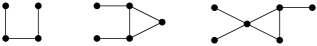
Figure 1: Examples of random graphs on $4$ (left), $5$ (center) and $6$ (right) nodes with node degrees bounded away from $0$ and $n-1$ and for which the MLE is not defined. Lemma 4.2 applies with $S=\{3,4\}$ and $T=\{1,2\}$ (left), with $S=\{2,3,4\}$ and $T=\{1,5\}$ (center) and with $S=\{1,2,6\}$ and $T=\{3,4,5\}$ (right).

Figure 1 shows three examples of graphs on $4$, $5$ and $6$ nodes for which the MLE of the $\beta$-model is undefined even though the node degrees are bounded away from $0$ and $n-1$ in all cases. All the examples were constructed using directly Lemma 4.2, as explained in the caption. To the best of our knowledge, even these very small examples of nonexistent MLEs are unknown to practitioners and no available software for fitting the MLE is able to detect nonexistence, much less identify the relevant facial set.

For the case $n=4$, our computations show that there are $14$ distinct co-facial sets associated to the facets of $P_{n}$. Eight of them correspond to degree sequences containing a $0$ or a $3$, and the remaining six are shown in Table 4, which we computed numerically using the procedure described in the supplementary

Table 4: Patterns of zeros and ones yielding random graphs with nonexistent MLE(empty cells indicate that the entry could be a $0$ or a $1$)

$\times$ 0 1 $\times$ $\times$ 1 0 $\times$	$\times$ 0 $\times$ 1 $\times$ 1 0 $\times$	$\times$ 1 $\times$ 0 1 $\times$ 0 $\times$
$\times$ 1 0 $\times$ $\times$ 0 1 $\times$	$\times$ 1 $\times$ 0 $\times$ 0 1 $\times$	$\times$ 0 $\times$ 1 0 $\times$ 1 $\times$

material. Notice that the three tables on the second row are obtained from the first three tables by switching zeros with ones. Furthermore, the number of the co-facial sets we found is smaller than the number of facets of $P_{n}$, which is $22$, as shown in Table 3. This is a consequence of the fact that the only observed counts in the random graph model are $0$’s or $1$’s: it is in fact easy to see in Table 3 that any co-facial set containing three zero counts and three maximal counts $N_{i,j}$ is equivalent, in the random graph case, to a node having degree zero or $3$. However, as soon as $N_{i,j}\geq 2$, the number of possible co-facial sets matches the number of faces of $P_{n}$. Therefore, the condition $N_{i,j}=1$ is not inconsequential, as it appears to reduce the numbers of observable patterns leading to a nonexistent MLE, though we do not know the extent of the impact of such reduction in general.

5 Existence of the MLE: Finite sample bounds

In this section we exploit the geometry of the boundary of $P_{n}$ from Lemma 4.2 to derive sufficient conditions that imply the existence of the MLE with large probability as the size of the network $n$ grows. These conditions essentially guarantee that the probability of observing any of the super-exponentially many (in $n$) co-facial sets of $P_{n}$ is polynomially small in $n$. Unlike in previous analyses, our result does not require the network to be dense.

We make the simplifying assumption that $N_{i,j}=N$, for all $i$ and $j$, where $N=N(n)\geq 1$ could itself depend on $n$. Recall the random vector $\tilde{d}$, whose coordinates are given in (6) and let $\overline{d}=\mathbb{E}[\tilde{d}]\in\mathbb{R}^{n}$ be its expected value under the $\beta$-model. Then

$$\overline{d}_{i}=\sum_{j<i}p_{j,i}+\sum_{j>i}p_{i,j},\qquad i=1,\ldots,n.$$

We formulate sufficient conditions for the existence of the MLE in terms of the entries of the vector $\overline{d}$.

Theorem 5.1

Assume that, for all $n\geq\max\{4,2\sqrt{c\frac{n\log n}{N}}+1\}$, the vector $\overline{d}$ satisfies the conditions: [(ii)]

$\min_{i}\min\{\overline{d}_{i},n-1-\overline{d}_{i}\}\geq 2\sqrt{c\frac{n\log n}{N}}+C$,

$\min_{(S,T)\in\mathcal{P}}g(S,T,\overline{d},n)>|S\cup T|\sqrt{c\frac{n\log n}{N}}+C$, where $c>1/2$ and $C\in(0,\frac{n-1}{2}-\sqrt{c\frac{n\log n}{N}})$. Then, with probability at least $1-\frac{2}{n^{2c-1}}$, the MLE exists.

When $N$ is constant, for example, when $N=1$ as in the random graph case, we can relax the conditions of Theorem 5.1 by requiring condition (ii) to hold only over subsets $S$ and $T$ of cardinality of order $\Omega(\sqrt{n\log n})$. While we present this result in greater generality by assuming only that $n\geq N$, we do not expect it to be sharp in general when $N$ grows with $n$.

Corollary 5.2

Let $n\geq\max\{N,4,2\sqrt{cn\log n}+1\}$, $c>1$ and $C\in(0,\frac{n-1}{2}-\sqrt{cn\log n})$. Assume the vector $\overline{d}$ satisfies the conditions: [(ii^′)]

$\min_{i}\min\{\overline{d}_{i},n-1-\overline{d}_{i}\}\geq 2\sqrt{cn\log n}+C$,

$\min_{(S,T)\in\mathcal{P}_{n}}g(S,T,\overline{d},n)>|S\cup T|\sqrt{cn\log n}+C$, where

$$\mathcal{P}_{n}:=\bigl{\{}(S,T)\in\mathcal{P}\dvtx\min\bigl{\{}|S|,|T|\bigr{\}}>\sqrt{cn\log n}+C\bigr{\}},$$

where the set $\mathcal{P}$ was defined before Theorem 4.1. Then the MLE exists with probability at least $1-\frac{2}{n^{2c-2}}$. If $N=1$, it is sufficient to have $c>1/2$, and the MLE exists with probability larger than $1-\frac{2}{n^{2c-1}}$.

Discussion and comparison with previous work

Since $|S\cup T|\leq n$, one could replace assumption (ii) of Theorem 5.1 with the simpler but stronger condition

$$\min_{(S,T)\in\mathcal{P}_{n}}g(S,T,\overline{d},n)>n^{3/2}\sqrt{c\log n}+C_{n}.$$

Then, if we assume for simplicity that $N$ is a constant, as in Corollary 5.2, the MLE exists with probability tending to one at a rate that is polynomial in $n$ whenever

$$\min_{i}\min\{\overline{d}_{i},n-1-\overline{d}_{i}\}=\Omega(\sqrt{n\log n})$$

and, for all pairs $(S,T)\in\mathcal{P}$,

$$g(S,T,\overline{d},n)>\Omega\bigl{(}n^{3/2}\sqrt{\log n}\bigr{)}.$$

For the case $N=1$, we can compare Corollary 5.2 with Theorem 3.1 in Chatterjee, Diaconis and Sly (2011), which also provides sufficient conditions for the existence of the MLE with probability no smaller than $1-\frac{1}{n^{2c-1}}$ (for all $n$ large enough). Their result appears to be stronger than ours, but that is actually not the case as we now explain. In fact, their conditions require that, for some constant $c_{1}$, $c_{2}$ and $c_{3}$ in $(0,1)$, $c_{1}(n-1)<d_{i}<c_{2}(n-1)$ for all $i$ and

$$|S|\bigl{(}|S|-1\bigr{)}-\sum_{i\in S}d_{i}+\sum_{i\notin S}\min\bigl{\{}d_{i},|S|\bigr{\}}>c_{3}n^{2}$$ (9)

for all sets $S$ such that $|S|>(c_{1})^{2}n^{2}$. For any nonempty subsets $S\subset\{1,\ldots,n\}$ and $T\subset\{1,\ldots,n\}\setminus S$,

$$\sum_{i\notin S}\min\bigl{\{}d_{i},|S|\bigr{\}}\leq\sum_{i\in T}d_{i}+|S|\bigl{|}(S\cup T)^{c}\bigr{|},$$

which implies that

$$|S|\bigl{(}n-1-|T|\bigr{)}-\sum_{i\in S}d_{i}+\sum_{i\in T}d_{i}>|S|\bigl{(}|S|-1\bigr{)}-\sum_{i\in S}d_{i}+\sum_{i\notin S}\min\bigl{\{}d_{i}|S|\bigr{\}},$$

where we have used the equality $n=|S|+|T|+|(S\cup T)^{c}|$. Thus if (9) holds for some nonempty $S\subset\{1,\ldots,n\}$, it satisfies the facet conditions implied by all the pairs $(S,T)$, for any nonempty set $T\subset\{1,\ldots,n\}\setminus S$. As a result, for any subset $S$, condition (9) is stronger than any of the facet conditions of $P_{n}$ specified by $S$. In addition, we weakened significantly the requirements in Chatterjee, Diaconis and Sly (2011) that $c_{1}(n-1)<d_{i}<c_{2}(n-1)$ for all $i$ to $\min_{i}\min\{\overline{d}_{i},n-1-\overline{d}_{i}\}\geq 2\sqrt{cn\log n}+C$. As a direct consequence of this weakening, we only need $|S|>\sqrt{cn\log n}+C$ as opposed to $|S|>(c_{1})^{2}n^{2}$. Overall, in our setting, the vector of expected degrees of the sequence of networks is allowed to lie much closer to the boundary of $P_{n}$. As we explain next, such weakening is significant, since the setting of Chatterjee, Diaconis and Sly (2011) only allows us to estimate an increasing number of probability parameters (the edge probabilities) that are uniformly bounded away from $0$ and $1$, while our assumptions allow for these probabilities to become degenerate as the network size grows, and therefore hold even in nondense network settings.

The nondegenerate case

We now briefly discuss the case of sequences of networks for which $N=1$ and the edge probabilities are uniformly bounded away from $0$ and $1$, that is,

$$\delta<p_{i,j}<1-\delta\qquad\forall i,j$$ (10)

for some $\delta\in(0,1)$ independent of $n$. In this scenario, the number of probability parameters to be estimated grows with $n$, but their values are guaranteed to be nondegenerate. It immediately follows from the nondegenerate assumption (10) that $\overline{d}\in\operatorname{int}(P_{n})$ and

$$\delta(n-1)<\overline{d}_{i}<(1-\delta)(n-1),\qquad i=1,\ldots,n.$$ (11)

Then, the same arguments we used in the proof of Corollary 5.2 imply that the MLE exists with high probability. We provide a sketch of the proof. First, we note that, with high probability, $g(S,T,\tilde{d},n)\geq g(S,T,\overline{d},n)-|S\cup T|\Omega(\sqrt{n\log n})$, for each pair $(S,T)\in\mathcal{P}$. Furthermore, because of (11), it is enough to consider only pairs $(S,T)$ of disjoint subsets of $\{1,\ldots,n\}$ of sizes of order $\Omega(n)$. For each such pair, the condition on $\overline{d}_{i}$ further yields that $g(S,T,\overline{d},n)$ is of order $\Omega(n^{2})$, and, by Theorem 8 the MLE exists with high probability.

In fact, the boundedness assumption of Chatterjee, Diaconis and Sly (2011) that $\|\beta\|_{\infty}<L$ with $L$ independent of $n$, is equivalent to the nondegenerate assumption (10), as we see from equation (1). Unlike Chatterjee, Diaconis and Sly (2011), who focus on the nondegenerate case, our results hold under weaker scaling, as we only require, for instance, that $\overline{d}_{i}$ be of order $\Omega(\sqrt{n\log n})$ for all $i$. Relatedly, we note that the tameness condition of Barvinok and Hartigan (2010) is equivalent to $\delta<\widehat{p}_{i,j}<1-\delta$ for all $i$ and $j$ and a fixed $\delta\in(0,1)$, where $\widehat{p}_{i,j}$ is the MLE of $p_{i,j}$. Therefore, the tameness condition is stronger than the existence of the MLE. In fact, using again Theorem 1.3 in Chatterjee, Diaconis and Sly (2011), for all $n$ sufficiently large, the tameness condition is equivalent to the boundedness condition of Chatterjee, Diaconis and Sly (2011).

We conclude this section with two useful remarks. First, Theorem 1.3 in Chatterjee, Diaconis and Sly (2011) demonstrates that, when the MLE exists, ${\max_{i}}|\widehat{\beta}_{i}-\beta_{i}|=O(\sqrt{\log n/n})$, with probability at least $1-\frac{2}{n^{2c}-1}$. Combined with our Corollary 5.2, this implies that the MLE is a consistent estimator under a growing network size and with edge probabilities approaching the degenerate values of $0$ and $1$.

Second, after the submission of this article we learned about the interesting asymptotic results of Yan and Xu (2012), Yan, Xu and Yang (2012), who claim that, based on a modification of the arguments of Chatterjee, Diaconis and Sly (2011), it is possible to show the MLE of the $\beta$-model exists and is uniformly consistent if $L=o(\log n)$ and $L=o(\log\log n)$, respectively, where $L={\max_{i}}|\beta_{i}|$.

6 Discussion and extensions

We have used polyhedral geometry to analyze the conditions for existence of the MLE of a generalized version of the $\beta$-model and to derive finite sample bounds for the probability associated with the existence of the MLE. Our results offer a novel and explicit characterization of the patterns of edge counts leading to nonexistent MLEs. The problem of nonexistence occurs in numbers and with a complexity that was not previously known. Our results allow us to sharpen conditions for existence of the MLE. Our analysis in particular highlights the fact that requiring node degrees equal to $0$ and $n-1$ is only a sufficient condition for nonexistence of the MLE and nonestimability of the edge probabilities. We show that we need to account for many more edge patterns. We note that the use of polyhedral geometry in statistical models for discrete data is a hallmark of the theory of exponential families, but its considerable potential for use and applications in the analysis of log-linear and network models has only recently begun to be investigated; Fienberg and Rinaldo (2012), Rinaldo, Fienberg and Zhou (2009).

Our generalization of the $\beta$-model allows for Poisson and binomial, not simply Bernoulli distributions for edges. Email databases and others involving repeated transactions among pairs of parties provides the simplest examples of situations for networks where edges can occur multiple times. These are often analyzed as weighted networks but that may not necessarily make as much sense as using a Poisson for random numbers of occurrences.

As our results indicate, the nonexistence of the MLE is equivalent to nonestimability of a subset of the parameters of the model, but by no means does it imply that no statistical inference can take place. In fact, when the MLE does not exist, there always exists a “restricted” $\beta$-model that is specified by the appropriate facial set, and for which all parameters are estimable. Thus, for such a small model, traditional statistical tasks such as hypothesis testing and assessment of parameter uncertainty are possible, even though it becomes necessary to adjust the number of degrees of freedom for the nonestimable parameters. A complete description of this approach, which is rooted in the theory of extended exponential families, is beyond the scope of the article. See Fienberg and Rinaldo (2012) for details.

We can extend our study of the $\beta$-model in a number of ways. In the supplementary material to this article, we consider various generalizations of the $\beta$-model setting, including the $\beta$-model with random numbers of edges, the Rasch model from item response theory, the Bradley–Terry paired comparisons model and the $p_{1}$ network model. For most of these models we were able to carry out a fairly explicit analysis based on the underlying geometry, but for the full $p_{1}$ model the complexity of the model polytope appears to make such a direct analysis very difficult [this is reflected in the high complexity of the Markov basis for $p_{1}$ model, of which we give full account in Petrović, Rinaldo and Fienberg (2010)]. Another interesting extension of our results of Section 5 would be to translate our conditions, which are formulated in terms of expected degree sequences, into conditions on the $p_{i,j}$’s themselves, for instance, by establishing appropriate bounds for $\min_{i<j}p_{i,j}$, $\max_{i<j}p_{i,j}$ or $\max_{i\neq j}\frac{p_{i,j}}{1-p_{i,j}}$.

We conclude with some remarks on the computational aspects of our analysis, which constitute a nontrivial component of our work and is of key importance for detecting the nonexistence of the MLE and identifying estimable parameters. The main difficulty in applying our results is that the polytope of degree sequences $P_{n}$ is difficult to handle algorithmically in general. Indeed, $P_{n}$ arises a Minkowksi sum and, even though the system of defining inequalities is given explicitly, its combinatorial complexity grows exponentially in $n$. More importantly, the vertices of $P_{n}$ are not known explicitly. Algorithms for obtaining the vertices of $P_{n}$, such as minksum [see Weibel (2010)], are computationally expensive and require generating all the points $\{\mathrm{A}x,x\in\mathcal{G}_{n}\}$, where $|\mathcal{G}_{n}|=2^{n\choose 2}$, a task that, even for $n$ as small as $10$, is impractical. See, for instance, our analysis of the $p_{1}$ model included in the supplementary material. Thus, deciding whether a given degree sequence is a point in the interior of $P_{n}$ and identifying the facial set corresponding to an observed degree sequence on its boundary is highly nontrivial. Our strategy to overcome these problems entails re-expressing the $\beta$-model as a log-linear model with ${n\choose 2}$ product-multinomial sampling constraints. This approach is not new, and it harks back to the earlier re-expression of the Holland–Leinhardt $p_{1}$ model and its natural generalizations as log-linear models [Fienberg, Meyer and Wasserman (1985), Fienberg and Wasserman (1981a, 1981b), Meyer (1982)]. Though this re-parametrization increases the dimensionality of the problem, it nonetheless has the crucial computational advantage of reducing the determination of the facial sets of $P_{n}$ to the determination of the facial sets of a pointed polyhedral cone spanned by $n(n-1)$ vectors, which is a much simpler object to analyze, both theoretically and algorithmically. This procedure is known as the Cayley embedding in polyhedral geometry, and Fienberg and Rinaldo (2012) describe its use in the analysis of log-linear models. The advantages of this re-parametrization are two-fold. First, it allows us to use the highly optimized algorithms available in polymake [Gawrilow and Joswig (2000)] for listing explicitly all the facial sets of $P_{n}$. This is how we computed the facial sets in all the examples presented in this article. Second, the general algorithms for detecting nonexistence of the MLE and identifying facial sets proposed in Fienberg and Rinaldo (2012), which can handle larger-dimensional models (with $n$ in the order of hundreds), can be directly applied to this problem. This reference is also relevant for dealing with inference under a nonexistent MLE.

The details of our computations and the associated algorithms are provided in the supplementary material accompanying this article. The R routines used to carry out the computations for the results presented in the paper and for creating the input files for polymake are available at http:// www.stat.cmu.edu/~arinaldo/Rinaldo_Petrovic_Fienberg_Rcode.txt.

7 Proofs

Proof of Theorem 3.1 Throughout the proof, we will use standard results and terminology from the theory of exponential families, for which standard references are Brown (1986) and Barndorff-Nielsen (1978). The polytope

$$S_{n}:=\operatorname{convhull}\bigl{(}\{\mathrm{A}x,x\in\mathcal{S}_{n}\}\bigr{)}$$

is the convex support for the sufficient statistics of the natural exponential family described in Section 2. Furthermore, by a fundamental result in the theory of exponential families [see, e.g., Theorem 9.13 in Barndorff-Nielsen (1978)], the MLE of the natural parameter $\beta\in\mathbb{R}^{n}$ [or, equivalently of the set probabilities $\{p_{i,j},i<j\}\in\mathbb{R}^{{n\choose 2}}$ satisfying (1)] exists if and only if $d\in\operatorname{int}(S_{n})$. Thus, it is sufficient to show that $d\in\operatorname{int}(S_{n})$ if and only if $\tilde{d}\in\operatorname{int}(P_{n})$.

Denote with $a_{i,j}$ the column of $\mathrm{A}$ corresponding to the ordered pair $(i,j)$, with $i<j$, and set

$$P_{i,j}=\operatorname{convhull}\{0,a_{i,j}\}\subset\mathbb{R}^{n}.$$ (12)

Each $P_{i,j}$ is a line segment between its vertices $0$ and $a_{i,j}$. Then, $P_{n}$ can be expressed as the zonotope obtained as the Minkowski sum of the line segments $P_{i,j}$,

$$P_{n}=\sum_{i<j}P_{i,j}.$$ (13)

This identity can be established as follows. On one hand, $P_{n}$ is the convex hull of vectors that are Boolean combinations of the columns of $\mathrm{A}$. Since all such combinations are in $\sum_{i<j}P_{i,j}$, and both $P_{n}$ and $\sum_{i<j}P_{i,j}$ are closed sets, we obtain $P_{n}\subseteq\sum_{i<j}P_{i,j}$. On the other hand, the vertices of $\sum_{i<j}P_{i,j}$ are also Boolean combinations of the columns of $\mathrm{A}$ [see, e.g., Corollary 2.2 in Fukuda (2004)], and, therefore, $\sum_{i<j}P_{i,j}\subseteq P_{n}$.

Equation (13) shows, in particular, that $\tilde{d}\in P_{n}$. Furthermore, using the same arguments, we see that, similarly to $P_{n}$, $S_{n}$ too can be expressed as a Minkowski sum,

$$S_{n}=\sum_{i<j}S_{i,j},$$

where

$$S_{i,j}:=P_{i,j}N_{i,j}=\{xN_{i,j}\dvtx x\in P_{i,j}\}$$

is the rescaling of $P_{i,j}$ by a factor of $N_{i,j}$. In fact, we will prove that $S_{n}$ and $P_{n}$ are combinatorially equivalent.

For a polytope $P$ and a vector $c$, we set $F(P;c):=\{x\in P\dvtx x^{\top}c\geq y^{\top}c,\forall y\in P\}$. Any face $F$ of $P$ can be written in this way, where $c$ is any vector in the interior of the normal cone to $F$. By Proposition 2.1 in Fukuda (2004), $F$ is a face of $P_{n}$ with $F=F(P_{n},c)$ if and only if it can be written uniquely as

$$F(P_{n},c)=\sum_{i<j}F(P_{i,j},c)$$

for any $c$ in the interior of the normal cone to $F$. It is immediate to see that $F(P_{i,j},c)$ is a face of $P_{i,j}$ if and only if $F(S_{i,j},c)$ is a face of $S_{i,j}$, and that $F(S_{i,j},c)=N_{i,j}F(P_{i,j},c)$; in fact, $P_{i,j}$ and $S_{i,j}$ are combinatorially equivalent. Therefore, invoking again Proposition 2.1 in Fukuda (2004), we conclude that $F(P_{i,j},c)$ is a face of $P_{n}$ if and only if

$$\sum_{i<j}N_{i,j}F(P_{i,j},c)$$

is a face of $S_{n}$ (and this representation is unique). From this, we see that $P_{n}$ and $S_{n}$ have the same normal fan and, therefore, are combinatorially equivalent.

Proof of Lemma 3.2 By Proposition 2.1 in Fukuda (2004),

$$F=F(P_{n},c)=\sum_{i<j}F(P_{i,j},c)$$ (14)

for any $c$ in the interior of the normal cone to $F$, where the above representation is unique. Since $P_{i,j}$ is a line segment [see (12)], its only proper faces are the vertices $0$ and $a_{i,j}$. Let the set $\mathcal{F}$ be the complement of the set of pairs $(i,j)$ with $i<j$ such that $F(P_{i,j},c)$ is either the vector $0$ or $a_{i,j}$. By the uniqueness of the representation (14), $\mathcal{F}$ is unique as well and, in particular, maximal. Furthermore, as it depends on $F$ only through the interior of its normal cone and since the interiors of the normal cones of $P_{n}$ are disjoint, different faces will be associated with different facial sets.

Proof of Theorem 5.1 Let $\tilde{d}=(\tilde{d}_{1},\ldots,\tilde{d}_{n})$ be the random vector defined in (6). We will show that, under the stated assumptions, $\tilde{d}\in\operatorname{int}(P_{n})$ with probability no smaller than $1-\frac{2}{n^{2c-1}}$.

Since $N$ is constant, we conveniently re-express the random vector $\tilde{d}$ as an average of independent and identically distributed graphical degree sequences. In detail, we can write

$$\tilde{d}=\frac{1}{N}\sum_{k=1}^{N}d^{(k)},$$ (15)

where each $d^{(k)}$ is the degree sequence arising from of an independent realization of random graph with edge probabilities $\{p_{i,j}\dvtx i<j\}$, for $k=1,\ldots,N$.

Thus, each $\tilde{d}_{i}$ is the sum of $N(n-1)$ independent random variables taking values in $\{0,\frac{1}{N}\}$. Then, an application of Hoeffding’s inequality and of the union bound yields that the event

$$\mathcal{O}_{n}:=\biggl{\{}{\max_{i}}|\tilde{d}_{i}-\overline{d}_{i}|\leq\sqrt{c\frac{n\log n}{N}}\biggr{\}}$$ (16)

occurs with probability at least $1-\frac{2}{n^{2c-1}}$. Throughout the rest of the proof we assume that the event $\mathcal{O}_{n}$ holds.

By assumption (i), for each $i$,

$$0 < C+\sqrt{c\frac{n\log n}{N}}\leq\overline{d}_{i}-\sqrt{c\frac{n\log n}{N}}\leq\tilde{d}_{i}\leq\overline{d}_{i}+\sqrt{c\frac{n\log n}{N}}$$

$$\leq n-1-C-\sqrt{c\frac{n\log n}{N}}<n-1,$$

so that

$$0<\tilde{d}_{i}<n-1,\qquad i=1,\ldots,n.$$ (17)

Notice that the assumed constraint on the range of $C$ guarantees the above inequalities are well defined. Next, for each pair $(S,T)\in\mathcal{P}$,

$$\bigl{|}g(S,T,\tilde{d},n)-g(S,T,\overline{d},n)\bigr{|}\leq{|S\cup T|\max_{i}}|\tilde{d}_{i}-\overline{d}_{i}|,$$

which yields

$$g(S,T,\tilde{d},n)\geq g(S,T,\overline{d},n)-|S\cup T|\sqrt{c\frac{n\log n}{N}}.$$

Using assumption (ii), the previous inequality implies that

$$\min_{(S,T)\in\mathcal{P}}g(S,T,\tilde{d},n)>C>0.$$ (18)

Thus, we have shown that (17) and (18) hold, provided that the event $\mathcal{O}_{n}$ is true and assuming (i) and (ii). Therefore, by Theorem 4.1 the MLE exists.

Proof of Corollary 5.2 Using the same setting and notation of Theorem 5.1, we will assume throughout the proof that the event

$$\mathcal{O}^{\prime}_{n}:=\Bigl{\{}\max_{k}\max_{i}\bigl{|}d^{(k)}_{i}-\overline{d}_{i}\bigr{|}\leq\sqrt{cn\log n}\Bigr{\}}$$

holds true. By Hoeffding’s inequality, the union bound and the inequality $\log N\leq\log n$, we have

$$\mathbb{P}\bigl{(}\mathcal{O}^{\prime c}_{n}\bigr{)}\leq 2\exp\{-2c\log n+\log n+\log N\}\leq\frac{2}{n^{2c-2}}.$$

A simple calculation shows that, when $\mathcal{O}^{\prime}_{n}$ is satisfied, we also have

$$\Bigl{\{}{\max_{i}}|\tilde{d}_{i}-\overline{d}_{i}|\leq\sqrt{cn\log n}\Bigr{\}}.$$

Then, by the same arguments we used in the proof of Theorem 5.1, assumption (i^′) yields that

$$0<\tilde{d}_{i}<n-1,\qquad i=1,\ldots,n,$$ (19)

and, for each pair $(S,T)\in\mathcal{P}$,

$$g(S,T,\tilde{d},n)\geq g(S,T,\overline{d},n)-|S\cup T|\sqrt{cn\log n}.$$ (20)

It is easy to see that, for the event $\mathcal{O}^{\prime}_{n}$, assumption (i^′) also yields

$$\min_{k}\min_{i}\min\bigl{\{}d^{(k)}_{i},n-1-d^{(k)}_{i}\bigr{\}}\geq\sqrt{cn\log n}+C.$$ (21)

We now show that, when (19) and the previous equation are satisfied, the MLE exists if

$$\min_{(S,T)\in\mathcal{P}_{n}}g(S,T,d,n)>C>0.$$ (22)

Indeed, suppose that (19) is true and that $\tilde{d}$ belongs to the boundary of $P_{n}$. Then, by the integrality of the polytope $P_{n}$, there exist nonempty and disjoint subsets $T$ and $S$ of $\{1,\ldots,n\}$ satisfying the conditions of Lemma 4.2 for each of the degree sequences $d^{(1)},\ldots,d^{(k)}$. If $\min_{k}\min_{i}d^{(k)}_{i}>\sqrt{cn\log n}+C$, then, necessarily, $|S|>\sqrt{cn\log n}+C$, because $|S|$ is the maximal degree of every node $i\in T$. Similarly, since each $i\in S$ has degree at least $|S|-1+|(S\cup T)^{c}|$, if $\max_{k}\max_{i}d^{(k)}_{i}<n-1-\sqrt{cn\log n}-C$, the inequality

$$|S|-1+\bigl{|}(S\cup T)^{c}\bigr{|}<n-1-\sqrt{cn\log n}-C$$

must hold, implying that $|T|=n-|S|-|(S\cup T)^{c}|>\sqrt{cn\log n}+C$. Thus, we have shown that if (19) and (21) hold, and $\tilde{d}$ belongs to the boundary of $P_{n}$, the cardinalities of the sets $S$ and $T$ defining the facet of $P_{n}$ to which $\tilde{d}$ belongs cannot be smaller than $\sqrt{cn\log n}+C$. By Theorem 4.1, when (19) and (21) hold, (22) implies that $\tilde{d}\in\operatorname{int}(P_{n})$, so the MLE exists. However, equation (20) and assumption (ii^′) implies (22), so the proof is complete.

References

- Albert and Barabási (2002) {barticle}[mr] \bauthor\bsnmAlbert, \bfnmRéka\binitsR. and \bauthor\bsnmBarabási, \bfnmAlbert-László\binitsA.-L. (\byear2002). \btitleStatistical mechanics of complex networks. \bjournalRev. Modern Phys. \bvolume74 \bpages47–97. \biddoi=10.1103/RevModPhys.74.47, issn=0034-6861, mr=1895096 \bptokimsref \endbibitem
- Barndorff-Nielsen (1978) {bbook}[mr] \bauthor\bsnmBarndorff-Nielsen, \bfnmOle\binitsO. (\byear1978). \btitleInformation and Exponential Families in Statistical Theory. \bpublisherWiley, \blocationChichester. \bidmr=0489333 \bptokimsref \endbibitem
- Barvinok and Hartigan (2010) {bmisc}[auto:STB—2013/03/04—13:35:07] \bauthor\bsnmBarvinok, \bfnmA.\binitsA. and \bauthor\bsnmHartigan, \bfnmJ. A.\binitsJ. A. (\byear2010). \bhowpublishedThe number of graphs and a random graph with a given degree sequence. Available at http://arxiv.org/pdf/1003.0356v2. \bptokimsref \endbibitem
- Blitzstein and Diaconis (2010) {barticle}[mr] \bauthor\bsnmBlitzstein, \bfnmJoseph\binitsJ. and \bauthor\bsnmDiaconis, \bfnmPersi\binitsP. (\byear2010). \btitleA sequential importance sampling algorithm for generating random graphs with prescribed degrees. \bjournalInternet Math. \bvolume6 \bpages489–522. \biddoi=10.1080/15427951.2010.557277, issn=1542-7951, mr=2809836 \bptnotecheck year\bptokimsref \endbibitem
- Brown (1986) {bbook}[auto:STB—2013/03/04—13:35:07] \bauthor\bsnmBrown, \bfnmL.\binitsL. (\byear1986). \btitleFundamentals of Statistical Exponential Families. \bseriesInstitute of Mathematical Statistics Lecture Notes—Monograph Series \bvolume9. \bpublisherIMS, \blocationHayward, CA. \bptokimsref \endbibitem
- Chatterjee, Diaconis and Sly (2011) {barticle}[mr] \bauthor\bsnmChatterjee, \bfnmSourav\binitsS., \bauthor\bsnmDiaconis, \bfnmPersi\binitsP. and \bauthor\bsnmSly, \bfnmAllan\binitsA. (\byear2011). \btitleRandom graphs with a given degree sequence. \bjournalAnn. Appl. Probab. \bvolume21 \bpages1400–1435. \biddoi=10.1214/10-AAP728, issn=1050-5164, mr=2857452 \bptokimsref \endbibitem
- Cohen and Havlin (2010) {bbook}[auto:STB—2013/03/04—13:35:07] \bauthor\bsnmCohen, \bfnmR.\binitsR. and \bauthor\bsnmHavlin, \bfnmS.\binitsS. (\byear2010). \btitleComplex Networks: Structure, Robustness and Function. \bpublisherCambridge Univ. Press, \blocationCambridge. \bptokimsref \endbibitem
- Cover and Thomas (1991) {bbook}[mr] \bauthor\bsnmCover, \bfnmThomas M.\binitsT. M. and \bauthor\bsnmThomas, \bfnmJoy A.\binitsJ. A. (\byear1991). \btitleElements of Information Theory. \bpublisherWiley, \blocationNew York. \biddoi=10.1002/0471200611, mr=1122806 \bptokimsref \endbibitem
- Diaconis and Janson (2008) {barticle}[mr] \bauthor\bsnmDiaconis, \bfnmPersi\binitsP. and \bauthor\bsnmJanson, \bfnmSvante\binitsS. (\byear2008). \btitleGraph limits and exchangeable random graphs. \bjournalRend. Mat. Appl. (7) \bvolume28 \bpages33–61. \bidissn=1120-7183, mr=2463439 \bptnotecheck year\bptokimsref \endbibitem
- Erdős and Rényi (1959) {barticle}[mr] \bauthor\bsnmErdős, \bfnmP.\binitsP. and \bauthor\bsnmRényi, \bfnmA.\binitsA. (\byear1959). \btitleOn random graphs. I. \bjournalPubl. Math. Debrecen \bvolume6 \bpages290–297. \bidissn=0033-3883, mr=0120167 \bptokimsref \endbibitem
- Fienberg and Rinaldo (2012) {barticle}[mr] \bauthor\bsnmFienberg, \bfnmStephen E.\binitsS. E. and \bauthor\bsnmRinaldo, \bfnmAlessandro\binitsA. (\byear2012). \btitleMaximum likelihood estimation in log-linear models. \bjournalAnn. Statist. \bvolume40 \bpages996–1023. \biddoi=10.1214/12-AOS986, issn=0090-5364, mr=2985941 \bptokimsref \endbibitem
- Fienberg, Meyer and Wasserman (1985) {barticle}[auto:STB—2013/03/04—13:35:07] \bauthor\bsnmFienberg, \bfnmS. E.\binitsS. E., \bauthor\bsnmMeyer, \bfnmM. M.\binitsM. M. and \bauthor\bsnmWasserman, \bfnmS. S.\binitsS. S. (\byear1985). \btitleStatistical analysis of multiple sociometric relations. \bjournalJ. Amer. Statist. Assoc. \bvolume80 \bpages51–67. \bptokimsref \endbibitem
- Fienberg and Wasserman (1981a) {barticle}[auto:STB—2013/03/04—13:35:07] \bauthor\bsnmFienberg, \bfnmS. E.\binitsS. E. and \bauthor\bsnmWasserman, \bfnmS. S.\binitsS. S. (\byear1981a). \btitleCategorical data analysis of single sociometric relations. \bjournalSociological Methodology \bvolume1981 \bpages156–192. \bptokimsref \endbibitem
- Fienberg and Wasserman (1981b) {barticle}[mr] \bauthor\bsnmFienberg, \bfnmS. E.\binitsS. E. and \bauthor\bsnmWasserman, \bfnmS. S.\binitsS. S. (\byear1981b). \btitleAn exponential family of probability distributions for directed graphs: Comment. \bjournalJ. Amer. Statist. Assoc. \bvolume76 \bpages54–57. \bptokimsref \endbibitem
- Foster et al. (2007) {barticle}[mr] \bauthor\bsnmFoster, \bfnmJacob G.\binitsJ. G., \bauthor\bsnmFoster, \bfnmDavid V.\binitsD. V., \bauthor\bsnmGrassberger, \bfnmPeter\binitsP. and \bauthor\bsnmPaczuski, \bfnmMaya\binitsM. (\byear2007). \btitleLink and subgraph likelihoods in random undirected networks with fixed and partially fixed degree sequences. \bjournalPhys. Rev. E (3) \bvolume76 \bpages046112, 12. \biddoi=10.1103/PhysRevE.76.046112, issn=1539-3755, mr=2365608 \bptokimsref \endbibitem
- Fukuda (2004) {barticle}[mr] \bauthor\bsnmFukuda, \bfnmKomei\binitsK. (\byear2004). \btitleFrom the zonotope construction to the Minkowski addition of convex polytopes. \bjournalJ. Symbolic Comput. \bvolume38 \bpages1261–1272. \biddoi=10.1016/j.jsc.2003.08.007, issn=0747-7171, mr=2094220 \bptokimsref \endbibitem
- Gawrilow and Joswig (2000) {bincollection}[mr] \bauthor\bsnmGawrilow, \bfnmEwgenij\binitsE. and \bauthor\bsnmJoswig, \bfnmMichael\binitsM. (\byear2000). \btitlepolymake: A framework for analyzing convex polytopes. In \bbooktitlePolytopes—Combinatorics and Computation (Oberwolfach, 1997) (\beditorG. Kalai and \beditorG. M. Ziegler, eds.). \bseriesDMV Seminar \bvolume29 \bpages43–73. \bpublisherBirkhäuser, \blocationBasel. \bidmr=1785292 \bptokimsref \endbibitem
- Geiger, Meek and Sturmfels (2006) {barticle}[mr] \bauthor\bsnmGeiger, \bfnmDan\binitsD., \bauthor\bsnmMeek, \bfnmChristopher\binitsC. and \bauthor\bsnmSturmfels, \bfnmBernd\binitsB. (\byear2006). \btitleOn the toric algebra of graphical models. \bjournalAnn. Statist. \bvolume34 \bpages1463–1492. \biddoi=10.1214/009053606000000263, issn=0090-5364, mr=2278364 \bptokimsref \endbibitem
- Geyer (2009) {barticle}[mr] \bauthor\bsnmGeyer, \bfnmCharles J.\binitsC. J. (\byear2009). \btitleLikelihood inference in exponential families and directions of recession. \bjournalElectron. J. Stat. \bvolume3 \bpages259–289. \biddoi=10.1214/08-EJS349, issn=1935-7524, mr=2495839 \bptokimsref \endbibitem
- Goldenberg et al. (2010) {barticle}[auto:STB—2013/03/04—13:35:07] \bauthor\bsnmGoldenberg, \bfnmA.\binitsA., \bauthor\bsnmZheng, \bfnmA. X.\binitsA. X., \bauthor\bsnmFienberg, \bfnmS. E.\binitsS. E. and \bauthor\bsnmAiroldi, \bfnmE. M.\binitsE. M. (\byear2010). \btitleA survey of statistical network models. \bjournalFoundations and Trends in Machine Learning \bvolume2 \bpages129–233. \bptokimsref \endbibitem
- Goodreau (2007) {barticle}[pbm] \bauthor\bsnmGoodreau, \bfnmSteven M.\binitsS. M. (\byear2007). \btitleAdvances in exponential random graph (p*) models applied to a large social network. \bjournalSocial Networks \bvolume29 \bpages231–248. \biddoi=10.1016/j.socnet.2006.08.001, issn=0378-8733, mid=NIHMS22838, pmcid=2031833, pmid=18449326 \bptokimsref \endbibitem
- Haberman (1981) {barticle}[mr] \bauthor\bsnmHaberman, \bfnmS.\binitsS. (\byear1981). \btitleDiscussion of “An exponential family of probability distributions for directed graphs,” by P. W. Holland and S. Leinhardt. \bjournalJ. Amer. Statist. Assoc. \bvolume76 \bpages60–61. \bptokimsref \endbibitem
- Handcock and Morris (2007) {bmisc}[auto:STB—2013/03/04—13:35:07] \bauthor\bsnmHandcock, \bfnmM. S.\binitsM. S. and \bauthor\bsnmMorris, \bfnmM.\binitsM. (\byear2007). \bhowpublishedA simple model for complex networks with arbitrary degree distribution and clustering. In Statistical Network Analysis: Models, Issues and New Directions (E. Airoldi, D. Blei, S. E. Fienberg, A. Goldenberg, E. Xing and A. Zheng, eds.). Lecture Notes in Computer Science 4503 103–114. Springer, Berlin. \bptokimsref \endbibitem
- Hara and Takemura (2010) {bincollection}[mr] \bauthor\bsnmHara, \bfnmHisayuki\binitsH. and \bauthor\bsnmTakemura, \bfnmAkimichi\binitsA. (\byear2010). \btitleConnecting tables with zero-one entries by a subset of a Markov basis. In \bbooktitleAlgebraic Methods in Statistics and Probability II (\beditorM. Viana and \beditorH. Wynn, eds.). \bseriesContemporary Mathematics \bvolume516 \bpages199–213. \bpublisherAmer. Math. Soc., \blocationProvidence, RI. \biddoi=10.1090/conm/516/10176, mr=2730750 \bptokimsref \endbibitem
- Holland and Leinhardt (1981) {barticle}[mr] \bauthor\bsnmHolland, \bfnmPaul W.\binitsP. W. and \bauthor\bsnmLeinhardt, \bfnmSamuel\binitsS. (\byear1981). \btitleAn exponential family of probability distributions for directed graphs. \bjournalJ. Amer. Statist. Assoc. \bvolume76 \bpages33–50. \bptokimsref \endbibitem
- Kolaczyk (2009) {bbook}[mr] \bauthor\bsnmKolaczyk, \bfnmEric D.\binitsE. D. (\byear2009). \btitleStatistical Analysis of Network Data: Methods and Models. \bpublisherSpringer, \blocationNew York. \biddoi=10.1007/978-0-387-88146-1, mr=2724362 \bptokimsref \endbibitem
- Lauritzen (2003) {bincollection}[mr] \bauthor\bsnmLauritzen, \bfnmSteffen L.\binitsS. L. (\byear2003). \btitleRasch models with exchangeable rows and columns. In \bbooktitleBayesian Statistics, 7 (Tenerife, 2002) (\beditorJ. M. Bernardo, \beditorM. J. Bayarri, \beditorJ. O. Berger, \beditorA. P. Dawid, \beditorD. Heckerman, \beditorA. F. M. Smith and \beditorM. West, eds.) \bpages215–232. \bpublisherOxford Univ. Press, \blocationNew York. \bidmr=2003175 \bptnotecheck related\bptokimsref \endbibitem
- Lauritzen (2008) {barticle}[mr] \bauthor\bsnmLauritzen, \bfnmSteffen L.\binitsS. L. (\byear2008). \btitleExchangeable Rasch matrices. \bjournalRend. Mat. Appl. (7) \bvolume28 \bpages83–95. \bidissn=1120-7183, mr=2463441 \bptokimsref \endbibitem
- Lovász and Szegedy (2006) {barticle}[mr] \bauthor\bsnmLovász, \bfnmLászló\binitsL. and \bauthor\bsnmSzegedy, \bfnmBalázs\binitsB. (\byear2006). \btitleLimits of dense graph sequences. \bjournalJ. Combin. Theory Ser. B \bvolume96 \bpages933–957. \biddoi=10.1016/j.jctb.2006.05.002, issn=0095-8956, mr=2274085 \bptokimsref \endbibitem
- Mahadev and Peled (1995) {bbook}[mr] \bauthor\bsnmMahadev, \bfnmN. V. R.\binitsN. V. R. and \bauthor\bsnmPeled, \bfnmU. N.\binitsU. N. (\byear1995). \btitleThreshold Graphs and Related Topics. \bseriesAnnals of Discrete Mathematics \bvolume56. \bpublisherNorth-Holland, \blocationAmsterdam. \bidmr=1417258 \bptokimsref \endbibitem
- Meyer (1982) {barticle}[mr] \bauthor\bsnmMeyer, \bfnmMichael M.\binitsM. M. (\byear1982). \btitleTransforming contingency tables. \bjournalAnn. Statist. \bvolume10 \bpages1172–1181. \bidissn=0090-5364, mr=0673652 \bptnotecheck year\bptokimsref \endbibitem
- Morton (2013) {barticle}[mr] \bauthor\bsnmMorton, \bfnmJason\binitsJ. (\byear2013). \btitleRelations among conditional probabilities. \bjournalJ. Symbolic Comput. \bvolume50 \bpages478–492. \biddoi=10.1016/j.jsc.2012.02.005, issn=0747-7171, mr=2996892 \bptnotecheck year\bptokimsref \endbibitem
- Newman (2003) {barticle}[mr] \bauthor\bsnmNewman, \bfnmM. E. J.\binitsM. E. J. (\byear2003). \btitleThe structure and function of complex networks. \bjournalSIAM Rev. \bvolume45 \bpages167–256 (electronic). \biddoi=10.1137/S003614450342480, issn=0036-1445, mr=2010377 \bptokimsref \endbibitem
- Newman (2010) {bbook}[mr] \bauthor\bsnmNewman, \bfnmM. E. J.\binitsM. E. J. (\byear2010). \btitleNetworks: An Introduction. \bpublisherOxford Univ. Press, \blocationOxford. \biddoi=10.1093/acprof:oso/9780199206650.001.0001, mr=2676073 \bptokimsref \endbibitem
- Newman, Barabási and Watts (2006) {bbook}[mr] \beditor\bsnmNewman, \bfnmMark\binitsM., \beditor\bsnmBarabási, \bfnmAlbert-László\binitsA.-L. and \beditor\bsnmWatts, \bfnmDuncan J.\binitsD. J., eds. (\byear2006). \btitleThe Structure and Dynamics of Networks. \bpublisherPrinceton Univ. Press, \blocationPrinceton, NJ. \bidmr=2352222 \bptokimsref \endbibitem
- Newman, Strogatz and Watts (2001) {barticle}[auto:STB—2013/03/04—13:35:07] \bauthor\bsnmNewman, \bfnmM. E. J.\binitsM. E. J., \bauthor\bsnmStrogatz, \bfnmS. H.\binitsS. H. and \bauthor\bsnmWatts, \bfnmD. J.\binitsD. J. (\byear2001). \btitleRandom graphs with arbitrary degree distributions and their applications. \bjournalPhys. Rev. E (3) \bvolume64 \bpages026118, 17. \bptokimsref \endbibitem
- Ogawa, Hara and Takemura (2013) {barticle}[auto:STB—2013/03/04—13:35:07] \bauthor\bsnmOgawa, \bfnmM.\binitsM., \bauthor\bsnmHara, \bfnmH.\binitsH. and \bauthor\bsnmTakemura, \bfnmA.\binitsA. (\byear2013). \btitleGraver basis for an undirected graph and its application to testing the beta model of random graphs. \bjournalAnn. Inst. Statist. Math. \bvolume65 \bpages191–212. \bptokimsref \endbibitem
- Park and Newman (2004) {barticle}[mr] \bauthor\bsnmPark, \bfnmJuyong\binitsJ. and \bauthor\bsnmNewman, \bfnmM. E. J.\binitsM. E. J. (\byear2004). \btitleStatistical mechanics of networks. \bjournalPhys. Rev. E (3) \bvolume70 \bpages066117, 13. \biddoi=10.1103/PhysRevE.70.066117, issn=1539-3755, mr=2133807 \bptokimsref \endbibitem
- Perry and Wolfe (2012) {bmisc}[auto:STB—2013/03/04—13:35:07] \bauthor\bsnmPerry, \bfnmP. O.\binitsP. O. and \bauthor\bsnmWolfe, \bfnmP. J.\binitsP. J. (\byear2012). \bhowpublishedNull models for network data. Available at http://arxiv.org/abs/1201.5871. \bptokimsref \endbibitem
- Petrović, Rinaldo and Fienberg (2010) {bincollection}[mr] \bauthor\bsnmPetrović, \bfnmSonja\binitsS., \bauthor\bsnmRinaldo, \bfnmAlessandro\binitsA. and \bauthor\bsnmFienberg, \bfnmStephen E.\binitsS. E. (\byear2010). \btitleAlgebraic statistics for a directed random graph model with reciprocation. In \bbooktitleAlgebraic Methods in Statistics and Probability II. \bseriesContemporary Mathematics \bvolume516 \bpages261–283. \bpublisherAmer. Math. Soc., \blocationProvidence, RI. \biddoi=10.1090/conm/516/10180, mr=2730754 \bptokimsref \endbibitem
- Rinaldo, Fienberg and Zhou (2009) {barticle}[mr] \bauthor\bsnmRinaldo, \bfnmAlessandro\binitsA., \bauthor\bsnmFienberg, \bfnmStephen E.\binitsS. E. and \bauthor\bsnmZhou, \bfnmYi\binitsY. (\byear2009). \btitleOn the geometry of discrete exponential families with application to exponential random graph models. \bjournalElectron. J. Stat. \bvolume3 \bpages446–484. \biddoi=10.1214/08-EJS350, issn=1935-7524, mr=2507456 \bptokimsref \endbibitem
- Rinaldo, Petrović and Fienberg (2013) {bmisc}[auto:STB—2013/03/04—13:35:07] \bauthor\bsnmRinaldo, \bfnmAlessandro\binitsA., \bauthor\bsnmPetrović, \bfnmSonja\binitsS. and \bauthor\bsnmFienberg, \bfnmStephen E.\binitsS. E. (\byear2013). \bhowpublishedSupplement to “Maximum lilkelihood estimation in the -model.” DOI:\doiurl10.1214/12-AOS1078SUPP. \bptokimsref \endbibitem
- Robins et al. (2007) {barticle}[auto:STB—2013/03/04—13:35:07] \bauthor\bsnmRobins, \bfnmD.\binitsD., \bauthor\bsnmPattison, \bfnmP.\binitsP., \bauthor\bsnmKalish, \bfnmY.\binitsY. and \bauthor\bsnmLusher, \bfnmD.\binitsD. (\byear2007). \btitleAn introduction to exponential random graph () models for social networks. \bjournalSocial Networks \bvolume29 \bpages173–191. \bptokimsref \endbibitem
- Schrijver (1986) {bbook}[mr] \bauthor\bsnmSchrijver, \bfnmAlexander\binitsA. (\byear1998). \btitleTheory of Linear and Integer Programming. \bpublisherWiley, \blocationNew York. \bptokimsref \endbibitem
- Stanley (1991) {bincollection}[mr] \bauthor\bsnmStanley, \bfnmRichard P.\binitsR. P. (\byear1991). \btitleA zonotope associated with graphical degree sequences. In \bbooktitleApplied Geometry and Discrete Mathematics. \bseriesDIMACS Series in Discrete Mathematics and Theoretical Computer Science \bvolume4 \bpages555–570. \bpublisherAmer. Math. Soc., \blocationProvidence, RI. \bidmr=1116376 \bptokimsref \endbibitem
- Viger and Latapy (2005) {bincollection}[mr] \bauthor\bsnmViger, \bfnmFabien\binitsF. and \bauthor\bsnmLatapy, \bfnmMatthieu\binitsM. (\byear2005). \btitleEfficient and simple generation of random simple connected graphs with prescribed degree sequence. In \bbooktitleComputing and Combinatorics. \bseriesLecture Notes in Computer Science \bvolume3595 \bpages440–449. \bpublisherSpringer, \blocationBerlin. \biddoi=10.1007/11533719_45, mr=2190867 \bptokimsref \endbibitem
- Weibel (2010) {bincollection}[auto:STB—2013/03/04—13:35:07] \bauthor\bsnmWeibel, \bfnmC.\binitsC. (\byear2010). \btitleImplementation and parallelization of a reverse-search algorithm for Minkowski sums. In \bbooktitleProceedings of the 12th Workshop on Algorithm Engineering and Experiments (ALENEX 2010) \bpages34–42. \bpublisherSIAM, \blocationPhiladelphia. \bnoteAvailable at https://sites.google.com/site/christopheweibel/research/minksum. \bptokimsref \endbibitem
- Willinger, Alderson and Doyle (2009) {barticle}[mr] \bauthor\bsnmWillinger, \bfnmWalter\binitsW., \bauthor\bsnmAlderson, \bfnmDavid\binitsD. and \bauthor\bsnmDoyle, \bfnmJohn C.\binitsJ. C. (\byear2009). \btitleMathematics and the Internet: A source of enormous confusion and great potential. \bjournalNotices Amer. Math. Soc. \bvolume56 \bpages586–599. \bidissn=0002-9920, mr=2509062 \bptokimsref \endbibitem
- Yan and Xu (2012) {bmisc}[auto:STB—2013/03/04—13:35:07] \bauthor\bsnmYan, \bfnmT.\binitsT. and \bauthor\bsnmXu, \bfnmJ.\binitsJ. (\byear2012). \bhowpublishedA central limit theorem in the -model for undirected random graphs with a diverging number of vertices. Available at http://arxiv.org/abs/ 1202.3307. \bptokimsref \endbibitem
- Yan, Xu and Yang (2012) {bmisc}[auto:STB—2013/03/04—13:35:07] \bauthor\bsnmYan, \bfnmT.\binitsT., \bauthor\bsnmXu, \bfnmJ.\binitsJ. and \bauthor\bsnmYang, \bfnmY.\binitsY. (\byear2012). \bhowpublishedHigh dimensional Wilks phenomena in random graph models. Available at http://arxiv.org/abs/1201.0058. \bptokimsref \endbibitem