Dual boson approach to collective excitations in correlated fermionic systems

Abstract

We develop a general theory of a boson decomposition for both local and non-local interactions in lattice fermion models which allows us to describe fermionic degrees of freedom and collective charge and spin excitations on equal footing. An efficient perturbation theory in the interaction of the fermionic and the bosonic degrees of freedom is constructed in so-called dual variables in the path-integral formalism. This theory takes into account all local correlations of fermions and collective bosonic modes and interpolates between itinerant and localized regimes of electrons in solids. The zero-order approximation of this theory corresponds to extended dynamical mean-field theory (EDMFT), a regular way to calculate nonlocal corrections to EDMFT is provided. It is shown that dual ladder summation gives a conserving approximation beyond EDMFT. The method is especially suitable for consideration of collective magnetic and charge excitations and allows to calculate their renormalization with respect to “bare” RPA-like characteristics. General expression for the plasmonic dispersion in correlated media is obtained. As an illustration it is shown that effective superexchange interactions in the half-filled Hubbard model can be derived within the dual-ladder approximation.

Annals of Physics A. N. Rubtsov et al. procs Annals of Physics 2011Published by Elsevier Ltd.

1 Introduction

A self-consistent description of electrons, magnons, phonons and other fermionic and bosonic degrees of freedom in solids is still a challenging problem for strongly correlated systems where the simplest approximations are usually not sufficient. One of the classical examples is the theory of itinerant electron magnetism, where the d-electrons form both the correlated energy bands as well as the quasi-localized magnetic moments and the magnon spectrum [1]. In this problem the conventional random phase approximation (RPA) gives a wrong description of the finite temperature effects whereas the proper corrections to RPA can be successfully calculated only in a very close vicinity of the Stoner instability point [1, 2]. The main difficulty is the coexistence of localized (atomic-like) and itinerant features in the behavior of d-electrons in solids [3, 4, 5]. Recent progress in the theory of correlated electron systems is related to the development of Dynamical Mean Field Theory (DMFT) [6], which maps the problem of fermions with local interactions on a crystal lattice onto a self-consistent effective impurity problem. The latter can be solved very efficiently within Continuous Time Quantum Monte Carlo (CT-QMC) [7] or exact diagonalization (ED)[6] schemes. As a result, both atomic-like features such as multiplet formation and band dispersion can be taken into account simultaneously [8, 9]. The combination of the DMFT approach with realistic electronic structure calculations [10, 11], in particular, for transition metal systems [5, 12] opens a new way for the description of electronic degrees of freedom in solids. A generalization of the DMFT approach to non-local interactions and consistent description of collective bosonic excitations [10, 13, 14, 15] boost first realistic applications of a so-called GW+DMFT approach [16].

Here we construct a theory, that is capable to describe systems with strongly correlated electrons interacting with collective bosonic modes. These modes can appear explicitly in an original Hamiltonian (for instance, phonons) or arise from electron-electron interactions (like plasmons or magnons). We assume that the Bose excitations cannot be considered as an ideal Bose gas and boson-boson correlations are important. Among numerous examples of such systems are the cases of weak itinerant ferromagnets [2] and, more generally, any materials near quantum phase transition points [17].

The Feynmann diagrammatic technique became the most popular tool in the quantum many body theory as a compact and elegant representation of a perturbation expansion in powers of interaction [18, 19]. The main advantage of the diagrammatic approach is an opportunity to sum up infinite series of relevant diagrams going beyond the formal perturbation expansion. The mainstream paradigm is that summing up more sophisticated series expands the area of applicability. In some cases leading series of diagrams can be separated and summed up with the use of small parameters which are not directly related to the interaction strength. Important examples are the Gell-Mann Bruekner theory of the high-density electron gas [20], the gaseous approximations of low density Fermi [21] and Bose [22] systems, the $\varepsilon$-expansion in theory of critical phenomena [23], and the $1/N$ expansion in the theory of magnetic impurities [24]. Historically, the DMFT was introduced as a leading order approximation in a formal parameter $1/d$, where $d$ is the dimensionality of the space. DMFT is exact in the limit of $d\rightarrow\infty$, at the same time attempts to construct a regular expansion in $1/d$ turn out to be not practical [25]. Nevertheless, DMFT appears to be quite a good approximation for many three- and even two-dimensional systems [6, 10, 12], since it provides reasonable interpolations between non-interacting and atomic limits for any dimensions. In terms of the diagrammatic approach the DMFT corresponds to a summation of all local in space contributions to the self-energy [6].

Recently we developed the dual fermion scheme [26, 27] which introduces new variables in a path integral generating an alternative diagram technique such that the bare propagators (free dual fermions) correspond to DMFT. This means that the main local physics is taken into account by the change of variables while the new diagrams describe only non-local corrections to the self-energy. Interaction terms in the dual variables look more complicated than the original ones: the interactions become retarded and contain not only pair terms but also multi-fermion contributions. However, an advantage of dual fermion transformation is a faster convergence of the diagram series. For example, a simple ladder summation gives quite accurate description for the single band Hubbard model in strongly correlated regime [28]. Thus, the dual fermion approach is an example of an alternative strategy in the quantum many-body theory, when a proper choice of variables allows one to consider a simpler series of diagrams. Another example of such strategy is the use of auxiliary fermions and bosons in the Hubbard model which allows one to describe the subtle effect of the growth of the effective mass near metal-insulator transitions, already on the level of the mean-field [29].

The consideration of collective (bosonic) degrees of freedom in systems of interacting fermions within the conventional technique necessarily involves summations of sophisticated diagrams. The dispersion law of bosonic excitations (e.g., magnons or plasmons) is determined by the poles of the corresponding susceptibilities (the two particle fermionic Green’s functions) and the minimal approximations which give rise to these poles, even in the case of a weak interaction corresponding to the ladder summation (random phase approximation, RPA [18, 30, 31]). In order to take into account magnon-magnon interactions one needs to consider more complicated, parquet-like diagrams [2, 32]. For strongly correlated systems one can consider the same procedure within the dual fermion approach. Up to now this is only done at the level of ladder summations [28]. As we pointed out, the above considerations of complicated diagrams can be replaced by a proper choice of variables in the path integral. Following this strategy we propose an extension of dual fermion scheme explicitly adding bosonic variables. It is important to note that the present theory is not a direct extension of the dual-fermion approach [26]. We will see that, even for the Hubbard-like models with on-site interactions only, it gives a different result because of the account of collective modes (magnons).

A simultaneous description of fermionic and bosonic correlations on the equal footing was started within the Extended Dynamical Mean Field (EDMFT) framework [13, 14]. The strong-coupling generalization of EDMFT [33] gives a useful extension of the Hubbard-I like perturbation expansion for lattice models [34]. EDMFT properly includes the physics of local fermionic and bosonic correlations. At the same time, a dispersion of collective excitations within EDMFT is determined by the non-local part of the interactions only. In particular, to describe the dispersive magnons within EDMFT one needs to explicitly add direct Heisenberg exchange interactions to the Hamiltonian. Obviously, this is not sufficient since the indirect exchange interactions (superexchange, double-exchange, RKKY, etc.) contribute as well to the the magnon dispersion. Moreover, typically, they give the main contribution.

In the present paper we construct a formally exact diagram technique where the bare fermionic and bosonic propagators correspond to EDMFT, whereas the indirect exchange is given by diagrammatic corrections. Therefore, the direct and indirect interactions enter the magnon dispersion law on equal footing.

2 Definitions

We consider a lattice fermionic problem with the intersite hopping and generic non-local interactions. For simplicity, we present only formulae for the single-band periodic lattice, but a generalization of all expressions to a multiorbital case is straightforward. The action is

$$S=\sum_{r}S_{at}[c^{\dagger}_{r},c_{r}]+\sum_{r,R\neq 0,\omega,\sigma}\varepsilon_{R}c^{\dagger}_{r\omega\sigma}c_{r+R\omega\sigma}+\sum_{r,R\neq 0,\Omega}V_{R\Omega}\rho_{r\Omega}^{*}\rho_{r+R\Omega}$$ (1)

Here $c^{\dagger},\,c$ are Grassmann variables, the indices $r,R$ run over the lattice sites and translations, $k$ stands for the wave-vector, $\tau$ is the imaginary time, $\omega=2\pi(n+1/2)/\beta$ and $\Omega=2\pi n/\beta$ are, respectively, the fermionic and bosonic Matsubara frequencies ($n$ is integer and $\beta$ is the inverse temperature), and $\sigma$ is the spin index. Prefactors $\beta^{-1}$ and $N^{-1}$ are implied for sums over frequencies and wavevectors, respectively ($N$ is the number of lattice sites). The “Bosonic variable” $\rho$ in general is a vector quantity, whose components for single band models can be the charge-density or the spin-density operators: $\rho_{j}\equiv\sum_{\sigma\sigma^{\prime}}c^{\dagger}_{\sigma}s^{j}_{\sigma\sigma^{\prime}}c_{\sigma^{\prime}}-\bar{\rho}$, where $s^{j}$ with $j=\{0,x,y,z\}$ are Pauli matrices ($1,\sigma_{x},\sigma_{y},\sigma_{z},$), and the quantity $\bar{\rho}$ is introduced to satisfy the condition $<\rho>=0$.

To simplify the notations, we skip the index $j$ throughout the paper, but one should bear in mind that relevant components of $\rho$ are to be accounted in a practical calculation. For example, if the physics is determined by charge fluctuations only (as may be the case for the Coulomb interaction or an electron-electron attraction mediated by phonons), only the density-density term $V^{00}\rho_{0}^{*}\rho_{0}$ is important in the interaction part $V^{jj^{\prime}}_{R\Omega}$ of Eq.(1). The Heisenberg isotropic exchange interaction corresponds to $V^{xx}=V^{yy}=V^{zz}=J$, etc. An important case of the Hubbard model corresponds to $V=0$, where the spin degrees of freedom $\rho_{x,y,z}$ do not show up in the bare expression part of Eq.(1), but will appear in the following formulation, since the low-energy behaviour of system is governed by the spin fluctuations.

Within the path integral representation the atomic action $S_{at}$ is given by:

$$S_{at}=-\sum_{\omega\sigma}(i\omega+\mu)c^{\dagger}_{\omega\sigma}c_{\omega\sigma}+\int_{0}^{\beta}Uc^{\dagger}_{\uparrow}c_{\uparrow}c^{\dagger}_{\downarrow}c_{\downarrow}d\tau,$$ (2)

where $U$ is the local Coulomb interaction.

We are interested in the single-electron Green’s function $G_{r\tau}=-<c_{r\tau}c^{\dagger}_{r=0,\tau=0}>$ and the bosonic correlator $X_{r\tau}=-<\rho_{r\tau}\rho_{r=0,\tau=0}^{*}>$. It is an important point that an account of the bosonic quantity is fundamental: we suppose that collective modes are relevant for the physics of the system.

3 Local approximations

The general idea of effective-medium approximations is to reduce the lattice problem (1) to the so-called impurity model, describing a single atom (or small cluster) in a Gaussian environment. For a system with bosonic and fermionic degrees of freedom, a single-site impurity problem is described by the action

$$S_{imp}=S_{at}+\sum_{\omega}\Delta_{\omega}c^{\dagger}_{\omega}c_{\omega}+\sum_{\Omega}\Lambda_{\Omega}\rho^{*}_{\Omega}\rho_{\Omega}.$$ (3)

Obtaining a numerical or analytical solution for the impurity problem is supposed to be much simpler. We later assume that its Green’s functions: $g_{\tau}=-<c_{\tau}c^{\dagger}_{\tau=0}>_{imp}$ and $\chi_{\tau}=-<\rho_{\tau}\rho_{\tau=0}^{*}>_{imp}$ are known, as well as higher-order correlators. In practice, they can be calculated by a CT-QMC scheme [7] or by exact diagonalization if the dimension of the Hilbert space is not too large. Normally $\chi$ is called the full polarizability. We will call it the bosonic Green’s function, to emphasize the formal analogy between the equations for $g$ and $\chi$ in our formalism.

For the so-called local approximations, only the Green’s functions of the impurity model $g_{\omega},\chi_{\Omega}$ are taken into account. In a nutshell, the initial problem (1) is replaced by an auxiliary lattice with Gaussian nodes; those nodes are characterized by the Green’s functions $g_{\omega},\chi_{\Omega}$. Such a consideration gives us the well-known expressions for lattice Green’s functions [14], which are denoted with calligraphic letters in this paper:

$${\cal G}_{\omega k}=\frac{1}{g^{-1}_{\omega}+\Delta_{\omega}-\varepsilon_{k}}$$ (4)

$${\cal X}_{\Omega K}=\frac{1}{\chi^{-1}_{\Omega}+\Lambda_{\Omega}-V_{K}}$$

where $k$ is the wave vector and Fourier transforms of the hopping and interaction parameters are introduced in the obvious way. One can see that the fermionic and bosonic self-energies of these expressions are $k$-independent, that is, local in space.

The hybridization functions $\Delta$ and $\Lambda$ should be defined in such a way, that the impurity problem provides us the on-site (local) properties of the solution for the lattice problem. Such a requirement is physically quite reasonable. Also, it is closely related to Feynman’s variational approach in dual fermion variables [27].

Most common are so-called static and dynamic mean-field theories. In the static approach, the hybridization functions $\Delta$ and $\Lambda$ are chosen to be frequency independent. Their values are defined from the equalities for the static parts of Green’s functions:

$$\sum_{\omega}g_{\omega}^{MF}=\sum_{\omega k}{\cal G}_{\omega k}^{MF},$$ (5)

$$\sum_{\Omega}\chi_{\Omega}^{MF}=\sum_{\Omega K}{\cal X}_{\Omega K}^{MF}$$

In the dynamical EDMFT approach $\Delta_{\omega}$ and $\Lambda_{\Omega}$ are adjusted so that local parts of the lattice Green’s functions coincide with the corresponding quantities of the impurity problem for all frequency (or time) arguments:

$$g_{\omega}=\sum_{k}{\cal G}_{\omega k},$$ (6)

$$\chi_{\Omega}=\sum_{K}{\cal X}_{\Omega K}$$

It is worthwhile to note that the standard definition of the EDMFT [14] introduces an auxiliary bosonic field called $\phi$, and the second line of Eq.(6) is re-expressed as a condition for the Green’s function $\mathcal{X}_{\phi}$ of that bosonic field. At the EDMFT level, the conditions for $\mathcal{X}$ and $\mathcal{X}_{\phi}$ are equivalent. We discuss this issue in detail in Appendix and show that similar (although not the same) bosonic field can be introduced in non-local approximations beyond the EDMFT.

Some “mixed” local approximations can also make sense. For instance, if the hopping is absent (or negligible), it is natural to consider a scheme with $\Delta=0$ and to adjust bosonic hybridization only. Contrary, $\Lambda=0$ corresponds to the “purely fermionic” DMFT scheme [6].

4 Dual transformation

It is easy to make a connection between the lattice and impurity actions:

$$S=\sum_{r}S_{imp}[c^{\dagger}_{r},c_{r}]+\sum_{\omega,k,\sigma}\left(\varepsilon_{k}-\Delta_{\omega\sigma}\right)c^{\dagger}_{\omega k\sigma}c_{\omega k\sigma}+\sum_{\Omega,K}\left(V_{\Omega K}-\Lambda_{\Omega}\right)\rho_{\Omega K}^{*}\rho_{\Omega K}$$ (7)

Further on, we use a general matrix form of the Hubbard-Stratonovich transformation to decouple the term $c^{\dagger}_{\omega k\sigma}E_{\omega k\sigma}c_{\omega k\sigma}$ with $E_{\omega k\sigma}=\Delta_{\omega\sigma}-\varepsilon_{k}$ into the pair of dual fermionic Grassmann-fields $f^{\dagger}_{\omega k\sigma},f_{\omega k\sigma}$ and the term $\rho^{*}_{\Omega Kj}W^{jj^{\prime}}_{\Omega K}\rho_{\Omega Kj^{\prime}}$ with $W^{jj^{\prime}}_{\Omega K}=\Lambda^{jj^{\prime}}_{\Omega}-V^{jj^{\prime}}_{\Omega K}$ into the pair of dual bosonic complex-fields $\eta^{*}_{\Omega Kj},\eta_{\Omega Kj}$ (a matrix notation is used to shorten the expressions):

$$\begin{array}[]{l}\int D\left[c^{\dagger},c\right]e^{c^{\dagger}Ec}=\int D\left[c^{\dagger},c\right]\det\left(\alpha^{-1}_{f}E\alpha^{-1}_{f}\right)\int D\left[f^{\dagger},f\right]e^{-f^{\dagger}\alpha_{f}E^{-1}\alpha_{f}f+f^{\dagger}\alpha_{f}c+c^{\dagger}\alpha_{f}f}\\ \\ \int D\left[\rho^{*},\rho\right]e^{\rho^{*}W\rho}=\int D\left[\rho^{*},\rho\right]\det\left(\alpha_{b}W^{-1}\alpha_{b}\right)\int D\left[\eta^{*},\eta\right]e^{-\eta^{*}\alpha_{b}W^{-1}\alpha_{b}\eta+\eta^{*}\alpha_{b}\rho+\rho^{*}\alpha_{b}\eta},\end{array}$$ (11)

where $\alpha_{f},\alpha_{b}$ are arbitrary, but local in space scaling matrices.

Note that whereas the decoupling of Grassmanian variables is mathematically straightforward, more comments are needed on the second line of Eq.(11). The first comment is that $\rho$ is Hermitian, so that $\rho^{*}_{-\Omega-Kj}=\rho_{\Omega Kj}$, and the integral $D[\rho^{*},\rho]$ is taken in fact over the variables from a half-space. The dual variables inherit this property, $\eta^{*}_{-\Omega-Kj}=\eta_{\Omega Kj}$. The second comment is that the matrix $\alpha_{b}W^{-1}\alpha_{b}$ is not positively defined, and integrals over $D[\eta^{\ast},\eta]$ should be re-defined to ensure convergence. Here we describe the corresponding procedure, following, in particular, Refs. [35, 14].

For illustration purposes, we suppose $\alpha$ to be just a real constant factor; the generalization to a complex matrix $\alpha$ is straightforward. Let us introduce a basis where $W^{-1}$ is diagonal. Let us number the states in this basis with an index $l$, and consider some matrix element $W_{ll}$. For a positive real part of $W_{ll}$, the corresponding part of the action can be decoupled as follows:

$$e^{\rho_{l}^{\prime}W_{ll}\rho_{l}^{\prime}+\rho_{l}^{\prime\prime}W_{ll}\rho_{l}^{\prime\prime}}=\alpha W_{ll}^{-1}\alpha\int d\eta^{\prime}\int d\eta^{\prime\prime}e^{\eta^{\prime}_{l}\alpha\rho^{\prime}_{l}-\eta^{\prime\prime}_{l}\alpha\rho^{\prime\prime}_{l}-\eta^{\prime}_{l}\alpha W_{ll}^{-1}\alpha\eta^{\prime}_{l}-\eta^{\prime\prime}_{l}\alpha W_{ll}^{-1}\alpha\eta^{\prime\prime}_{l}},$$ (12)

where we explicitly introduced the Hermitian and anti-Hermitian parts of $\rho=\rho^{\prime}+i\rho^{\prime\prime}$. One can see that for $\eta_{l}^{\prime}$ and $\eta_{l}^{\prime\prime}$ being interpreted as real and imaginary parts of a complex number $\eta$, this decoupling becomes an explicit form of the second line of Eq. (11), written for a particular state $l$. The integral limits for positive $W_{ll}$ can be chosen along the real axis, from $-\infty$ to $+\infty$ for both $\eta_{l}^{\prime}$ and $\eta_{l}^{\prime\prime}$.

The key observation is that for $W_{ll}$ having a negative real part, the decoupling (12) still holds, up to the integration path along imaginary axis, from $-i\infty$ to $+i\infty$ for $\eta_{l}^{\prime}$ and in the opposite direction, that is $+i\infty$ to $-i\infty$, for $\eta_{l}^{\prime\prime}$. Thus, the integration over $D[\eta^{*},\eta]$ can be considered as a symbolic notation for the integration over $D[\eta^{\prime},\eta^{\prime\prime}]$ with $\eta=\eta^{\prime}+i\eta^{\prime\prime},~{}\eta^{*}=\eta^{\prime}-i\eta^{\prime\prime}$ substituted in the integrand. The integration path over each component of vectors $\eta^{\prime},\eta^{\prime\prime}$ is explicitly defined for the basis where $\alpha W\alpha$ is diagonal: the integration goes along the real or imaginary axis, corresponding to the sign of the real part of the diagonal matrix element $W_{ll}$.

One can check that such a definition of $\int D[\eta^{*},\eta]$ still allows one to use the standard algebraic manipulations of path integrals. In particular, to obtain the Green’s function of dual bosonic variables $\tilde{G}=-i<\eta\cdot\eta^{*}>$ one uses the standsrd procedure of differentiation with respect to $\alpha W^{-1}\alpha$, as can be explicitly shown from Eq. (12). On the other hand, the statistical properties of dual variables can be unusual because of the imaginary axis integration path. For instance, similarly to the fermionic dual Green’s function [27], $<\eta\cdot\eta^{*}>=<\eta^{\prime}\cdot\eta^{\prime}>+<\eta^{\prime\prime}\cdot\eta^{\prime\prime}>$ is not necessary positive-defined and consequently the imaginary part of its Fourier transform is not always negative.

Let us continue with the derivation of the dual formalism. The Hubbard-Stratonovich decoupling in the partition function with the action (1) gives (in matrix form)

$$\begin{array}[]{l}\int D[c^{{\dagger}}c]e^{-\sum_{r}S_{imp}[c_{r}^{{\dagger}},c_{r}]+c^{{\dagger}}(\Delta-\varepsilon)c+\rho^{\ast}(\Lambda-V)\rho}=\det(\alpha_{f}^{-1}(\Delta-\varepsilon)\alpha_{f}^{-1})\det(\alpha_{b}(\Lambda-V)^{-1}\alpha_{b})\times\\ \\ \times\int D[c^{{\dagger}}c]\int D[f^{{\dagger}}f]\int D[\eta^{\ast}\eta]e^{-\sum_{r}S_{imp}[c_{r}^{{\dagger}},c_{r}]+f^{{\dagger}}\alpha_{f}c+c^{{\dagger}}\alpha_{f}f+\rho^{\ast}\alpha_{b}\eta+\eta^{\ast}\alpha_{b}\rho-f^{{\dagger}}\alpha_{f}(\Delta-\varepsilon)^{-1}\alpha_{f}f-\eta^{\ast}\alpha_{b}(\Lambda-V)^{-1}\alpha_{b}\eta}.\end{array}$$ (16)

Integrating out the “localized” fermionic Grassmann variables $c^{{\dagger}},c$ with $\alpha=g_{\omega}^{-1}$ for the fermionic and $\alpha=\chi_{\Omega}^{-1}$ for the bosonic part, we arrive at the following action in dual variables

$$\begin{array}[]{l}\tilde{S}=-\sum_{\omega k}\tilde{\mathcal{G}}_{\omega k}^{-1}f_{\omega K}^{{\dagger}}f_{\omega K}-\sum_{\Omega k}\tilde{\mathcal{X}}_{\Omega K}^{-1}\eta_{\Omega K}^{\ast}\eta_{\Omega K}+\sum_{i}\tilde{U}[\eta_{i},f_{i},f_{i}^{{\dagger}}]\\ \\ \tilde{\mathcal{G}}_{\omega k}=(g_{\omega}^{-1}+\Delta_{\omega}-\varepsilon_{k})^{-1}-g_{\omega}\\ \\ \tilde{\mathcal{X}}_{\Omega K}=(\chi_{\Omega}^{-1}+\Lambda_{\Omega}-V_{K})^{-1}-\chi_{\Omega}\\ \\ \tilde{U}[\eta,f,f^{{\dagger}}]=\sum_{\omega\Omega}\left(\lambda_{\omega\Omega}\eta_{\Omega}^{\ast}f_{\omega+\Omega}^{{\dagger}}f_{\omega}+\lambda_{\omega\Omega}^{\ast}\eta_{\Omega}f_{\omega}^{{\dagger}}\ f_{\omega+\Omega}\right)+\frac{1}{4}\sum_{\omega\omega^{\prime}\Omega}\gamma_{\omega\omega^{\prime}\Omega}f_{\omega+\Omega}^{{\dagger}}f_{\omega^{\prime}-\Omega}^{{\dagger}}f_{\omega^{\prime}}f_{\omega}+...,\end{array}$$ (17)

where $\gamma$ is a full four-point fermionic vertex of the impurity model

$$\gamma_{\omega\omega^{\prime}\Omega}=\frac{<c_{\omega+\Omega}c_{\omega^{\prime}-\Omega}c^{\dagger}_{\omega}c^{\dagger}_{\omega^{\prime}}>_{imp}-g_{\omega}g_{\omega^{\prime}}(\delta_{\Omega+\omega-\omega^{\prime}}-\delta_{\Omega})}{g_{\omega+\Omega}g_{\omega^{\prime}-\Omega}g_{\omega}g_{\omega^{\prime}}}$$ (18)

($\delta$ is the Kronecker symbol), and $\lambda$ is a “mixed” quantity

$$\lambda_{\omega\Omega}=\frac{-<c_{\omega+\Omega}c_{\omega}^{\dagger}\rho_{\Omega}>_{imp}-<\rho>_{imp}g_{\omega}\delta_{\Omega}}{g_{\omega}g_{\omega+\Omega}\chi_{\Omega}}.$$ (19)

The second term in the nominator typically equals zero as $<\rho>_{imp}$ vanishes. The values of $\gamma$ and $\lambda$ are related, since $\rho_{\Omega}=\sum_{\omega^{\prime}}c^{\dagger}_{\omega^{\prime}\sigma}s_{\sigma\sigma^{\prime}}c_{\omega^{\prime}-\Omega,\sigma^{\prime}}$,

$$\lambda_{\Omega\omega}=\chi_{\Omega}^{-1}\left(1-\sum_{\omega^{\prime}\sigma\sigma^{\prime}}\gamma^{\sigma\sigma^{\prime}}_{\omega\omega^{\prime}\Omega}g^{\sigma}_{\omega^{\prime}}s_{\sigma\sigma^{\prime}}g^{\sigma^{\prime}}_{\omega^{\prime}-\Omega}\right)$$ (20)

It is important to note that for the Gaussian impurity problem $\gamma$ vanishes, but $\lambda$ takes a finite value of $\chi_{\Omega}^{-1}$.

The following exact relations between fermionic and bosonic Green’s functions of original and dual variables can be proven:

$$\begin{array}[]{l}G_{\omega k}=(\Delta_{\omega}-\varepsilon_{k})^{-1}g_{\omega}^{-1}\tilde{G}_{\omega k}g_{\omega}^{-1}(\Delta_{\omega}-\varepsilon_{k})^{-1}+(\Delta_{\omega}-\varepsilon_{k})^{-1};\\ \\ X_{\Omega K}=(\Lambda_{\Omega}-V_{K})^{-1}\chi_{\Omega}^{-1}\tilde{X}_{\Omega K}\chi_{\Omega}^{-1}(\Lambda_{\Omega}-V_{K})^{-1}+(\Lambda_{\Omega}-V_{K})^{-1};\end{array}$$ (24)

The relation for the fermionic Green’s functions is derived in Ref. [27]. Main idea is to substitute the right-hand side of Eq.(16) in the formula $G_{\omega k}=-\frac{1}{Z}\frac{\partial Z}{\partial\varepsilon_{\omega k}}$. The last term $(\Delta_{\omega}-\varepsilon_{k})^{-1}$ appears from the differentiation of the fermionic determinant. The bosonic relation is derived quite similarly, but the signs appearing during the derivation should be discussed. First, the expression for the bosonic Green’s function has a different sign, $X_{\Omega k}=\frac{1}{Z}\frac{\partial Z}{\partial V_{\Omega k}}$. This gives factors of $-1$ at $X$ and $\tilde{X}$. Second, since the bosonic Hubbard-Stratonovich transformation contains an inverse of the determinant, the same different sign appears for the last term $(\Lambda_{\Omega}-V_{k})^{-1}$, so that the signs of all the terms are changed, compared to the fermionic relation between the real and dual fermionic Green’s functions. Therefore the entire resulting relationship between the real and dual bosonic Green’s functions obeys exactly the same form, similar to the results of the supersymmetric Hubbard-Stratonovich transformation [33] .

It is useful to introduce the self-energy (for fermions) and polarization-operator (for bosons) corrections to the effective-medium approximation, defined as

$$\Sigma^{\prime}=G^{-1}-\mathcal{G}^{-1};~{}~{}~{}\Pi^{\prime}=X^{-1}-\mathcal{X}^{-1}.$$ (25)

We remind that $\mathcal{G},{\mathcal{X}}$ are given by the expressions (4).

The self-energy and polarization operator of the dual ensemble are given by the following expressions:

$$\tilde{\Sigma}=\tilde{G}^{-1}-\tilde{\mathcal{G}}^{-1};~{}~{}~{}\tilde{\Pi}=\tilde{X}^{-1}-\tilde{\mathcal{X}}^{-1}.$$ (26)

Being re-expressed in these quantities, the exact relations (34) have a particularly simple form:

$$\begin{array}[]{l}(\Sigma^{\prime}_{\omega k})^{-1}=\tilde{\Sigma}_{\omega k}^{-1}+g_{\omega}\\ \\ (\Pi^{\prime}_{\Omega K})^{-1}=\tilde{\Pi}_{\Omega K}^{-1}+\chi_{\Omega}\end{array}$$ (30)

which results in the following expression for the fermionic and bosonic Green’s functions:

$$\begin{array}[]{l}G_{\omega k}^{-1}=(g_{\omega}+g_{\omega}\tilde{\Sigma}_{\omega k}g_{\omega})^{-1}+\Delta_{\omega}-t_{k}\\ \\ X_{\Omega K}^{-1}=(\chi_{\Omega}+\chi_{\Omega}\tilde{\Pi}_{\Omega K}\chi_{\Omega})^{-1}+\Lambda_{\Omega}-V_{K}\\ \end{array}$$ (34)

One can immediately see from these formulas that the effective-medium expressions (4) correspond to the Gaussian approximation for the dual variables: $\tilde{\Sigma},\tilde{\Pi}$ (and consequently $\Sigma^{\prime},\Pi^{\prime}$) vanish.

Following the effective medium paradigm we introduce a generalized self-consistent condition for $\Delta_{\omega}$ and $\Lambda_{\Omega}$ similar to the Eq.(6), but for ”exact” fermionic and bosonic Green’s functions:

$$g_{\omega}=\sum_{k}{G}_{\omega k},$$ (35)

$$\chi_{\Omega}=\sum_{K}{X}_{\Omega K}$$

5 Basic diagrams and simple approximations

The simplest non-local physics can already be described in the EDMFT. In our formalism this corresponds to a zero-th order approximation (“no diagrams”) $\tilde{\Sigma}=0$ and $\tilde{\Pi}=0$, and condition (6) is satisfied. We intend to preserve the advantages of the EDMFT, but also include the formation of collective modes and their interaction with the electrons. For a “purely fermionic” Hubbard-like theory this means an account of the ladder series in dual space [28].

For the present theory with the dual action of Eq.(17), there are two basic Green’s function lines (Fig. 1): a fermionic (full-line with arrow) and a bosonic (wavy-line) as well as two interaction vertices: a triangle (corresponding to the dual boson-fermion interaction - $\lambda$) and a square (describing the dual-fermion interaction - $\gamma$). In this paper, we restrict ourselves to a polarization operator, given by the electron ladder ended by two triangles (Fig. 2 ). Equally, one can consider this diagram as just a two-lines bubble, with a renormalized vertex (Fig. 3 ).

$$\begin{array}[]{l}\tilde{\Pi}_{\Omega K}={\lambda}^{\rm{eff}}_{\Omega}\cdot\tilde{{\tt X}}_{\Omega K}^{0}\cdot\lambda_{\Omega},\\ \\ \lambda^{\rm{eff}}_{\Omega}=\left(1-\gamma_{\Omega}\tilde{{\tt X}}_{\Omega K}^{0}\right)^{-1}\lambda_{\Omega}.\end{array}$$ (36)

Here a symbolic notation is used, so that $\gamma_{\Omega}$ is a tensor, and $\lambda_{\Omega}$ is a vector with components corresponding to different $\omega$, and the dots in the first line denote a scalar product vector-tensor-vector. The bare dual polarization operator (an empty loop of the dual Green’s function) $\tilde{\tt X}^{0}$ is a tensor having only diagonal components. Later we also use bare polarization operators for the initial variables and for the impurity model, so that

$$\begin{array}[]{l}\tilde{{\tt X}}_{\Omega K}^{0,\omega}=-\sum_{k}{\tilde{\cal G}}_{\omega k}{\tilde{\cal G}}_{\omega+\Omega k+K},\\ \\ {{\tt X}}_{\Omega K}^{0,\omega}=-\sum_{k}{{\cal G}}_{\omega k}{{\cal G}}_{\omega+\Omega k+K},\\ \\ {{\tt x}}_{\Omega}^{0,\omega}=-{{g}}_{\omega}{{g}}_{\omega+\Omega}.\end{array}$$ (37)

Scalar polarizabilities, respectively denoted by ${\tilde{\cal X}}^{0}_{\Omega K}$, ${{\cal X}}^{0}_{\Omega K}$, and $\chi^{0}_{\Omega}$, can be found by summating over fermionic frequencies, so that, for example, ${{\cal X}}^{0}_{\Omega K}=-\sum_{k\omega}{{\cal G}}_{\omega k}{{\cal G}}_{\omega+\Omega k+K}$.

The simplest approximation one can make is just to neglect the vertex part $\gamma$. In this case $\lambda^{\rm{eff}}_{\omega\Omega}=\lambda_{\omega\Omega}=\chi^{-1}_{\Omega}$. Simple manipulations with the second lines of Eqs. (4), (25) and (30) then give

$$X_{\Omega K}=\frac{1}{\left(\chi_{\Omega}+\tilde{{\cal X}}^{0}_{\Omega K}\right)^{-1}+\Lambda_{\Omega}-V_{K}}.$$ (38)

A similar non-local contribution to the fermionic self-energy can be introduced to describe the renormalization of the fermionic Green’s function $G$. The corresponding diagram contains one fermionic and one bosonic line (Fig. 5). We will however concentrate on the analysis of bosonic quantities and for simplicity use the EDMFT result $\tilde{\mathcal{G}}$ instead of the renormalized $\tilde{G}$ propagator. This allows for a further simplification. Indeed, in the local approximation $\mathcal{G}$ and $\tilde{\mathcal{G}}^{dual}$ differ in their local part only [26, 27]:

$$\tilde{\mathcal{G}}_{\omega k}=\mathcal{G}_{\omega k}-g_{\omega}.$$ (39)

Further, since we suppose that $\gamma=0$ and since $<\rho>=0$, the bosonic Green’s function for the impurity problem becomes equal $\chi_{\Omega}^{0}$. Substituting the expression (39) into Eq. (38), we obtain

$$X_{\Omega K}=\frac{1}{\left({\mathcal{X}}^{0}_{\Omega K}\right)^{-1}+\Lambda_{\Omega}-V_{K}}.$$ (40)

For $\Lambda=0$, this expression is clearly related to the Random Phase Approximation (RPA). To get the “textbook” RPA, one should completely neglect the interaction terms of the impurity problem, so that $g_{\omega}=(i\omega-\Delta_{\omega})^{-1}$ and $\mathcal{G}_{\omega,k}=(i\omega-\varepsilon_{k})^{-1}$. The scheme with an exactly calculated $g_{\omega}$ can be called RPA+DMFT. In this case the RPA is a simple case of Fig. 3. To go beyond the RPA, one should be careful. As we will discuss in Sec. 6 in general it is wrong to work with the renormalized Green’s functions but to neglect the vertex $\gamma$. Because this may lead to a violation of the conservation laws.

A theory using the single-bubble approximation (36) with $\lambda^{\rm{eff}}$ approximated by $\lambda$ (that is, without putting $\lambda$ to $\chi^{-1}$) is essentially the GW+EDMFT approach [14]. There is only a slight difference in the self-consistency condition, as we explain in Appendix. It is also important that for the diagram calculation of the GW+EDMFT approach that the local part of the bosonic Green’s function is excluded ad hoc. As one can see from Eq. (75), for the EDMFT choice of the Bose variables, it actually does not vanish exactly. So, our consideration proposes a certain a modification of GW+EDMFT. Anyhow, such modification should not strongly affect the results of the GW+EDMFT. The real advantage of our consideration is the possibility to go beyond the domain of applicability of the GW+EDMFT, i.e. in is the situation when the single-bubble approximation becomes incorrect. It is considered in the next sections.

The diagrams shown in Figs. 4, 3, 5 form the minimal consistent set beyond the RPA to describe the formation of collective modes with electron-boson coupling taken into account explicitly.

6 Charge conservation

So far, we did not consider whether the constructed approximations conserve particle number, total spin, etc. However, the conservation laws are particularly important for bosonic excitations. For example, the charge (particle number) conservation resulting in the equation $\Omega^{2}<\rho\rho>_{\Omega K}=K^{2}<jj>_{\Omega K}$ immediately leads to the requirement $<\rho\rho>_{K=0}=0$ at any finite frequency (provided that the current-current correlator $<jj>_{\Omega,K=0}$ is finite). For 3D systems with Coulomb interaction the long-wavelength asymptotic behaviour for the density-density correlator should be $<\rho\rho>_{\omega,K\to 0}\propto\frac{K^{2}}{\Omega^{2}+\Omega_{p}^{2}}$, where $\Omega_{p}$ is the plasma frequency. The RPA for free electrons is proven to obey this property, since $X^{0}_{\Omega,K\to 0}$ vanishes with ${\cal G}=(i\omega-\varepsilon_{k})^{-1}$, but this is not true for the renormalized Green’s function [36]. Indeed, following the standard proof [18, 19] one writes ${{\cal X}}^{0}_{\Omega K}=-\sum_{k\omega}{{\cal G}}_{\omega k}{{\cal G}}_{\omega+\Omega k+K}$ as

$${\mathcal{X}}^{0}_{\Omega K}=-\sum_{\omega k}\left(\frac{1}{i\omega-\varepsilon_{k}-\Sigma_{\omega}}-\frac{1}{i(\omega+\Omega)-\varepsilon_{k+K}-\Sigma_{\omega+\Omega}}\right)\frac{1}{i\Omega+\Sigma_{\omega}-\Sigma_{\omega+\Omega}}.$$ (41)

For free electrons of dispersionless $\Sigma$ (that is, in static mean-field) the summation over $\omega$ produces a difference of occupation numbers, $n_{k}-n_{k+K}$, in the nominator, that vanishes at $K=0$. However this reasoning clearly breaks down for the frequency-dependent $\Sigma_{\omega}$ in DMFT approximation. It was known for a long time that the neglection of vertex corrections together with the use of renormalized Green’s functions, violate charge and spin conservations [36, 37, 38]. We found that $X^{0}$ with the DMFT Green’s function does not vanish at small $K$ and therefore it follows form Eq. (40) that EDMFT+GW is not a valid description of plasmons. All the more, plasmons do not appear in simple EDMFT, as one can easily observe from the second line of Eq. (4): the local quantity $\chi_{\Omega}^{-1}+\Lambda_{\Omega}$ cannot behave like $\Omega^{2}K^{2}$. This is the reason why the GW approach is normally used only for calculating the single-particle Green’s function, while any two-particle properties are investigated within the Bethe-Salpeter equations [39]. Nevertheless, such a scheme cannot describe self-consistent effects of collective excitations on the single-particle spectral function.

To construct a conserving approximation, it is useful to consider the following reformulation of the theory. Let us return to the initial lattice action (1) and do the Hubbard-Stratonovich decoupling for the bosonic variables only. It will give an analog of Eq. (16) with the action

$$\begin{array}[]{l}S=S^{F}[c,c^{\dagger}]+\rho^{*}\alpha_{b}\eta+\eta^{*}\alpha_{b}\rho-\eta^{*}\alpha_{b}(\Lambda-V)^{-1}\alpha_{b}\eta,\\ S^{F}=\sum_{r}S_{at}[c^{\dagger}_{r},c_{r}]+\sum_{r,R\neq 0,\omega,\sigma}\varepsilon_{R}c^{\dagger}_{r\omega\sigma}c_{r+R\omega\sigma}+\sum_{r,\Omega}\Lambda_{\Omega}\rho_{r\Omega}^{*}\rho_{r\Omega}.\end{array}$$ (42)

Physically, $S^{F}$ describes a lattice with the interaction being local in space but retarded. Now we formally integrate over the fermionic variables. The Gaussian approximation in dual bosons for such a theory corresponds to the expression

$${X}_{\Omega K}=\frac{1}{\left(X^{F}_{\Omega K}\right)^{-1}+\Lambda_{\Omega}-V_{K}},$$ (43)

where $X^{F}$ is an exact $K$-dependent two-particle correlator for the lattice problem $S^{F}$. Formally, the calculation of $X^{F}_{K,\Omega}$ corresponds to a summation of all parts of the diagrams with fermionic lines in series for Eq.(17). Comparing Eqs. (43) and (34) we obtain

$$\tilde{\Pi}_{\Omega K}=\chi^{-1}_{\Omega}X^{F}_{\Omega K}\chi^{-1}_{\Omega}-\chi^{-1}_{\Omega}.$$ (44)

This way, we need a conserving approximation for $X^{F}$. Such an approximation is actually known within the framework of DMFT. Because it is a conserving theory in the Baym-Kadanoff sense [36], with the self energy being just the sum of all local diagrams. In such a theory, the conserving approximation for two-particle quantities can be obtained as a Green’s function variational derivative with respect to the dispersion law,

$$<(c_{1}c_{1^{\prime}}^{\dagger}+g_{11^{\prime}})(c_{2}c_{2^{\prime}}^{\dagger}+g_{22^{\prime}})>=\frac{\delta G_{11^{\prime}}}{\delta\varepsilon_{22^{\prime}}}.$$ (45)

An important property of the Baym’s criterion of consistency is that the variation should be considered self-consistently, so that the $\Delta$ and $g$ of DMFT vary with $\varepsilon$ to preserve the self-consistency condition (6). One can also explicitly see that such a self-consistent variation preserves the charge conservation. Indeed, the charge conservation follows from gauge invariance under the transformation $c_{\tau,r}\to c_{\tau,r}e^{-i\delta\phi_{\tau,r}},~{}~{}c_{\tau,r}^{{\dagger}}\to c_{\tau,r}^{{\dagger}}e^{i\delta\phi_{\tau,r}}$ with an arbitrary dependence of the infinitesimal phase shift $\delta\phi$ on time and space arguments. In an exact theory, such a transformation just results in similar phase rotations for averages, for example $G_{11^{\prime}}\to G_{11^{\prime}}e^{i(\phi^{\prime}-\phi)}$. A conservative approximation must inherit this property. DMFT is entirely defined by the self-consistency condition (6) and impurity action (3). If all the quantities entering the Green’s function ${\cal G}_{\omega k}$ (such as $\varepsilon$, $\Delta$, $g$) evolve simultaneously under the gauge transformation, the self-consistency (6) clearly stays fulfilled. The entire Green’s function ${\cal G}_{\omega k}$ obeys the gauge phase rotation, which proves that the theory is conserving.

We can prove that the ladder approximation for dual bosons results in such a conserving theory. We introduce a variation of the local part of the dispersion law $\delta\varepsilon_{tt^{\prime}rr}=e^{i(Kr-\Omega t)}\delta\varepsilon_{\Omega K}(t-t^{\prime})$, and corresponding variations of local quantities $\delta\Delta_{tt^{\prime}r}=e^{i(Kr-\Omega t)}\delta\Delta_{\Omega K}(t-t^{\prime})$, and $\delta g_{tt^{\prime}r}=e^{i(Kr-\Omega t)}\delta g_{\Omega K}(t-t^{\prime})$. In the tensorial notation used previously, the variations $\delta\varepsilon_{\Omega K},\delta\Delta_{\Omega K},\delta g_{\Omega K}$ are vectors with a single index $\omega$ ; their components are defined as Fourier-transforms: $\delta\varepsilon_{\Omega K}^{\omega}=\int\delta\varepsilon_{\Omega K}(\tau)e^{i\omega\tau}d\tau$ etc.

The straightforward variation of the self-consistency condition with the DMFT Green’s function (6) gives:

$$\delta{g}_{\Omega K}={\tt X}^{0}_{\Omega K}\left(\frac{\delta g_{\Omega K}}{{\tt x}^{0}_{\Omega}}+\delta\Delta_{\Omega K}-\delta\varepsilon_{\Omega K}\right).$$ (46)

It is worth to remind that ${\tt X}^{0}_{\Omega K}$ and ${\tt x}^{0}_{\Omega}$ are tensors with double indices $(\omega,\omega^{\prime})$, as well as the quantities ${\tt X}^{F}_{\Omega K}$ and ${\tt x}_{\Omega}$ to appear in the following formulas.

Now, let us consider the full lattice susceptibility ${\tt X}^{F}_{\Omega K}$ as a Fourier-transform of Eq.(45) with pairwise-equal space arguments:

$${\tt X}^{\omega_{1}\omega_{2}}_{\Omega K}=\sum_{r_{1},r_{2}}\int{\frac{\delta G_{t_{1},t_{1}^{\prime},r_{1},r_{1}}}{\delta\varepsilon_{t_{2},t_{2}^{\prime},r_{2},r_{2}}}}e^{i\left(\omega_{1}(t_{1}-t_{1}^{\prime})-\omega_{2}(t_{2}-t_{2}^{\prime})+\Omega(t_{1}-t_{2})-K(r_{1}-r_{2})\right)}dt_{1}dt_{1}^{\prime}dt_{2}dt_{2}^{\prime}.$$ (47)

The self-consistency requires $\delta G_{t_{1},t_{1}^{\prime},r_{1},r_{1}}=\delta g_{t_{1},t_{1}^{\prime},r_{1}}$, and therefore the above-introduced variations correspond to

$${\tt X}^{F}_{\Omega K}=-\frac{\delta{g}_{\Omega,K}}{\delta\varepsilon_{\Omega,K}}.$$ (48)

Similarly, for the susceptibility of the impurity model

$${\tt x}_{\Omega}=-\frac{\delta g_{\Omega K}}{\delta\Delta_{\Omega K}}.$$ (49)

Although the right-hand side formally includes the wavevector $K$, $\tt x$ is of course $K$-independent.

With the above two formulas formulas, it immediately follows from (46) that

$$\frac{1}{{\tt X}^{F}_{\Omega K}}-\frac{1}{{\tt x}_{\Omega}}=\frac{1}{{\tt X}_{\Omega K}^{0}}-\frac{1}{{\tt x}_{\Omega}^{0}}.$$ (50)

Such a self-consistent condition (50) is equivalent to locality of the irreducibly vertex and it is used in the DMFT scheme for calculations of non-local susceptibilities [6]. It is worthwhile to remind that the susceptibilities with a single frequency argument, which we defined previously, can be obtained by summation over the fermionic frequencies, so that $X_{\Omega K}^{F}=\sum_{\omega_{1},\omega_{2}}{\tt X}^{\omega_{1}\omega_{2}}_{\Omega K}$ and $\chi_{\Omega}=\sum_{\omega_{1},\omega_{2}}{\tt x}^{\omega_{1}\omega_{2}}_{\Omega}$

To establish a connection with the dual formalism, we substitute this expression into Eq. (44) and express ${\tt X}$ using Eq. (50). Simple algebraic manipulations give

$$\tilde{\Pi}_{\Omega K}=\sum_{\omega_{1}\omega_{2}}\left(\frac{{\tt x}_{\Omega}}{\chi_{\Omega}}\frac{1}{{\tt x}_{\Omega}^{0}}\frac{{\tt X}^{0}_{\Omega K}-{\tt x}^{0}_{\Omega}}{1-\frac{1}{{\tt x}_{\Omega}^{0}}({\tt x}_{\Omega}-{\tt x}^{0}_{\Omega})\frac{1}{{\tt x}_{\Omega}^{0}}\left({\tt X}^{0}_{\Omega K}-{\tt x}^{0}_{\Omega}\right)}\frac{1}{{\tt x}_{\Omega}^{0}}\frac{{\tt x}_{\Omega}}{\chi_{\Omega}}\right)_{\omega_{1}\omega_{2}}.$$ (51)

One can recognize that $\frac{{\tt x}_{\Omega}}{\chi_{\Omega}}\frac{1}{{\tt x}_{\Omega}^{0}}$ and $\frac{1}{{\tt x}_{\Omega}^{0}}({\tt x}_{\Omega}-{\tt x}^{0}_{\Omega})\frac{1}{{\tt x}_{\Omega}^{0}}$ are, respectively, the previously introduced quantities $\lambda$ and $\gamma$ with proper indices. Furthermore, it follows from the self-consistency condition (6) that

$${\tt X}^{0}_{\Omega K}-{\tt x}^{0}_{\Omega}=\tilde{{\tt X}}_{\Omega K}^{0}.$$ (52)

So we conclude that the obtained expression for $\Pi$ is exactly the result of the dual ladder summation (36).

Finally, let us consider the plasmon dispersion given by the equation

$$\chi_{\Omega}\tilde{\Pi}_{\Omega K}\chi_{\Omega}+\chi_{\Omega}=\frac{1}{V_{K}-\Lambda_{\Omega}}.$$ (53)

In the long-wavelength limit, one considers an expansion in $K^{2}$, in particular $\tilde{\tt X}^{0}_{\Omega K}=\tilde{\tt X}^{(0,0)}_{\Omega}+\tilde{\tt X}^{(0,2)}_{\Omega}K^{2}+...$. The zeroth-order term in the left-hand side vanishes due to charge conservation. The second-order term results in the dispersion equation for plasmons in a 3D correlated lattice:

$$\chi_{\Omega}\left(\lambda_{\Omega}^{\rm{eff}}\cdot\tilde{\tt X}^{(0,2)}_{\Omega}\cdot\lambda_{\Omega}^{\rm{eff}}\right)\chi_{\Omega}=\frac{1}{4\pi e^{2}}.$$ (54)

For the 2D case, the right-hand side equals $\frac{K}{2\pi e^{2}}$.

While deriving the last equation, we supposed that $\Lambda_{\Omega}$ stays finite and can be therefore neglected in comparison with $V_{K}$ at small $K$. Note however that this quantity still enters $S^{F}$ and therefore affects the left-hand side of the dispersion relation, so that the physics of local plasmonic fluctuations is taken into account.

7 Ladder summation in a strong-coupling limit

The single-bubble approximation becomes invalid when vertex $\gamma$ is large. There is a general situation of this kind: the four-point vertex of an impurity problem with magnetic moment formed appears to have a part displaying a slow dynamics that give a large contribution at low frequencies. This simply means that for isolated atoms the magnetic moments are free and, thus, for almost isolated atoms (when the energy of interatomic effective interactions is much smaller than the intraatomic one) they can be considered as almost integrals of motion.

To illustrate this statement, let us consider the atomic limit of the single-band Hubbard model. The single-electron Green’s function of the Hubbard atom at half-filling

$$g_{at}=\frac{-i\omega}{\omega^{2}+(U/2)^{2}}$$ (55)

has a time-scale $\tau_{U}\propto U^{-1}$, which we call fast. Contrary, the spin-spin correlator $<s_{\tau}s_{\tau^{\prime}}>$ is independent, as one can easily check, of time arguments. So, a time-scale for $<s_{\tau}s_{\tau^{\prime}}>$ is the inverse temperature $\beta$. It means that, apart from a small time domain $|\tau-\tau^{\prime}|\approx U^{-1}$, the value of $<s_{\tau}s_{\tau^{\prime}}>$ is determined by its non-Gaussian part, which does not fall as $|\tau-\tau^{\prime}|$ increases. The much slower dynamics of $\gamma$ in comparison with $g$ just reflects the fact that a rotation of the spin does not change the energy of the atom, whereas the change of the particle number does. Direct calculation of $\gamma$ for the Hubbard atom does support this observation. The finite-temperature expressions [40] for $\gamma_{1234}$ contain a “singular” term proportional to $\beta U^{2}\delta_{\Omega 0}$. So, the first two time arguments of $\gamma$ in time-domain must coincide, as well as the last two: $\gamma=\gamma_{\tau\tau\tau^{\prime}\tau^{\prime}}$, but the difference $\tau-\tau^{\prime}$ can be large.

The properties of the impurity problem are different from those of the isolated atom. However, for the strong-coupling limit the hybridization is small. In this case the fast dynamics roughly stay unchanged, so that the atomic Green’s function (55) can be used, and the four-point vertex obeys the form $\gamma_{\tau\tau\tau^{\prime}\tau^{\prime}}$. The hybridization can introduce its own slow timescale $\tau_{\Lambda}$, so that $\gamma$ does depend only on $\tau-\tau^{\prime}$. In the frequency representation, this means

$$\gamma=\gamma_{\Omega},$$ (56)

and at small frequencies $\gamma_{\Omega}\propto\tau_{\Lambda}U^{2}$. Since $\gamma$ includes a large factor, we can keep only the irreducible term in the expressions for $\lambda$ and $\chi$. Note that this is completely opposite to the case considered in Section 5.

The terms proportional to $gg$ in Eq. (18) are small in $1/U$ and therefore can be neglected. Then we obtain the following relation from Eq. (18):

$$\chi_{\Omega}=\chi^{0}_{\Omega}\gamma_{\Omega}\chi^{0}_{\Omega}.$$ (57)

In the above equation we introduced a “bare susceptibility” of the impurity problem

$$\chi^{0}_{\Omega}\equiv-\sum_{\omega\sigma}g_{\omega}g_{\Omega+\omega}.$$ (58)

Next, we use the relation (20) and keep only the large factor $\gamma$:

$$\lambda_{\Omega}=(\chi^{0}_{\Omega})^{-1}.$$ (59)

Note that in the present approximation $\lambda$, like $\gamma$, only has single frequency argument.

Let us consider the half-filled Hubbard lattice with the nearest-neighbour hopping $t$, at large $U$. The low-frequency behaviour of this system is essentially the dynamics of the Heisenberg model. The effective-medium description of spin waves in this case should result in the expression

$$\chi_{\Omega}=\sum_{K}\frac{1}{\chi^{-1}_{\Omega}+\Lambda_{\Omega}-J_{K}},$$ (60)

with $J_{ij}=\frac{t^{2}}{U}$ for nearest neighbors. Although this expression is rather simple (in our notation, it is just $\Pi^{\prime}=J_{k}$), it was not reproduced by any DMFT-like approximations so far. The superexchange interaction containing $t^{2}$ can easily be obtained from a single loop of the fermionic lines, but the RPA and GW+EDMFT denominators contain an inverse of this quantity (see Section 5), so the structure of the formulas is drastically different.

In our formalism, the desired expression appears from the ladder summation, that is the calculation for the Eq. (36) and corresponding diagram shown in Fig. (2). In this summation, we take into account the “slow” vertex (56) only. Since $\gamma$ depends only on a single time argument, the calculation is quite simple. With the exact relation (30), we obtain

$$\Pi^{\prime}_{\Omega K}=\left[\left(\lambda\frac{\tilde{X}^{0}_{\Omega K}}{1-\gamma_{\Omega}\tilde{X}^{0}_{\Omega K}}\lambda\right)^{-1}+\chi_{\Omega}\right]^{-1}.$$ (61)

Finally, we substitute the formulas (57), (59) for $\chi$ and $\lambda$. This results in the cancellation of $\gamma$ out of the expressions:

$$\Pi^{\prime}_{\Omega K}=\lambda_{\Omega}{\tilde{X}^{0}_{\Omega K}}\lambda_{\Omega},$$ (62)

where $\lambda_{\Omega}$ from Eq. (59) has a meaning of an effective local Stoner parameter. Both $\chi^{0}_{\Omega}$ and $\tilde{X}^{0}_{\Omega}$ obey the “fast” dynamics only. To determine the low-energy properties, in which we are interested, it is enough to calculate it at $\Omega=0$, and to replace the summation over frequency by an integration. A straightforward calculation of the expression (58) with $g=g_{at}$ gives $\chi^{0}_{\Omega=0}=\frac{1}{2U}$. To calculate $\tilde{X}^{0}_{\Omega=0}$, we switch to real-space and use the strong-coupling limit. It gives the Green’s function $\tilde{\mathcal{G}}=\left(g^{0}\right)^{2}t$ for the nearest neighbors and $\tilde{\mathcal{G}}=0$ elsewhere. Now, the integration gives $\tilde{X}_{\Omega=0}=\frac{t^{2}}{4U^{3}}$ for the nearest-neighbors and we end up with the desired expression (60). This derivation can be considered as a generalization of the effective exchange formula for the magnetically ordered case [41, 42] to the paramagnetic state.

The standard theory of magnons in itinerant-electron systems [1] is based on the RPA which is supposed to be exact at zero temperature; at finite temperatures, magnon-magnon and electron-magnon interactions should be taken into account [1, 2, 12]. Electron-hole excitations are primary objects in such an approach, spin waves are coherent superposition of such excitations and, in general, are only well-defined in a restricted part of the Brillouin zone, due to Stoner damping. In the case of strong-coupling Hubbard model, we have an “anti-RPA” situation when local magnetic moments are primary objects. Therefore, completely different approaches should be used, e.g. those based on the Hubbard X-operators [4, 43]. It is very non trivial that the dual boson approach describes these two opposite cases within the same formalism, thus providing a practical way to interpolate between weak and strong coupling limits.

8 Conclusions

In summary, the general scheme for non-local correlation effects within the dual boson approach is presented. This method gives a direct means to obtain the higher-order diagrammatic contributions beyond the EDMFT scheme free from the double-counting contributions and it can be useful to describe the magnon-spectrum renormalization in strongly correlated systems. The method combines the numerically exact solution of an effective single-cite impurity model with frequency-dependent electron-electron interactions as well as an analytical diagrammatic expansion of non-local fermionic and bosonic self-energies. This approach is designed to describe of correlated systems with strong local fermion correlations and fluctuating non-local bosonic modes on equal footing.

In this paper we focused on the applications to the description of bosonic degrees of freedom. Additional contributions to the electron self energy also arise, in comparison with the dual fermion approach [26], e.g., the diagram shown in Fig. 5. Similar diagrams are important in the cases of coexistence of disorder with electron-electron [44, 45] or electron-phonon [46] interactions. It is important to calculate these additional contributions within the Hubbard model and make a detailed comparison with dual fermion theory. This will be the subject of our further studies.

Appendix A Different choices of dual variables

The formalism presented here has an important difference compare to the common introduction of the EDMFT: whereas we introduce dual bosons $\eta$ by the Hubbard-Stratonovich decoupling of the quadratic form $(V-\Lambda)\rho^{*}\rho$, the term decoupling $V\rho^{*}\rho$ is decoupled in the standard EDMFT scheme [14, 47]. As one can see, this does not result in any physical consequences, as the two approaches yield the identical results for the averages $\mathcal{G},\mathcal{X}$ over original variables. However, properties of the dual bosons, of course, do depend on their definition. In particular, the difference is about local properties of the dual propagator: for the present formalism, its local part vanishes in the EDMFT approximation,

$$\sum_{k}\tilde{\mathcal{X}}=0,$$ (63)

whereas the “effective-medium” condition

$$\sum_{k}\tilde{\mathcal{X}}^{V}=\chi_{\phi}$$ (64)

holds for the decoupling (65). Here $\tilde{\mathcal{X}}^{V}$ is the Green’s function of the dual variables $\phi$ arising from the decoupling of $V\rho^{*}\rho$:

$$V\rho^{*}\rho\to\alpha(\rho^{*}\phi+\phi^{*}\rho)-V^{-1}\alpha^{2}\phi^{*}\phi,$$ (65)

and $\chi_{\phi}\equiv<\phi\phi^{*}>_{imp}$ is defined for the impurity problem with decoupled bosonic hybridization, so that

$$S_{imp}=S_{at}+\Delta_{\omega}c^{\dagger}_{\omega}c_{\omega}+\alpha(\rho^{*}_{\Omega}\phi_{\Omega}+\phi^{*}_{\Omega}\rho_{\Omega})-\Lambda^{-1}_{\Omega}\alpha^{2}\phi^{*}_{\Omega}\phi_{\Omega}.$$ (66)

To maintain a similarity with our formalism, we introduced in the above expressions a scaling factor $\alpha$, that is absent in the standard EDMFT scheme [14]. All physical quantities do not depend on a particular value of this factor.

Averages $\tilde{\mathcal{X}}^{V}$ and $\chi_{\phi}$ can be found from the exact relations similar to (34):

$$\begin{array}[]{l}\alpha^{2}\tilde{\mathcal{X}}^{V}=V\mathcal{X}V+V;\\ \\ \alpha^{2}\chi_{\phi}=\Lambda\chi\Lambda+\Lambda.\end{array}$$ (70)

We will now consider a general case of some approximation utilizing a decoupling of $W\rho^{*}\rho$ with an arbitrary $W$. The approximation can be non-Gaussian, so that there is a correction $\Pi^{\prime}$ to the EDMFT polarization operator:

$$X=\frac{1}{\chi^{-1}+\Lambda-V-\Pi^{\prime}}.$$ (71)

The Green’s function for the dual bosons can be found from the exact relation

$$\alpha^{2}\tilde{X}^{W}=WXW+W.$$ (72)

One can realize that there are two special cases. First, let us take $W=V+\Pi^{\prime}-\Lambda$, and use $\alpha=\chi^{-1}$, as in the main body of the paper. For this choice, using (71, 72) one can straightforwardly show that

$$\tilde{X}^{V+\Pi^{\prime}-\Lambda}=\frac{\chi(V+\Pi^{\prime}-\Lambda)}{\chi^{-1}+\Lambda-V-\Pi^{\prime}}\equiv X-\chi.$$ (73)

Summing over $k$ and taking Eq.(35) into account we conclude that the condition (63) is fulfilled

$$\sum_{k}\tilde{X}^{V+\Pi^{\prime}-\Lambda}=0.$$ (74)

It turns out that the dual propagator vanishes for variables obtained from the Hubbard-Stratonovich decoupling of the renormalized interaction, with the hybridization part excluded, if the condition (35) is fulfilled. For the EDMFT approximation, $\Pi^{\prime}$ is absent and the condition (63) holds for the decoupling with $V+\Pi^{\prime}$ used in the present paper.

Now, let us consider the case $W=V+\Pi^{\prime}$. It is suitable to take $\alpha=\chi^{-1}+\Lambda$ in this case. We obtain

$$\tilde{X}^{V+\Pi^{\prime}}=\frac{(\chi^{-1}+\Lambda)^{-1}(V+\Pi^{\prime})}{\chi^{-1}+\Lambda-V-\Pi^{\prime}}\equiv X-(\chi^{-1}+\Lambda)^{-1}.$$ (75)

Again taking a summation over $k$ and substituting Eq.(35), we obtain $\sum_{k}\tilde{X}^{V+\Pi^{\prime}}=\chi\Lambda\left(\Lambda^{-1}+\chi\right)^{-1}$. The second line of (70) with $\alpha=\chi^{-1}+\Lambda$ gives the same answer for $\chi_{\phi}$, therefore we obtain

$$\sum_{k}\tilde{X}^{V+\Pi^{\prime}}=\chi_{\phi}.$$ (76)

The “effective-medium” condition holds for variables obtained from the Hubbard-Stratonovich decoupling of the renormalized interaction, with the hybridization part included, if condition (35) is fulfilled. For EDMFT, this corresponds to the decoupling of purely $V\rho^{*}\rho$ part used in Ref. [14].

We stress that, strictly speaking, apart from the simple EDMFT case the conditions (63), (64) are not fulfilled simultaneously with (63). This does not cause serious problems for the GW+EDMFT calculations, because one typically does self-consistent calculations of the EDMFT problem and then calculates diagram corrections for a pure EDMFT hybridization. On the other hand, for higher order diagrammatic approximations the difference can be essential.

Finally, we note that a specific choice of the decoupling procedure is physically irrelevant. As we have seen, EDMFT can be constructed using $W=V-\Lambda$ or $W=V$, and the result for initial ensemble is the same. It can be checked that any other decoupling will also work; what matters is the Gaussian approximation for dual variables and the value of the hybridization. The latter is defined by the condition (63), that does not include any dual quantities. We use the theory based on $W=V-\Lambda$ decoupling because it allows a simple construction of the dual diagrammatic series without a double counting of the local contributions. This important property is based on the fact that the EDMFT a dual Green’s function has a very simple physical meaning: according to (73), it is just the Green’s function of initial variables with local part subtracted.

Figures captions:

Fig.1 Basic building blocks for dual-boson diagram: fermionic ($\tilde{\mathcal{G}}$) and bosonic ($\tilde{\mathcal{X}}$) dual propagators as well as $\lambda$ and $\gamma$ vertices.

Fig.2 The bosonic dual self-energy in the ladder approximation. A triangle represents the $\lambda$ vertex and a square represents the $\gamma$ vertex.

Fig.3 The bosonic dual self-energy with the renormalized triangle vertex.

Fig.4 The diagrammatic equation for the renormalized triangle vertex.

Fig.5 An example of diagram for the fermionic dual self-energy with the renormalized triangle vertex.

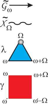
Figure 1: Basic building blocks for dual-boson diagram: fermionic ($\tilde{\mathcal{G}}$) and bosonic ($\tilde{\mathcal{X}}$) dual propagators as well as $\lambda$ and $\gamma$ vertices.

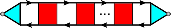
Figure 2: The bosonic dual self-energy in the ladder approximation. A triangle represents the $\lambda$ vertex and a square represents the $\gamma$ vertex

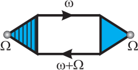
Figure 3: The bosonic dual self-energy with the renormalized triangle vertex.

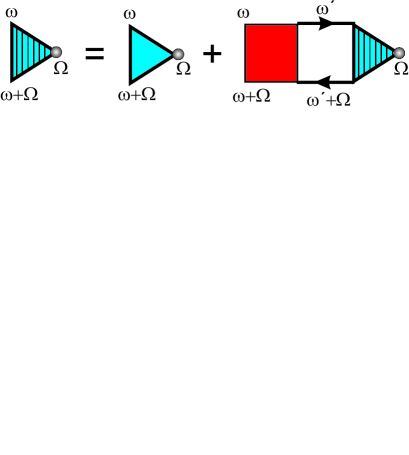
Figure 4: The diagrammatic equation for the renormalized triangle vertex.

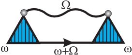
Figure 5: An example of diagram for the fermionic dual self-energy with the renormalized triangle vertex.

References

- [1] T. Moriya, Spin Fluctuations in Itinerant Electron Magnetism, Springer Verlag, Berlin, 1985.
- [2] I. E. Dzyaloshinskii, P. S. Kondratenko, Sov. Phys. JETP 43 (1976) 1036.
- [3] S. V. Vonsovsky, M. I. Katsnelson, A. V. Trefilov, Phys. Metal. Metallography 76 (1993) 247.
- [4] S. V. Vonsovsky, M. I. Katsnelson, A. V. Trefilov, Phys. Metal. Metallography 76 (1993) 343.
- [5] A. I. Lichtenstein, M. I. Katsnelson, G. Kotliar, Phys. Rev. Lett. 87 (2001) 067205.
- [6] A. Georges, G. Kotliar, W. Krauth, M. J. Rozenberg, Rev. Mod. Phys. 68 (1996) 13.
- [7] E. Gull, A. J. Millis, A. I. Lichtenstein, A. N. Rubtsov, M. Troyer, P. Werner, Rev. Mod. Phys. 83 (2011) 349.
- [8] E. Gorelov, J. Kolorenč, T. Wehling, H. Hafermann, A. B. Shick, A. N. Rubtsov, A. Landa, A. K. McMahan, V. I. Anisimov, M. I. Katsnelson, A. I. Lichtenstein, Phys. Rev. B 82 (2010) 085117.
- [9] E. Gorelov, T. O. Wehling, A. N. Rubtsov, M. I. Katsnelson, A. I. Lichtenstein, Phys. Rev. B 80 (2009) 155132.
- [10] G. Kotliar, S. Y. Savrasov, K. Haule, V. S. Oudovenko, O. Parcollet, C. A. Marianetti, Rev. Mod. Phys. 78 (2006) 865.
- [11] A. I. Lichtenstein, M. I. Katsnelson, Phys. Rev. B 57 (1998) 6884.
- [12] M. I. Katsnelson, V. Y. Irkhin, L. Chioncel, A. I. Lichtenstein, R. A. de Groot, Rev. Mod. Phys. 80 (2008) 315.
- [13] R. Chitra, G. Kotliar, Phys. Rev. B 63 (2001) 115110.
- [14] P. Sun, G. Kotliar, Phys. Rev. B 66 (2002) 085120.
- [15] M. I. Katsnelson, A. I. Lichtenstein, J. Phys.: Condens. Mat. (2010) 382201.
- [16] S. Biermann, F. Aryasetiawan, A. Georges, Phys. Rev. Lett. 90 (2003) 086402.
- [17] S. Sachdev, Quantum Phase Transitions, Cambridge University Press, Cambridge, 1999.
- [18] A. A. Abrikosov, L. P. Gorkov, I. E. Dzyaloshinskii, Methods of Quantum Field Theory in Statistical Physics, Pergamon Press, New York, 1965.
- [19] G. G. Mahan, Many-Particle Physics, Plenum Publisher, New York, 2000
- [20] M. Gell-Mann and K. A. Brueckner, Phys. Rev. 106 (1957) 364.
- [21] V. M. Galitskii, Sov. Phys. JETP 7 (1958) 104.
- [22] S. T. Beliaev, Sov. Phys. JETP 7 (1958) 286.
- [23] K. G. Wilson and J. Kogut, Phys. Rep. 12 (1974) 75.
- [24] N. E. Bickers, Rev. Mod. Phys. 59 (1987) 845.
- [25] A. Shiller and K. Ingersent, Phys. Rev. Lett. 75 (1995) 113.
- [26] A. N. Rubtsov, M. I. Katsnelson, A. I. Lichtenstein, Phys. Rev. B 77 (2008) 033101.
- [27] A. N. Rubtsov, M. I. Katsnelson, A. I. Lichtenstein, A. Georges, Phys. Rev. B 79 (2009) 045133.
- [28] H. Hafermann, G. Li, A. N. Rubtsov, M. I. Katsnelson, A. I. Lichtenstein, H. Monien, Phys. Rev. Lett. 102 (2009) 206401.
- [29] G. Kotliar, A. E. Ruckenstein, Phys. Rev. Lett. 57 (1986) 1362.
- [30] D. Bohm, D. Pines, Phys. Rev. 92 (1953) 609.
- [31] V. A. Khodel, V. R. Shaginyan, V. V. Khodel, Phys. Rep. 249 (1994) 1.
- [32] V. Yu. Irkhin, A. A. Katanin, M. I. Katsnelson, Phys. Rev. B 64 (2001) 165107.
- [33] S. Pairault, D. Sénéchal, A.-M. S. Tremblay, Phys. Rev. Lett. 80 (1998) 5389.
- [34] S. Pairault, D. Sénéchal, A.-M. S. Tremblay, Phys. Rev. Lett. 80 (1998) 5389.
- [35] A. N. Rubtsov, Phys. Rev. B 66 (2002) 052107.
- [36] G. Baym, Phys. Rev. 127 (1962) 1391.
- [37] G. Baym, In: Progress in Nonequilibrium Green’s Functions, ed. by M. Bonitz, World Scientific (2000) p. 17.
- [38] J. A. Hertz and D. M. Edwards, J. Phys. F: Metal Phys. 3 (1973) 2173.
- [39] G. Onida, L. Reining, A. Rubio, Rev. Mod. Phys. 74 (2002) 601.
- [40] H. Hafermann, C. Jung, S. Brener, M. I. Katsnelson, A. N. Rubtsov, A. I. Lichtenstein, Europhys. Lett. 85 (2009) 27007.
- [41] A. I. Liechtenstein, M. I. Katsnelson, V. P. Antropov, V. A. Gubanov, J. Magn. Magn. Mater. 67 (1987) 65.
- [42] M. I. Katsnelson, A. I. Lichtenstein, J. Phys.: Condens. Mat. 16 (2004) 7439.
- [43] V. Yu. Irkhin, Yu. P. Irkhin, Phys. Stat. Sol. (b) 183 (1994) 9.
- [44] B. L. Altshuler, A. G. Aronov, Zh. Eksp. Teor. Fiz. 77 (1979) 2028.
- [45] B. L. Altshuler, A. G. Aronov, P. A. Lee, Phys. Rev. Lett. 44 (1980) 1288.
- [46] A. O. Anokhin, M. I. Katsnelson, Int. J. Mod. Phys. B 10 (1996) 2469.
- [47] S. Florens, Ph.D. thesis, University Pierre and Marie-Curie, Paris, 2003.