Energy-Delay Considerations in Coded
Packet Flows

Abstract

We consider a line of terminals which is connected by packet erasure channels and where random linear network coding is carried out at each node prior to transmission. In particular, we address an online approach in which each terminal has local information to be conveyed to the base station at the end of the line and provide a queueing theoretic analysis of this scenario. First, a genie-aided scenario is considered and the average delay and average transmission energy depending on the link erasure probabilities and the Poisson arrival rates at each node are analyzed. We then assume that all nodes cannot send and receive at the same time. The transmitting nodes in the network send coded data packets before stopping to wait for the receiving nodes to acknowledge the number of degrees of freedom, if any, that are required to decode correctly the information. We analyze this problem for an infinite queue size at the terminals and show that there is an optimal number of coded data packets at each node, in terms of average completion time or transmission energy, to be sent before stopping to listen.

I Introduction

In networks, the transfer of packets from source to destination can be in general modeled as a flow of packets [1, 2]. Such a flow is typically routed through intermediate nodes in which the packets are stored in buffers for subsequent transmission. Further, other flows may join existing flows at intermediate nodes in order to be routed towards the same direction downstream in the network. Of particular interest in these scenarios is the average end-to-end delay of packets associated with a specific flow. At the same time, in many scenarios related to networks with energy-constrained nodes, the average completion energy of conveying a packet from source to destination is required to be as small as possible. Satisfying these constraints is particularly challenging in wireless networks where the physical links between nodes may become unreliable due to noise, interference, and fading due to node mobility, which typically leads to packet erasures.

For such packet-erasure networks, one approach to reliable transmission is to employ random linear network coding [3, 4] over stored packets at each node. In the following we will model packet flows in networks by simple erasure line networks. For such networks, it has been shown in [5, 6] that in-network coding is beneficial compared to a traditional end-to-end forward erasure correction approach, and that the min-cut capacity can be achieved asymptotically. The expected delay for multihop line networks and random linear coding has been characterized in [7], and in [8, 9] a queueing-theoretic analysis of finite buffer effects has been carried out.

In this paper we consider packet flows in two-hop erasure line networks. As a new result we study the practically important case of multiple flows by assuming that both the first and the second node in the line have local information packets with Poisson-distributed arrivals available which are demanded by the receiver. For a related scenario and deterministic channels between the nodes the capacity region has been recently established in [10]. In our work, we address both online and batch-to-batch approaches and provide a queueing-theoretic analysis, where average delay and average energy consumption as a function of the link erasure probabilities and the arrival rates at each node are analyzed. We then assume that all terminals cannot send and receive at the same time, which is an extension of the results for the point-to-point case [11, 12] to multihop networks. We show that there is an optimal number of coded data packets at each node, for example in terms of average completion time or energy, to be sent before stopping to listen, and devise an efficient algorithm to find these values. Finally, we compare our half-duplex schemes with selective repeat (i.e., a scheme with no coding).

II Genie-Aided Inter-Session Coding

Let us assume a line network with three nodes, where two adjacent nodes ($S_{1}$, $S_{2}$) are source nodes and the final node is the destination, $R$ (see Fig. 1). Each source $S_{k}$ generates data packets at a rate of $\lambda_{k}$ via a Poisson process; we assume that the packet arrivals at each source are independent from each other. This defines the following packet flows, $S_{1}\rightarrow S_{2}\rightarrow R$ and $S_{2}\rightarrow R$, where flow $k$ is the flow originating at $S_{k}$. We consider an online approach where input packets arrive continuously. Further, our initial system model has normalized slotted time where parallel transmission channels are assumed and thus node $S_{2}$ operates in full-duplex mode. Therefore, at most one packet can be transmitted from $S_{1}$ to $S_{2}$ and at most one from $S_{2}$ to $R$ per slot, where $p_{1}$ and $p_{2}$ are the corresponding erasure probabilities on the links between $S_{1}$ and $S_{2}$ and $S_{2}$ and $R$, respectively. Thus, in order to ensure stability for the queues we assume that $\lambda_{1}\!<\!1\!-\!p_{1}$ for $S_{1}$ and $\lambda_{1}+\lambda_{2}<1\!-\!p_{2}$ for $S_{2}$. Each source node performs inter-session random linear network coding, where at $S_{2}$ all incoming flows are linearly combined. We also assume that each node in the network has full system knowledge provided by a genie.

As in previous works (see, e.g., [6, 8, 9]) we model the system as a Markov process. A state ${\cal S}=(i_{1},i_{2})$ is defined by $i_{1}$ (or $i_{2}$) which denotes the number of degrees of freedom (dof) at $S_{1}$ (or $S_{2}$) that have not been seen at $S_{2}$ (or $R$). The state variable $i_{k}$ represents the number of (coded) packets in the queue $S_{k}$ because all remaining packets can discarded from the queue [13]. We define $a_{(x_{1},x_{2})}\{b\}$ as the probability of $x_{i}$ packets being generated at $S_{k}$ in $b$ time slots, $k=1,2$. Given independence we obtain $a_{(x_{1},x_{2})}\{b\}=a^{(1)}_{(x_{1})}\{b\}a^{(2)}_{(x_{2})}\{b\}$, where $a^{(i)}_{(x_{i})}\{b\}=\frac{e^{-\lambda_{i}b}{\left(\lambda_{i}b\right)}^{x_{i}}}{x_{i}!}$. Further, let $d_{(y_{1},y_{2})|{\cal S}}\{b_{1},b_{2}\}$ be the probability of $y_{k}$ packets being transmitted successfully from $S_{k}$ conditioned on the current state ${\cal S}$ when $b_{k}$ coded packets, generated from the $i_{k}$ packets in the queue, are transmitted. Since we have parallel transmission channels, $d_{(y_{1},y_{2})|{\cal S}}\{b_{1},b_{2}\}=d_{(y_{1})|i}\{b_{1}\}d_{(y_{2})|j}\{b_{2}\}$, where

$$d_{(y_{k})|x}\{b\}=\\ \begin{cases}1&\text{if }x=0,y_{k}=0,\\ \binom{b}{y_{k}}\left(1-p_{k}\right)^{y_{k}}p_{k}^{b-y_{k}}&\text{if }x>0,y_{k}=0,..,\min(x\!,b\!)-\!1\\ \sum_{m=x}^{b}\binom{b}{m}\left(1-p_{k}\right)^{m}p_{k}^{b-m}&\text{if }x>0,y_{k}=\min(x,b)\\ 0&\text{otherwise.}\end{cases}$$

Herein, $x$ denotes the number of state transitions to reach the zero state.

Let us further define $P(T|{\cal S})=P_{{\cal S}\rightarrow{\cal S}^{\prime}}$ as the transition probability between states ${\cal S}=(i_{1},i_{2})$ and ${\cal S}^{\prime}=(i_{1}^{\prime},i_{2}^{\prime})$. This effect is captured by the probability of the random vector $T=(\Delta_{1},\Delta_{2})$, where $\Delta_{k}=i_{k}^{\prime}-i_{k}$. Thus, the transition probability between states ${\cal S}=(i_{1},i_{2})$ and ${\cal S}^{\prime}=(i_{1}^{\prime},i_{2}^{\prime})$ can be written as

$$P(\Delta_{1},\Delta_{2}|{\cal S})=\\ \sum_{y_{1}\in\{0,1\},y_{2}\in\{0,1\}}a_{(\Delta_{1},\Delta_{2}-f(y_{1},y_{2}))}\{1\}\,d_{(y_{1},y_{2})|{\cal S}}\{1,1\}$$

where

$$f(y_{1},y_{2})=\begin{cases}0&\text{if }y_{2}=0,y_{1}=0,\text{ or if }y_{2}=1,y_{1}=1,\\ -1&\text{if }y_{2}=1,y_{1}=0,\\ 1&\text{if }y_{2}=0,y_{1}=1.\end{cases}$$

After some intermediate steps, $P(\Delta_{1},\Delta_{2}|{\cal S})$ can be written as

$$P(\Delta_{1},\Delta_{2}|{\cal S})=d_{(0)|i_{1}}\{1\}\,a^{(1)}_{(\Delta_{1})}\{1\}\,\mathbf{1}_{\{\Delta_{1}\geq 0\}}\cdot\\ \Big{[}d_{(0)|i_{2}}\{1\}\,a^{(2)}_{(\Delta_{2})}\{1\}\,\mathbf{1}_{\{\Delta_{2}\geq 0\}}+\\ d_{(1)|i_{2}}\{1\}\,a^{(2)}_{(\Delta_{2}+1)}\{1\}\,\mathbf{1}_{\{\Delta_{2}\geq-1\}}\Big{]}+\\ d_{(1)|i_{1}}\{1\}\,a^{(1)}_{(\Delta_{1}+1)}\{1\}\,\mathbf{1}_{\{\Delta_{1}\geq-1\}}\cdot\\ \Big{[}d_{(0)|i_{2}}\{1\}\,a^{(2)}_{(\Delta_{2}-1)}\{1\}\,\mathbf{1}_{\{\Delta_{2}\geq 1\}}+\\ d_{(1)|i_{2}}\{1\}\,a^{(2)}_{(\Delta_{2})}\{1\}\,\mathbf{1}_{\{\Delta_{2}\geq 0\}}\Big{]}$$ (1)

where $\mathbf{1}_{\{s\in S\}}$ denotes the indicator function being one when $s\in S$ and zero otherwise.

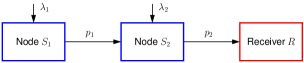
Figure 1: System setup.

II-A Probability Generating Function

In the following, we consider the probability generating function (PGF) for the state transition probabilities $P(T|{\cal S})$. The PGF is useful for computing the steady-state distribution of the underlying Markov process as discussed below. The PGF for a random vector $X=\{x_{1},x_{2},\dots,x_{n}\}$ is defined as

$$M_{X}(Z)=\sum_{K}P(X=K)\prod_{i}z_{i}^{k_{i}}$$ (2)

where $Z=\{z_{1},z_{2},\dots,z_{n}\}$ and $K=\{k_{1},k_{2},\dots,k_{n}\}$. Clearly,

$$\frac{\partial^{k_{1}}}{\partial z_{1}^{k_{1}}}\dots\frac{\partial^{k_{n}}}{\partial z_{n}^{k_{n}}}M_{X}(Z)\Big{|}_{z_{1}=0,\dots,z_{n}=0}\\ =P(x_{1}=k_{1},\dots,x_{n}=k_{n}),$$ (3)

which simplifies the computation of the individual transition probabilities in our approach. For our system we define $M_{T|{\cal S}}(Z)$ as the PGF for the state transition probability when starting in state ${\cal S}$. We have the following lemma.

Lemma 1.

Let $P(T|{\cal S})=P_{{\cal S}\rightarrow{\cal S}^{\prime}}$ be the transition probability between ${\cal S}=(i_{1},i_{2})$ and ${\cal S}^{\prime}=(i_{1}^{\prime},i_{2}^{\prime})$, where $T=(i^{\prime}_{1}-i_{1},i^{\prime}_{2}-i_{2})$. The PGF for the genie-aided case with inter-session coding is given as

$$M_{T|{\cal S}}(z)=e^{\lambda_{1}(z_{1}-1)}e^{\lambda_{2}(z_{2}-1)}\cdot\\ \left(d_{(0)|i_{2}}\{1\}+d_{(1)|i_{2}}\{1\}z_{2}^{-1}\right)\cdot\\ \left(d_{(0)|i_{1}}\{1\}+d_{(1)|i_{1}}\{1\}z_{2}z_{1}^{-1}\right).$$

The proof is omitted due to space constraints.

Positive recurrence of the Markov chain can be shown by using the criteria in [14], which guarantees existence of a unique stationary probability. Let us then define $\pi_{(m,l)}$ as the stationary probability of state $(m,l)$. Using the fact that

$$\pi_{(m,l)}=\sum_{m^{\prime}\geq 0,l^{\prime}\geq 0}\pi_{(m^{\prime},l^{\prime})}P_{(m^{\prime},l^{\prime})\rightarrow(m,l)}$$ (4)

the PGF for $\pi_{(m,l)}$ can be written as $\Pi(z_{1},z_{2})=\sum_{m\geq 0,l\geq 0}\pi_{(m,l)}M_{T|(m,l)}(Z)$. Given that each node can process at most one packet per time slot, the PGF has only four cases of interest: three of them correspond to one or both queues being empty, and the fourth corresponds to the scenario in which both queues have at least one packet. The latter translates into $M_{T|(1,1)}(Z)=M_{T|(a,b)}(Z)$ for $a\geq 1,b\geq 1$. We exploit this fact to express the $\Pi(z_{1},z_{2})$ as

$$\Pi(z_{1},z_{2})(M_{T|(1,1)}(Z)-z_{1}z_{2})=\\ \sum_{g_{1}+g_{2}\leq 1}\pi_{(g_{1},g_{2})}z_{1}^{g_{1}}z_{2}^{g_{2}}-z_{1}z_{2}\pi_{(0,0)}M_{T|(0,0)}(Z)+\\ z_{1}z_{2}\sum_{g_{1}\geq 1}\pi_{(g_{1},0)}M_{T|(1,0)}(Z)+z_{1}z_{2}\sum_{g_{2}\geq 1}\pi_{(0,g_{2})}M_{T|(0,1)}(Z).$$ (5)

This provides an expression for $\Pi(z_{1},z_{2})$ in terms of its coefficients $\pi_{(0,0)},\pi_{(0,1)},\pi_{(1,0)},\pi_{(1,1)}$. Searching for the roots of $M_{T|(1,1)}(Z)-z_{1}z_{2}$ allows us to find linear equations in terms of the unknown coefficients by evaluating the above expression with the obtained roots. Further, from (4) we obtain directly that $\pi_{(0,0)}=\pi_{(0,0)}P(0,0|(0,0))+\pi_{(0,1)}P(0,-1|(0,1))$ and $\pi_{(1,0)}=\pi_{(1,0)}P(0,0|(1,0))+\pi_{(0,1)}P(1,-1|(0,1))+\pi_{(0,0)}P(1,0|(0,0))+\pi_{(1,1)}P(0,-1|(1,1))$, which can be used to determine enough linear equations to solve for the unknown variables $\pi_{(0,0)},\pi_{(0,1)},\pi_{(1,0)},\pi_{(1,1)}$.

II-B Delay

Let us define $D_{k}$ as the time that a packet in $S_{k}$ experiences between being received and being seen at the next hop, and thus discarded from the queue of $S_{k}$. By Little’s Law we obtain

$$E[D_{1}] =\frac{E[i_{1}]}{\lambda_{1}}=\frac{\sum_{m\geq 0}m\big{(}\sum_{l\geq 0}\pi_{(m,l)}\big{)}}{\lambda_{1}},$$ (6)

$$E[D_{2}] =\frac{E[i_{2}]}{\lambda_{2}+\lambda_{1}}=\frac{\sum_{l\geq 0}l\big{(}\sum_{m\geq 0}\pi_{(m,l)}\big{)}}{(\lambda_{1}+\lambda_{2})}.$$ (7)

Note that a packet from flow $1$ will experience an average delay of $E[D_{1}]+E[D_{2}]$ before been see at the end receiver $R$, while a packet from flow $2$ will experience an average delay of $E[D_{2}]$ before being seen at $R$.

II-C Energy

We study the average total energy invested per successfully transmitted packet for each of the two transmitting nodes, $S_{1}$ and $S_{2}$. We consider $E_{k}$ to be the overall energy to convey a packet over a time slot $S_{k}$ (including transmission and reception energy). Each source is considered to operate in cycles, where each cycle has two phases. First, we have an “idle” phase where the queue for $S_{k}$ is empty, which requires $T^{0}_{k}$ time slots. Second, there is a “busy” phase where the queue is not-empty, which requires $T_{k}$ time slots. This constitutes the time the system needs to obtain $i_{k}=0$ for the first time, given that the system starts at $i_{k}>0$ after the reception of packets at the end of the previous idle phase.

Theorem 2.

The average overall energy per transmitted packet at node $S_{k}$, ${\cal E}_{k}$, for the genie-aided case with inter-session coding is given by

$${\cal E}_{1}=(1-P_{em})\,\frac{E_{1}}{\lambda_{1}},\quad{\cal E}_{2}=(1-P_{em})\,\frac{E_{2}}{(\lambda_{1}+\lambda_{2})},$$

where

$$E[T^{0}_{1}]=\frac{1}{1-e^{-\lambda_{1}}},\ E[T^{0}_{2}]=\frac{1}{1-e^{-\lambda_{1}}(P_{em}+p_{1}(1-P_{em}))},$$

and $P_{em}=\frac{E[T^{0}_{1}]}{E[T_{1}]+E[T^{0}_{1}]}$.

Proof.

We present the proof for ${\cal E}_{1}$. The case of ${\cal E}_{2}$ follows naturally. For the genie-aided case, at most one packet can be in the server at any time. When the system is empty, the source will not transmit and no energy is invested in this process. The PASTA-property [15] implies that the probability $P_{em}$ that a packet arrives at an empty system is given by the probability that the system is empty at an arbitrary time. Using a standard argument from renewal theory, the probability of a system being empty is given by the mean idle time divided by the mean cycle time, i.e., $P_{em}=\frac{E[T^{0}_{1}]}{E[T_{1}]+E[T^{0}_{1}]}$. Then, the mean energy per time slot is given by $E_{1}(1-P_{em})$. Dividing this by the arrival rate per time slot $\lambda_{1}$ yields the energy invested for transmissions from $S_{1}$. Since all incoming packets of the first source are due to Poisson arrivals, $E[T^{0}_{1}]=1/(1-e^{-\lambda_{1}})$. For computing $E[T^{0}_{2}]$ it is necessary to consider two sources of incoming packets: the ones which are locally generated and the ones which are received from upstream in the network. Using $P_{em}$, it is clear that $E[T^{0}_{2}]=1/(1-e^{-\lambda_{1}}(P_{em}+p_{1}(1-P_{em})))$. The rest of the proof follows naturally. ∎

III Genie-Aided Intra-Session Coding

In this case we separate both flows by performing random linear coding only within a single flow. Thus, the state representation from Section II needs to be extended by another state variable $i_{3}$. In particular, the new state is defined as ${\cal L}=(i_{1},i_{2},i_{3})$, where $i_{1}$ represents the dof present at $S_{1}$ that have not been seen at $S_{2}$ from flow 1, $i_{2}$ represents the dof present at $S_{2}$ that have not been seen at $R$ from flow 1, and $i_{3}$ represents the dof present at $S_{2}$ that have not been seen at $R$ from flow 2. Since we can only service one packet per time slot and since $S_{2}$ must hence choose one flow for servicing at each time slot, let us first describe the transition probability conditioned on the flow that has been chosen for service. This allows to model different scheduling or resource allocation mechanisms which are implemented at node $S_{2}$ in order to serve both flows.

The probability of transition from state ${\cal L}$ to state ${\cal L}^{\prime}$ is given as ${\cal P}(T|{\cal L})$. We define the event $A_{i}$ as the event of flow $i$ being serviced during the current time slot by node $S_{2}$. Define $\Delta_{k}=i_{k}^{\prime}-i_{k}$. First, let us consider the case in which we condition on flow 1 being serviced, i.e.,

$${\cal P}(T|{\cal L},A_{1})=a^{(2)}_{(\Delta_{3})}\{1\}\left[P(T|{\cal S})|_{\lambda_{2}=0}\right]$$ (8)

where $P(T|{\cal S})|_{\lambda_{2}=0}$ is the state transition probability defined in (1) and evaluated for the case of $\lambda_{2}=0$. If we condition ${\cal P}(T|{\cal L})$ on event $A_{2}$ we obtain

$${\cal P}(T|{\cal L},A_{2})=\Big{(}d_{(1)|i_{3}}\{1\}a^{(2)}_{(\Delta_{3}+1)}\{1\}\mathbf{1}_{\{\Delta_{3}+1\geq 0\}}+\\ d_{(0)|i_{3}}\{1\}a^{(2)}_{(\Delta_{3})}\{1\}\mathbf{1}_{\{\Delta_{3}\geq 0\}}\Big{)}\cdot\\ \Big{(}d_{(1)|i_{1}}\{1\}a^{(1)}_{(\Delta_{1}+1)}\{1\}\mathbf{1}_{\{\Delta_{1}+1\geq 0\}}\mathbf{1}_{\{\Delta_{2}=1\}}+\\ d_{(0)|i_{1}}\{1\}a^{(1)}_{(\Delta_{1})}\{1\}\mathbf{1}_{\{\Delta_{1}\geq 0\}}\mathbf{1}_{\{\Delta_{2}=0\}}\Big{)}.$$ (9)

Note that if node $S_{2}$ implements a policy for choosing the serviced flow in terms of the state, either $A_{1}$ or $A_{2}$ will happen depending on ${\cal L}$. If the system uses a randomized policy, e.g., if it chooses event $A_{1}$ with scheduling probability $P_{s}$ regardless of the starting state ${\cal L}$, then the overall transition probability will be obtained as ${\cal P}(T|{\cal L})=P_{s}{\cal P}(T|{\cal L},A_{1})+(1-P_{s}){\cal P}(T|{\cal L},A_{2})$.

Let us define $D_{k}^{h}$ as the time that a packet in $S_{k}$ from flow $h$ experiences between being received and being seen at the next hop, and thus discarded from the queue of $S_{k}$. We can define the expected delay analogous to Section II-B for the intra-session case. Note that we may devise the policy for servicing flow $1$ and flow $2$ in such a way that $E[D_{1}^{1}]+E[D_{2}^{1}]\approx E[D_{2}^{2}]$, thus providing delay fairness to both flows.

Likewise, similar considerations as in Section II-C for the overall transmission energy also apply in the inter-session case.

IV Half-Duplex Inter-Session Case

We now introduce a half-duplex constraint on the problem in the sense that node $S_{2}$ can only transmit or receive packets, but not both, in a single time slot. We also assume that each node has only access to local information and that ACK packets are employed to update the knowledge about the state of other nodes in the network. ACK packets introduce additional delay and energy consumption. We further assume that $S_{1}$ receives acknowledgments piggybacked in the header of the transmission packets from intended to be sent from $S_{2}$ to $R$.

Let us consider the state $(i_{1},i_{2},S_{t})$, where $i_{1}$ and $i_{2}$ represent the dof missing at node $S_{2}$ and $R$, resp., and $S_{t}$ indicates the node that will be actively transmitting in the upcoming round. We consider that node $S_{1}$ can transmit $N_{i_{1}}$ coded packets in its turn, and that $S_{2}$ can transmit $N_{(i_{1},i_{2})}$ coded packets when it has the opportunity to transmit. We also define a sliding coding window with a maximum number of packets $W_{k}$ that are part of a random linear combination for each node $S_{k}$. Then, the transition probability $(i_{1},i_{2},S_{1})$ to state $(i_{1}^{\prime},i_{2}^{\prime},S_{2})$ can be derived as

$$P(\Delta_{1},\Delta_{2}|(i_{1},i_{2},S_{1}))=\sum_{m=0}^{i_{1}}a({\scriptstyle\Delta_{1}+m})\{{\scriptstyle N_{i_{1}}}\}a({\scriptstyle\Delta_{2}-m})\{{\scriptstyle N_{i_{1}}}\}\cdot\\ \mathbf{1}_{\{\Delta_{2}-m\geq 0\}}\mathbf{1}_{\{\Delta_{1}+m\geq 0\}}d_{(m)|i_{1}}\{N_{i_{1}}\}.$$ (10)

Lemma 3.

Let $P(\Delta_{1},\Delta_{2}|(i_{1},i_{2},S_{1}))$ denote the transition probability between the states $(i_{1},i_{2},S_{1})$ and $(i_{1}^{\prime},i_{2}^{\prime},S_{2})$. The PGF is given as

$$M_{(\Delta_{1},\Delta_{2})|(i_{1},i_{2},S_{1})}(Z)=e^{\lambda_{1}N_{i_{1}}(z_{1}-1)}e^{\lambda_{2}N_{i_{1}}(z_{2}-1)}\cdot\\ \Big{[}\sum_{m=0}^{i_{1}-1}\binom{N_{i_{1}}}{m}\biggl{(}\frac{1-p_{1}}{p_{1}}\biggr{)}^{m}p_{1}^{N_{i_{1}}}z_{1}^{-m}z_{2}^{m}+\\ \sum_{m=i_{1}}^{N_{i_{1}}}\binom{N_{i_{1}}}{m}\biggl{(}\frac{1-p_{1}}{p_{1}}\biggr{)}^{m}p_{1}^{N_{i_{1}}}z_{1}^{-i_{1}}z_{2}^{i_{2}}\Big{]}.$$

The proof is similar to that of Lemma 1 and is also omitted due to space constraints. A similar approach can be followed for the case of transition from state $(i_{1},i_{2},S_{2})$ to state $(i_{1}^{\prime},i_{2}^{\prime},S_{1})$. Finally, we define $T^{(i_{1},i_{2},S_{t})}$ as the time associated to a transition starting at state $(i_{1},i_{2},S_{t})$. As stated in Section II-A for the genie-aided case we can use the PGF in the same way to derive expressions for both expected delay and expected energy consumption.

V Half-Duplex Inter-Session Coding: Batch-by-Batch

Finding the optimal $N_{i_{1}}$ and $N_{(i_{1},i_{2})}$ for the online case discussed in the previous section requires an integer search due to dynamic nature of the online approach. This motivates considering a batch-by-batch approach where the fact that the Markov chain has an absorbing state significantly simplifies the complexity of the optimization problem, as we will describe in the following.

For this case, we model the service process as an absorbing Markov chain with transition probabilities similar to those defined in (10) using $\lambda_{1}=\lambda_{2}=0$. As in the online case, we consider that there is a coding window with a maximum size $M_{k}$ for each node $S_{k}$. The starting state of the Markov chain is given by the number of packets in the queue that are passed to the server, which is limited by the coding window’s maximum size. The absorbing state is constituted by states $(0,0,S_{1})$ and $(0,0,S_{2})$ in Section IV.

We exploit the periodic structure, introduced by the round robin assignment of the transmission in our half-duplex scheme, to estimate $N_{i_{1}}$ and $N_{(i_{1},i_{2})}$. Let us define $T_{(i_{1},i_{2},S_{t})}$ as the mean completion time when the system starts in state $(i_{1},i_{2},S_{t})$. Note that

$$T_{(i_{1},i_{2},S_{1})}=T^{(i_{1},i_{2},S_{1})}+\sum_{i_{1}^{\prime}}P_{(i_{1},i_{2},S_{1})\rightarrow(i_{1}^{\prime},i_{2},S_{2})}T_{(i_{1}^{\prime},i_{2},S_{2})},$$ (11)

$$T_{(i_{1},i_{2},S_{2})}=T^{(i_{1},i_{2},S_{2})}+\sum_{i_{2}^{\prime}}P_{(i_{1},i_{2},S_{2})\rightarrow(i_{1},i_{2}^{\prime},S_{1})}T_{(i_{1},i_{2}^{\prime},S_{1})}.$$ (12)

We can substitute (12) into (11) to obtain

$$T_{(i_{1},i_{2},S_{1})}=T^{(i_{1},i_{2},S_{1})}+\sum_{i_{1}^{\prime}}T^{(i_{1}^{\prime},i_{2},S_{2})}P_{(i_{1},i_{2},S_{1})\rightarrow(i_{1}^{\prime},i_{2},S_{2})}\\ +\sum_{i_{1}^{\prime},i_{2}^{\prime}}\!T_{(i_{1}^{\prime},i_{2}^{\prime},S_{1})}P_{(i_{1},i_{2},S_{1})\rightarrow(i_{1}^{\prime},i_{2},S_{2})}P_{(i_{1}^{\prime},i_{2},S_{2})\rightarrow(i_{1}^{\prime},i_{2}^{\prime},S_{1})}.$$ (13)

This expression captures the fact that node $S_{1}$ can view its communication channel as a transmission link, which has a random waiting time between rounds of transmission. The waiting time depends on the transmissions of node $S_{2}$. We exploit this fact to propose a search algorithm for finding $N_{i_{1}}$ and $N_{(i_{1},i_{2})}$. A similar expression can be found for $T_{(i_{1},i_{2},S_{2})}$ and flow 2 by substituting (11) into (12), and similar expressions hold for the analysis of mean energy with small modifications. For our case, $T^{(i_{1},i_{2},S_{1})}=N_{i_{1}}$ and $T^{(i_{1},i_{2},S_{2})}=N_{(i_{1},i_{2})}+1$. The latter needs to account for a time slot used for transmitting an ACK from $R$ to $S_{2}$.

Let us define $\hat{N}_{i_{1}}(n)$ (or $\hat{N}_{(i_{1},i_{2})}(n)$) as the estimate for $N_{i_{1}}$ (or $N_{(i_{1},i_{2})}$) at step $n$ of the algorithm, and $\hat{P}_{(i_{1},i_{2},S_{1})\rightarrow(i_{1}^{\prime},i_{2},S_{2})}(n)$ and $\hat{P}_{(i_{1},j_{2},S_{1})\rightarrow(i_{1},i_{2}^{\prime},S_{t})}(n)$ are the transition probabilities based on the estimates for the $n$-th step. Finally, we start the algorithm by setting $\hat{N}_{i_{1}}(0)=i_{1}$, $\hat{N}_{(i_{1},i_{2})}(0)=i_{2}$, $n=1$.

Algorithm 1.

S1: TRANSMISSION FROM $S_{1}$ to $S_{2}$:

Compute $\hat{N}_{i_{1}}(n),\forall i_{1}=1,\dots,M_{1}$ to minimize the completion time of a half-duplex link, as in [11], using the waiting time $\sum_{i_{1}^{\prime}}(\hat{N}_{(i_{1}^{\prime},M_{2})}(n)+1)\hat{P}_{(i_{1},M_{2},S_{1})\rightarrow(i_{1}^{\prime},M_{2},S_{2})}$, which corresponds to the second term on the right hand side of (13).

S2: TRANSMISSION FROM $S_{2}$ to $R$:

FOR $i_{1}^{\prime}=1,2,\dots,M_{1}$

Compute $\hat{N}_{(i_{1}^{\prime},i_{2})}(n),\forall i_{2}=1,\dots,M_{2}$ to minimize the completion time of a half-duplex link, as in [11], using the waiting time $\sum_{i_{2}^{\prime}}\hat{N}_{(i_{1}^{\prime},i_{2}^{\prime})}(n)\hat{P}_{(i_{1}^{\prime},i_{2},S_{1})\rightarrow(i_{1}^{\prime},i_{2}^{\prime},S_{1})}(n)$.

STOPPING CRITERIA:

IF $\hat{N}_{(i_{1},i_{2})}(n)=\hat{N}_{(i_{1},i_{2})}(n-1)$, $\forall i,j,t$: STOP

ELSE $n\leftarrow n+1$, and go to S1.

We point out that this search algorithm can be used for both completion time (as shown above) or with different metrics, such as energy or the product of energy and delay to reach a trade-off between both metrics.

VI Numerical Results

Fig. 2 compares genie-aided inter- and intra-session coding by illustrating the delay performance for flows $1$ and $2$, i.e., $E[D_{1}]$ and $E[D_{2}]$ in (6) and (7). For the intra-session case we use a randomized policy at $S_{2}$, which sends packets from flow $1$ with probability $P_{s}$ and services flow $2$ otherwise. For the case of intra-session coding with $P_{s}=0.75$, we observe that the delay for flow $1$ and flow $2$ have the same mean delay performance at $\lambda_{1}=0.12$. As can be seen from Fig. 2 the choice of $P_{s}$ to achieve $E[D_{1}]\approx E[D_{2}]$ depends on the arrival rate. However, this illustrates that the combination of intra-session coding and random scheduling policies at intermediate nodes in a line network can be used successfully to provide delay fairness for sources at different number of hops to the final receiver.

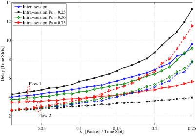
Figure 2: Delay vs arrival rate $\lambda_{1}$ for genie-aided inter- and intra-session coding. Parameters: $\lambda_{2}=0.25$, $p_{1}=0.3$, $p_{2}=0.4$.

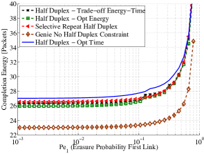
Figure 3: Completion energy in batch-by-batch inter-session coding versus erasure probability. Parameters: $p_{2}=0.4$, $M_{1}=M_{2}=3$ packets, $E_{1}=1$, $E_{2}=2$.

Fig. 3 compares the energy performance for batch-by-batch inter-session coding optimized by using Algorithm 1 for different metrics and for an uncoded selective repeat (ARQ) strategy. Clearly, the completion energy is higher when we optimize for completion time (“Opt. Time”) than optimizing for energy (“Opt. Energy”). If we use a metric that aims to reduce the product of mean energy and and mean time simultaneously (“Trade-off Energy-Time”), it yields an intermediate behavior between the two. The genie case with no half-duplex constraint constitutes a lower bound on energy consumption, because i) it does not require ACK packets, and ii) it sends only enough to complete the transmission.

VII Conclusions

We have considered a two-hop erasure line network where as an extension of existing work each of the first two nodes intents to send local information packets with Poisson-distributed arrivals to the receiver node via random linear network coding. For both online and batch-to-batch schemes a queueing-theoretic framework based on Markov chains and the corresponding moment-generating functions for the state transition probabilities has been provided. We found that despite intra-session random linear coding is not throughput optimal, we can achieve delay fairness for flows coming from different sources by employing a random servicing policy at the middle node in the line network. Then, the half-duplex case is addressed, and it is shown that there is an optimum number of packets each node needs to send before stopping to wait for the receiving nodes to acknowledge the missing degrees of freedom.

References

• [1] L. R. Ford and D. R. Fulkerson, Flows in Networks.   Princeton University Press, 1962.
• [2] R. Ahlswede, N. Cai, S.-Y. R. Li, and R. W. Yeung, “Network information flow,” IEEE Trans. Inf. Theory, vol. 46, no. 4, pp. 1204–1216, Jul. 2000.
• [3] P. Chou, Y. Wu, and K. Jain, “Practical network coding,” in Proc. 41th Allerton Conference on Communication, Control, and Computing, Monticello, IL, Sep. 2003.
• [4] T. Ho, M. Médard, R. Koetter, D. R. Karger, M. Effros, J. Shi, and B. Leong, “A random linear network coding approach to multicast,” IEEE Trans. Inf. Theory, vol. 52, no. 10, pp. 4413–4430, Oct. 2006.
• [5] P. Pakzad, C. Fragouli, and A. Shokrollahi, “Coding schemes for line networks,” in Proc. IEEE Intl. Symp. on Inform. Theory, Adelaide, Australia, Sep. 2005, pp. 1853–1857.
• [6] D. Lun, P. Pakzad, C. Fragouli, M. Medard, and R. Koetter, “An analysis of finite-memory random linear coding on packet streams,” in 4th International Symposium on Modeling and Optimization in Mobile, Ad Hoc and Wireless Networks, Boston, MA, May 2006, pp. 1–6.
• [7] T. K. Dikaliotis, A. G. Dimakis, T. Ho, and M. Effros, “On the delay of network coding over line networks,” in Proc. IEEE Intl. Symp. on Inform. Theory, Seoul, Korea, Jun. 2009, pp. 1408–1412.
• [8] B. N. Vellambi, N. Rahnavard, and F. Fekri, “The effect of finite memory on throughput of wireline packet networks,” in Proc. IEEE Information Theory Workshop, Lake Tahoe, CA, Sep. 2007, pp. 60–65.
• [9] N. Torabkhani, B. N. Vellambi, and F. Fekri, “Study of throughput and latency in finite-buffer coded networks,” in Proc. Asilomar Conference on Signals, Systems, and Computers, Pacific Grove, CA, Nov. 2010.
• [10] T. Lutz, G. Kramer, and C. Hausl, “Capacity for half-duplex line networks with two sources,” in Proc. IEEE Intl. Symp. on Inform. Theory, Austin, TX, Jun. 2010, pp. 2393–2397.
• [11] D. E. Lucani, M. Stojanovic, and M. Médard, “Random linear network coding: When to stop talking and start listening,” in Proc. IEEE INFOCOM, Rio de Janero, Brazil, Apr. 2009, pp. 1800–1808.
• [12] R. N. Swamy and T. Javidi, “Optimal code length for bursty sources with deadlines,” in Proc. IEEE Intl. Symp. on Inform. Theory, Seoul, Korea, Jun. 2009, pp. 2694–2698.
• [13] J. Kumar Sundararajan, D. Shah, and M. Médard, “ARQ for network coding,” in ISIT, 2008, pp. 1651 –1655.
• [14] Z. Rosberg, “A positive recurrence criterion associated with multidimensional queueing processes,” Jour. of Applied Prob., vol. 17, no. 3, pp. 790–801, 1980.
• [15] R. Wolff, “Poisson arrivals see time averages,” Operations Research, vol. 30, no. 2, pp. 223–231, 1982.