Scaling behavior and phase diagram of a $\mathcal{PT}$-symmetric non-Hermitian Bose-Hubbard system

Abstract

We study scaling behavior and phase diagram of a $\mathcal{PT}$-symmetric non-Hermitian Bose-Hubbard model. In the free interaction case, using both analytical and numerical approaches, the metric operator for many-particle is constructed. The derived properties of the metric operator, similarity matrix and equivalent Hamiltonian reflect the fact that all the matrix elements change dramatically with diverging derivatives near the exceptional point. In the nonzero interaction case, it is found that even small on-site interaction can break the $\mathcal{PT}$ symmetry drastically. It is demonstrated that the scaling law can be established for the exceptional point in both small and large interaction limit. Based on perturbation and numerical methods, we also find that the phase diagram shows rich structure: there exist multiple regions of unbroken $\mathcal{PT}$ symmetry.

1 Introduction

Non-Hermitian Hamiltonian is traditionally used to describe open system phenomenologically. It has profound applications in nuclear physics, quantum transport, quantum chemistry, as well as in quantum optics [1]. Since the discovery of a parity-time ($\mathcal{PT}$) symmetric non-Hermitian Hamiltonian can still have an entirely real spectrum, extensive efforts were paid to the pseudo-Hermitian quantum theory [2, 3, 4, 5, 6, 7, 8, 9, 10, 11, 12, 13, 14, 15, 16, 17, 18, 19, 20, 21, 22, 23, 24, 25], which paved the way to our understanding of the connection between non-Hermitian systems and the real physical world. In general, a $\mathcal{PT}$-symmetric non-Hermitian Hamiltonian has unbroken as well as broken $\mathcal{PT}$-symmetric phases, the phase boundary is referred to as the exceptional points (EPs). Studies of the EPs were presented theoretically and experimentally over a decade ago [7, 8, 9]. Recently, the experimental realization of $\mathcal{PT}$-symmetric systems in optics were suggested through creating a medium with alternating regions of gain and loss [20, 21, 22], in which the complex refractive index satisfies the condition $V\left(x\right)=V^{\ast}\left(-x\right)$ and $\mathcal{PT}$ symmetry breaking was observed [23].

One of the characteristic features of the $\mathcal{PT}$-symmetric system is the ubiquitous phase diagram which depicts the symmetry of the eigenfunctions and the reality of the spectrum [11]. The phase separation arises from the fact that although $H$ and the $\mathcal{PT}$ operator commute, the eigenstates of $H$ may or may not be eigenstates of the $\mathcal{PT}$ operator, since the $\mathcal{PT}$ operator is not linear. In the broken $\mathcal{PT}$-symmetric phase the spectrum becomes partially or completely complex, while in the unbroken $\mathcal{PT}$-symmetric phase both $H$ and $\mathcal{PT}$ share the same set of eigenvectors and the spectrum is entirely real. Recently, the phase diagram of a lattice model has been investigated. It is shown that the critical point is sensitive to the distribution of the coupling constant and on-site potential [26, 27, 28, 29].

In this paper, we investigate the effect of on-site interaction on the phase boundary of a $\mathcal{PT}$-symmetric Bose-Hubbard system. Our approach is based on our previous work in Ref. [24], where we have systematically investigated an $N$-site tight-binding chain with a pair of conjugate imaginary potentials $\pm i\gamma$ located at edges. Here we will generalize this description by considering many-particle system and adding the on-site Hubbard interaction $U$. In the free interaction case, many-particle eigenstates are obtained in aid of the single-particle solutions. We also construct the metric operator to investigate the Hermitian counterpart and observables in the framework of complex quantum mechanics. In nonzero $U$ case, we restrict our attention to the influence of the nonlinear on-site interaction $U$ on the boundary between unbroken and broken $\mathcal{PT}$-symmetric phases. Exact Bethe ansatz solution and numerical results show that small on-site interaction can reduce the critical point $\gamma_{c}$ drastically. Moreover, numerical results show that there exist multiple regions of unbroken $\mathcal{PT}$ symmetry and the number of such regions increases as the system size $N$ increases.

This paper is organized as follows. Section 2 describes the Hamiltonian of a $\mathcal{PT}$-symmetric Bose-Hubbard model. In Section 3, we focus on the interaction-free case. Based on the single-particle solutions, we construct the many-particle eigenstates and metric operator to study the Hermitian counterpart and observables. Section 4 is devoted to the case of nonzero interaction. Based on the approximation solutions, we investigate the critical scaling behavior and the phase diagram. Our findings are briefly summarized and the physical relevance of the model and results are discussed in Section 5.

2 $\mathcal{PT}$-Symmetric Bose-Hubbard model

The Bose-Hubbard model gives an approximate description of the physics of interacting bosons on a lattice. Since it embodies essential features of ultracold atoms in optical lattices, the Bose-Hubbard model plays an important role in quantum many-body physics [30, 31]. Optical realization of two-site Bose-Hubbard model in coupled cavity arrays and waveguides have been proposed [32, 33, 34]. It is worth noting that non-Hermitian Bose-Hubbard dimer has attracted enormous research attention in recent years [35, 36, 37, 38, 39, 40]. Theoretical investigations on two site open Bose-Hubbard system was firstly presented in [35]. For a $\mathcal{PT}$-symmetric non-Hermitian Bose-Hubbard dimer, the spectrum and the exceptional points were studied in [36]. After that, dynamics in a leaking double well trap described by non-Hermitian Bose-Hubbard Hamiltonian with additional decay term was investigated under the mean field approximation [37]. Through dynamical study of Bose-Einstein condensed gases, it was shown that imaginary periodic potential may induce perfect quantum coherence between two different condensates [39]. The realization of such open system can be put into practice as a BEC in a double well trap, where the condensate could escape from the traps via tunneling. Most investigations mainly focus on the Bose-Hubbard model with effective decay term in one site.However, it should be noticed that non-Hermitian Bose-Hubbard dimer with complex coupling terms has also attracted some attention, the decay of quantum states could be controlled by modulating the particle-particle interaction strength and the dissipation in the tunneling process [40]. On the other hand, the Bose-Hubbard model with particle loss was investigated in an alternative way through employing Lindblad master equation [41], which phenomenologically describes non-unitary evolution of an open system [42]. Recently, $\mathcal{PT}$-symmetric quantum Liouvillean dynamics is also investigated [43]. In this paper, we investigate the property of a non-Hermitian Hamiltonian in the framework of quantum mechanics.

Nevertheless, although there have been no experiments to show clearly and definitively that a finite non-Hermitian Hamiltonian do exist in nature, many interesting features have been observed in non-Hermitian optical systems, such as double refraction, power oscillations, nonreciprocal phenomenon, etc. [19, 20, 21, 22]. So far, most contributions to pseudo-Hermitian quantum theory were for the single particle problem. Particularly, a two-mode $\mathcal{PT}$-symmetric non-Hermitian Bose-Hubbard system with an imaginary potential on the edge has been investigated [36]. In this paper, we focus on the influence of on-site Hubbard interaction, not restricted to a dimer but to two-particle problem of an $N$-site Bose-Hubbard system. We mainly study the $\mathcal{PT}$-symmetric non-Hermitian Bose-Hubbard system. The Hamiltonian reads

$$H=-J\sum_{l=1}^{N-1}\left(a_{l}^{{\dagger}}a_{l+1}+\text{{H.c.}}\right)+\frac{U}{2}\sum_{l=1}^{N}a_{l}^{{\dagger}2}a_{l}^{2}+i\gamma\left(n_{1}-n_{N}\right)$$ (1)

where $a_{l}^{{\dagger}}$ is the creation operator of the boson at the $l$th site and the tunneling strength is denoted by $J$. The on-site interaction strength and the on-site potential are denoted by $U$ and $i\gamma$, respectively. $H$ is a $\mathcal{PT}$-symmetric Hamiltonian, i.e., $[\mathcal{PT},H]=0$, where the action of the parity operator $\mathcal{P}$ is defined by $\mathcal{P}:l\rightarrow N+1-l$ and the time-reversal operator $\mathcal{T}$ by $\mathcal{T}:i\rightarrow-i$. Both single-particle solution and the critical point $\gamma_{c}$ for interaction-free Hamiltonian $H^{\text{{free}}}=H(U=0)$ have been obtained explicitly in our previous study [24]. The main goal of the present work is to study the influence of the nonlinear interaction on the features of the system.

3 Interaction-free system

When dealing with a $\mathcal{PT}$-symmetric non-Hermitian system, to our knowledge, most researchers concerned about the single-particle problem, since it is believed that the extension of this study to a many-body problem is straightforward. Nevertheless, due to the particular formalism of non-Hermitian quantum mechanics, it is worthwhile to investigate the many-particle system with $U=0$. In the following, we will extend the obtained results for single particle to the case of many-particle system with zero $U$.

3.1 Many-particle solutions

In a non-Hermitian system, although the particle probability is no long conservative, the particle number

$$\hat{N}_{p}=\sum_{l=1}^{N}a_{l}^{{\dagger}}a_{l}$$ (2)

still shares the common eigenfunctions with the Hamiltonian due to the commutation relation

$$[\hat{N}_{p},H^{\text{{free}}}]=[\hat{N}_{p},H]=0.$$ (3)

This fact indicates that the proper inner product should accord with the conservation of particle number. Therefore the eigenstates of $H^{\text{{free}}}$ or $H$ can be obtained in each invariant subspace $V^{N_{p}}$, which is spanned by the occupation number basis

$$\left|n_{1},n_{2},...,n_{N}\right\rangle\equiv\prod_{i=1}^{N}\left|n_{i}\right\rangle,$$ (4)

with $\hat{N}_{p}=\sum_{l=1}^{N}\hat{n}_{l}$, where $\left|n_{l}\right\rangle\equiv(a_{l}^{{\dagger}})^{n_{l}}/\sqrt{n_{l}!}\left|\text{vac}\right\rangle$. Notice that $\left\{\left|n_{1},n_{2},...,n_{N}\right\rangle\right\}$ is orthonormal set under the Dirac inner product. According to our previous work [24], the single-particle solutions $\{\left|\phi_{+}^{k}\right\rangle\}$ and $\{\left|\phi_{-}^{k}\right\rangle\}$, which are eigenfunctions of the systems $H^{\text{{free}}}$ and $(H^{\text{{free}}})^{{\dagger}}$, i.e. $\left|\phi_{+}^{k}\right\rangle=\sum_{l}f_{k}^{l}a_{l}^{\dagger}\left|\text{vac}\right\rangle$, $\left|\phi_{-}^{k}\right\rangle=\sum_{l}g_{k}^{l}a_{l}^{\dagger}\left|\text{vac}\right\rangle$. They can construct the biorthogonal basis set, i.e.,

$$\sum_{l}f_{k}^{l}(g_{k^{\prime}}^{l})^{\ast} =\delta_{kk^{\prime}},$$ (5)

$$\sum_{k}f_{k}^{l}(g_{k}^{l^{\prime}})^{\ast} =\delta_{ll^{\prime}},$$

here $f_{k}^{l}=\phi_{+}^{k}\left(l\right)$, $g_{k}^{l}=\phi_{-}^{k}\left(l\right)$ have the form

$$\phi_{\pm}^{k}\left(l\right)=\frac{e^{ik\left(l-N_{0}\right)}-\xi_{\pm}e^{-ik\left(l+N_{0}\right)}}{\left|\sqrt{\left[1+\left|\xi_{\pm}\right|^{2}\right]\sin\left(Nk\right)/\sin k-2N\xi_{\pm}e^{-ik\left(N+1\right)}}\right|},$$ (6)

where

$$\xi_{\pm}\left(k\right)=\frac{\gamma e^{ik}\mp iJ}{\gamma e^{-ik}\mp iJ}$$ (7)

and $N_{0}=\left(N+1\right)/2$. The symmetries of the wavefunctions and the spectrum reveal that there are two phases, unbroken and broken phase, which are separated by the critical point $\gamma_{c}$,

$$\gamma_{c}=\left\{\begin{array}[]{l}\pm J\text{, }N=2n\\ \pm J\sqrt{\frac{n+1}{n}}\text{, }N=2n+1\end{array}\right.,$$ (8)

where $n=1,2,...$ In the unbroken region with $\left|\gamma\right|<\left|\gamma_{c}\right|$, all the solutions possess $\mathcal{PT}$ symmetry

$$\mathcal{PT}f_{k}^{l}=\left(f_{k}^{N+1-l}\right)^{\ast}=f_{k}^{l},$$ (9)

and the spectrum is entirely real. In the following, we will demonstrate that the above analysis can be extended to many-particle sector. Actually, one can define the operators in $k$ space in the form of

$$\bar{a}_{k} =\sum_{l}f_{k}^{l}a_{l}^{\dagger},$$ (10)

$$a_{k} =\sum_{l}\left(g_{k}^{l}\right)^{\ast}a_{l},$$

which obey the standard bosonic commutation relations

$$\left[a_{k},\bar{a}_{k^{\prime}}\right] =\delta_{kk^{\prime}},$$ (11)

$$\left[a_{k},a_{k^{\prime}}\right] =\left[\bar{a}_{k},\bar{a}_{k^{\prime}}\right]=0.$$

Then the Hamiltonian $H^{\text{{free}}}$ can be written as the diagonal form

$$H^{\text{{free}}}=\sum_{k}\epsilon_{k}\bar{a}_{k}a_{k},$$ (12)

where $\epsilon_{k}=-2J\cos k$ is real. With respect to the canonical commutation relations of (11), the Hamiltonian in the form of (6) can be regarded as the term of the so-called second quantization representation. Defining the occupation number state in $k$-space as

$$\overline{\left|n_{k_{i}}\right\rangle}\equiv\frac{\left(\bar{a}_{k_{i}}\right)^{n_{k_{i}}}}{\sqrt{n_{k_{i}}!}}\left|\text{vac}\right\rangle,$$ (13)

$$\left|n_{k_{i}}\right\rangle\equiv\frac{(a_{k_{i}}^{{\dagger}})^{n_{k_{i}}}}{\sqrt{n_{k_{i}}!}}\left|\text{vac}\right\rangle,$$

which satisfy

$$\bar{a}_{k_{i}}\overline{\left|n_{k_{i}}\right\rangle} =\sqrt{n_{k_{i}}+1}\overline{\left|n_{k_{i}}+1\right\rangle},$$ (14)

$$a_{k_{i}}\overline{\left|n_{k_{i}}\right\rangle} =\sqrt{n_{k_{i}}}\overline{\left|n_{k_{i}}-1\right\rangle},$$

$$a_{k_{i}}^{{\dagger}}\left|n_{k_{i}}\right\rangle =\sqrt{n_{k_{i}}+1}\left|n_{k_{i}}+1\right\rangle,$$

$$\bar{a}_{k_{i}}^{{\dagger}}\left|n_{k_{i}}\right\rangle =\sqrt{n_{k_{i}}}\left|n_{k_{i}}-1\right\rangle.$$

Then, the eigenstates in the subspace $V^{N_{p}}$ of $H^{\text{{free}}}$ and $(H^{\text{{free}}})^{{\dagger}}$ read

$$\overline{\left|n_{k_{1}},n_{k_{2}},...,n_{k_{N}}\right\rangle} \equiv\prod\limits_{i=1}^{N}\overline{\left|n_{k_{i}}\right\rangle},$$ (15)

$$\left|n_{k_{1}},n_{k_{2}},...,n_{k_{N}}\right\rangle \equiv\prod\limits_{i=1}^{N}\left|n_{k_{i}}\right\rangle,$$

respectively. They correspond to the same eigenvale as

$$E\left(n_{k_{1}},n_{k_{2}},...,n_{k_{N}}\right)=\sum_{l=1}^{N}n_{k_{l}}\epsilon_{k_{l}}.$$ (16)

and the total particle number as $N_{p}=\sum_{l=1}^{N}n_{k_{i}}$. Equivalently, we have

$$H^{\text{{free}}}\overline{\left|n_{k_{1}},n_{k_{2}},...,n_{k_{N}}\right\rangle} = E\left(n_{k_{1}},n_{k_{2}},...,n_{k_{N}}\right)\overline{\left|n_{k_{1}},n_{k_{2}},...,n_{k_{N}}\right\rangle},$$ (17)

$$\left(H^{\text{{free}}}\right)^{{\dagger}}\left|n_{k_{1}},n_{k_{2}},...,n_{k_{N}}\right\rangle = E\left(n_{k_{1}},n_{k_{2}},...,n_{k_{N}}\right)\left|n_{k_{1}},n_{k_{2}},...,n_{k_{N}}\right\rangle.$$ (18)

Thus we conclude that for many-particle case, the phase boundary is still at $\gamma_{c}$. Notice that the eigenstates $\{\overline{\left|n_{k_{1}},n_{k_{2}},...,n_{k_{N}}\right\rangle}\}$, $\left\{\left|n_{k_{1}},n_{k_{2}},...,n_{k_{N}}\right\rangle\right\}$ construct a biorthogonal set instead of the set $\left\{\left|n_{1},n_{2},...,n_{N}\right\rangle\right\}$ under the Dirac inner product.

3.2 Metric and Hermitian counterpart

Table 1: The matrix representation of the metric operator $\eta$, similarity matrix $\rho$, and the equivalent Hermitian Hamiltonian $h$ for systems with $N=2,$ $3,$ and $4$ are listed. Here we denote $\lambda=\sqrt{J^{2}-\gamma^{2}},$ $\varsigma_{\pm}=\sqrt{J\pm\gamma},$ and $\tau=\sqrt{J^{2}-\gamma^{2}/2}$. These matrices satisfy the relations (22). The analytical expression for the cases of $N=2,3$ and the numerical plot in Fig. 1 for the case of $N=4$ show that the derivatives of all the matrix elements with respect to $\gamma$ diverge at the exceptional points.

$N$	$2$	$3$	$4$
$\gamma_{c}$	$1$	$\sqrt{2}$	$1$
$H$	$\left(\begin{array}[]{cc}i\gamma&-J\\ -J&-i\gamma\end{array}\right)$	$\left(\begin{array}[]{ccc}i\gamma&-J&0\\ -J&0&-J\\ 0&-J&-i\gamma\end{array}\right)$	$\left(\begin{array}[]{cccc}i\gamma&-J&0&0\\ -J&0&-J&0\\ 0&-J&0&-J\\ 0&0&-J&-i\gamma\end{array}\right)$
$\eta$	$\frac{1}{\lambda}\left(\begin{array}[]{cc}J&i\gamma\\ -i\gamma&J\end{array}\right)$	$\frac{1}{\tau^{2}}\left(\begin{array}[]{ccc}J^{2}&i\gamma J&-\gamma^{2}/2\\ -i\gamma J&J^{2}+\gamma^{2}/2&i\gamma J\\ -\gamma^{2}/2&-i\gamma J&J^{2}\end{array}\right)$	$\left(\begin{array}[]{cccc}\alpha&-i\beta&\mu&-i\nu\\ i\beta&\chi&-i\beta&\mu\\ \mu&i\beta&\chi&-i\beta\\ i\nu&\mu&i\beta&a\end{array}\right)$
$\rho$	$\frac{1}{2\sqrt{\lambda}}\left(\begin{array}[]{cc}\varsigma_{+}+\varsigma_{-}&i\varsigma_{+}-i\varsigma_{-}\\ i\varsigma_{-}-i\varsigma_{+}&\varsigma_{+}+\varsigma_{-}\end{array}\right)$	$\frac{1}{2\tau}\left(\begin{array}[]{ccc}\tau+J&i\gamma&\tau-J\\ -i\gamma&2J&i\gamma\\ \tau-J&-i\gamma&\tau+J\end{array}\right)$	$\left(\begin{array}[]{cccc}a&-ib&c&-id\\ ib&r&-is&c\\ c&is&r&-ib\\ id&c&ib&a\end{array}\right)$
$h$	$\left(\begin{array}[]{cc}0&-\lambda\\ -\lambda&0\end{array}\right)$	$\left(\begin{array}[]{ccc}0&-\tau&0\\ -\tau&0&-\tau\\ 0&-\tau&0\end{array}\right)$	$\left(\begin{array}[]{cccc}0&x&0&y\\ x&0&z&0\\ 0&z&0&x\\ y&0&x&0\end{array}\right)$

According to the quasi-Hermitian quantum mechanics, a bounded positive-definite Hermitian operator $\eta$ in each invariant subspace can be constructed [4] via the eigenstates of $(H^{\text{{free}}})^{{\dagger}}$ as

$$\eta=\sum_{\{n_{k_{i}}\}}\left|n_{k_{1}},n_{k_{2}},...,n_{k_{N}}\right\rangle\left\langle n_{k_{1}},n_{k_{2}},...,n_{k_{N}}\right|,$$ (19)

which is called the metric operator to define the biorthogonal inner product. The $\eta$-metric operator inner product leads to a unitary time evolution [4, 11]. Here $\{n_{k_{i}}\}$ denotes all the possible states with $\sum_{k_{i}}n_{k_{i}}=N_{p}$. One can see that the metric operator fulfils

$$\eta H^{\text{{free}}}\eta^{-1}=(H^{\text{{free}}})^{{\dagger}},$$ (20)

and thus can be employed to construct a Hermitian Hamiltonian $h$ that possesses the same spectrum as $H^{\text{{free}}}$. Actually, the matrix representation of $\eta$ based on the orthonormal basis under the Dirac inner product, says (4), shows that it is a Hermitian matrix. Furthermore, let $\rho=\sqrt{\eta}$ be the unique positive-definite square root of $\eta$. Then the Hermitian operator $\rho$ acts as a similarity transformation to map the non-Hermitian Hamiltonian $H^{\text{{free}}}$ onto its equivalent Hermitian counterpart $h$ by

$$h=\rho H\rho^{-1}.$$ (21)

To demonstrate such a procedure we take the small size systems as examples. In the following, we consider the Hamiltonian matrices $H_{N}$ in single-particle subspace for chain systems with $N=2$, $3$, and $4$. We derive the explicit forms of metric operator $\eta$, similarity matrix $\rho$, and Hermitian counterpart $h$ for non-Hermitian Hamiltonian $H_{N}$. The matrices $\eta$, $\rho$, and $h$ for systems $N=2$, $3$ are expressed in analytical forms in Table 1, while the ones for $N=4$ are plotted in Fig. 1. It is noticed that they satisfy the following relations

$$\mathcal{R}\eta\mathcal{R} = \eta^{\ast}=\eta^{-1},$$ (22a)

$$\mathcal{R}\rho\mathcal{R} = \rho^{\ast}=\rho^{-1},$$ (22b)

$$\mathcal{PT}\eta\mathcal{PT} = \eta,\mathcal{PT}\rho\mathcal{PT}=\rho,$$ (22c)

where matrix $$\mathcal{R} \mathcal{R}\left(m,n\right)=\left(-1\right)^{m}\delta_{mn}$$ is defined as .

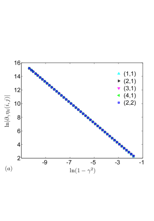
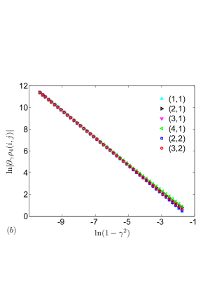
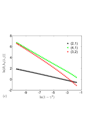
Figure 1: Plots of the derivatives with respect to $\gamma$ of matrix elements of $\eta$ (left panel), $\rho$ (middle panel), and $h$ (right panel) for the case of $N=4$ near the exceptional point $\gamma\rightarrow\gamma_{c}=1$ (taking $J=1$). The numerical results are obtained by exact diagonalization, where $(i,j)$ denotes the index of the matrix elements. It shows that the derivatives of the elements diverge as $\gamma\rightarrow\gamma_{c}$.

All the matrices have the common features: the derivatives of them with respect to $\gamma$ diverge at the exceptional points. This result is not surprising since there is at least a pair of energy levels exhibit repulsion characteristic near $\gamma_{c}$. Nevertheless, we notice that the derivative of the original non-Hermitian Hamiltonian $H^{\text{{free}}}$ is always finite, which reveals the essential difference between a pseudo-Hermitian Hamiltonian and its equivalent Hermitian counterpart. The physics of $h$ near the exceptional point is also obvious: the coupling constants of Hermitian counterpart change dramatically with diverging derivatives.

3.3 Observables

Another theoretical interest in non-Hermitian $\mathcal{PT}$-symmetric system is that the unitary evolution can be obtained by introducing metric operator. In this section, we will illustrate the basic ideas via the above analytical solution.

By introducing $\eta$-metric operator inner product, $\langle\cdot|\cdot\rangle_{\eta}=$ $\left\langle\cdot\right|\eta\left|\cdot\right\rangle$, time evolution can be expressed in a unitary way and also a fully consistent quantum theory can be established [4, 11]. Accordingly, the physical observables $O$ with respect to the metric operator $\eta$ can be constructed to meet the relation [5]

$$\eta O\eta^{-1}=O^{{\dagger}}.$$ (23)

We examine the total particle number operator. It is defined as

$$\hat{N}_{p}=\sum_{l=1}^{N}a_{l}^{\dagger}a_{l}=\sum_{k_{l}}\bar{a}_{k_{l}}a_{k_{l}},$$ (24)

In the invariant subspace $V^{N_{p}}$, we have $[\hat{N}_{p},H^{\text{free}}]=0$, which allows the eigen equations of the operators in the form of

$$\hat{N}_{p}\overline{\left|n_{k_{1}},n_{k_{2}},...,n_{k_{N}}\right\rangle} =N_{p}\overline{\left|n_{k_{1}},n_{k_{2}},...,n_{k_{N}}\right\rangle},$$ (25)

$$\hat{N}_{p}\left|n_{k_{1}},n_{k_{2}},...,n_{k_{N}}\right\rangle =N_{p}\left|n_{k_{1}},n_{k_{2}},...,n_{k_{N}}\right\rangle,$$

and

$$\hat{N}_{p}\left|n_{{}_{1}},n_{{}_{2}},...,n_{{}_{N}}\right\rangle=N_{p}\left|n_{{}_{1}},n_{{}_{2}},...,n_{{}_{N}}\right\rangle.$$ (26)

These indicate that the Hermitian operator $\hat{N}_{p}$ is an observable. Alternatively, this can be proved in the framework of non-Hermitian quantum mechanics. Actually, we have

$$\eta\hat{N}_{p}\eta^{-1} =\sum_{\{n_{k_{i}}\}}|n_{k_{1}},n_{k_{2}},...,n_{k_{N}}\rangle\langle n_{k_{1}},n_{k_{2}},...,n_{k_{N}}|$$ (27)

$$\times\hat{N}_{p}\sum_{\{n_{k_{i}^{\prime}}\}}\overline{|n_{k_{1}^{\prime}},n_{k_{2}^{\prime}},...,n_{k_{N}^{\prime}}\rangle}\overline{\langle n_{k_{1}^{\prime}},n_{k_{2}^{\prime}},...,n_{k_{N}^{\prime}}|}$$

$$=N_{p}\sum_{\{n_{k_{i}}\}}\left|n_{k_{1}},n_{k_{2}},...,n_{k_{N}}\right\rangle\overline{\langle n_{k_{1}},n_{k_{2}},...,n_{k_{N}}|}$$

$$=\hat{N}_{p}^{\dagger}$$

since the biorthogonal basis satisfies

$$\sum_{\{n_{k_{i}}\}}\left|n_{k_{1}},n_{k_{2}},...,n_{k_{N}}\right\rangle\overline{\langle n_{k_{1}},n_{k_{2}},...,n_{k_{N}}|}=1.$$ (28)

Accordingly, for operator $\bar{n}_{k_{l}}=\bar{a}_{k_{l}}a_{k_{l}}$, we also have

$$\eta\bar{n}_{k_{l}}\eta^{-1} =\sum_{\{n_{k_{i}}\}}|n_{k_{1}},n_{k_{2}},...,n_{k_{N}}\rangle\langle n_{k_{1}},n_{k_{2}},...,n_{k_{N}}|$$ (29)

$$\times\bar{n}_{k_{l}}\sum_{\{n_{k_{i}^{\prime}}\}}\overline{|n_{k_{1}^{\prime}},n_{k_{2}^{\prime}},...,n_{k_{N}^{\prime}}\rangle}\overline{\langle n_{k_{1}^{\prime}},n_{k_{2}^{\prime}},...,n_{k_{N}^{\prime}}|}$$

$$=\sum_{\{n_{k_{i}}\}}n_{k_{l}}\left|n_{k_{1}},n_{k_{2}},...,n_{k_{N}}\right\rangle\overline{\langle n_{k_{1}},n_{k_{2}},...,n_{k_{N}}|}$$

$$=\bar{n}_{k_{l}}^{\dagger},$$

in order to obtain (27) and (29) we used (14), (25), and (28).

Then we conclude that the two types of particle number operators, $\hat{N}_{p}=\sum_{l=1}^{N}a_{l}^{\dagger}a_{l}$ and $\bar{n}_{k_{l}}=\bar{a}_{k_{l}}a_{k_{l}}$, are both observables. Besides, the Hamiltonian $H^{\text{{free}}}$ itself and the metric operator $\eta$ are also observables. Here, we would like to clarify that $\hat{N}_{p}$ and $\eta$ are both Hermitian operators, but $H^{\text{{free}}}$ and $\bar{n}_{k_{l}}$ are non-Hermitian operators. However, operators $a_{i}^{\dagger}a_{i}$ and $a_{k_{l}}^{\dagger}a_{k_{l}}$ are no longer observables [4, 10, 13], which are proved through a simple illustration in the A.

Here we want to stress that, the term ”observable” is specific to the non-Hermitian quantum mechanics framework, which differs from that in traditional quantum mechanics. It is still controversial for the interpretation of the observable. As pointed above, $\hat{N}_{p}$ is a good quantum number, or say, the obtained eigenstates of $H$ are also the eigenstates of the total particle number $\hat{N}_{p}$. This guarantees a unitary time evolution if the $\eta$-metric operator inner product is taken. However, the Dirac expectation value of the particle number is not conservative under time evolution, which seems to be expected. This is basically caused by the fact that the eigenstates of $\mathcal{PT}$-symmetric Hamiltonian are non-orthogonal under the Dirac inner product. On the other hand, all Hermitian operators are observables in Hermitian quantum physics. For example, operator $a_{i}^{\dagger}a_{i}$ is an observable in Hermitian quantum mechanics but not regarded as an observable according to the non-Hermitian theory. Nevertheless, it is worth to mention that the observation of the non-Hermitian behavior in experiment, e.g., the power oscillation phenomenon [21][23], is based on the distribution of Dirac expectation value for $a_{i}^{\dagger}a_{i}$.

4 Nonzero interaction system

Now we turn to investigate scaling behavior and phase diagram of the system at nonzero $U$. The boundary of the phase is the main character for a non-Hermitian system. So far most studies dealt with the noninteracting system. For a non-Hermitian lattice model, it is shown that the critical point is sensitive to the distribution of the coupling constant and on-site potential [26, 27, 28]. It indicates that the inhomogeneity of a noninteracting system may shrink the unbroken region of $\mathcal{PT}$ symmetry. From the point of view of mean field theory, on-site interaction takes the role of on-site potentials in some sense. Thus it is presumable that a nonzero $U$ may shift the critical point. In most cases of nonzero $U$, an exact solution is hard to obtain. In this paper, we only consider the two-particle case within some specific parameter areas.

4.1 Solutions for nonzero $U$

The two-particle Bethe ansatz solution

$$\left|\psi_{k_{1},k_{2}}\right\rangle=\sum_{l_{1},l_{2}}f_{k_{1},k_{2}}\left(l_{1},l_{2}\right)a_{l_{1}}^{\dagger}a_{l_{2}}^{\dagger}\left|\text{vac}\right\rangle$$ (30)

where the explicit form of $f_{k_{1},k_{2}}\left(l_{1},l_{2}\right)$ can be expressed as

$$f_{k_{1},k_{2}}\left(l_{1},l_{2}\right)=A\left(k_{1},k_{2}\right)e^{ik_{1}l_{1}+ik_{2}l_{2}}+A\left(k_{2},k_{1}\right)e^{ik_{2}l_{1}+ik_{1}l_{2}}+A\left(k_{1},-k_{2}\right)e^{ik_{1}l_{1}-ik_{2}l_{2}}+A\left(k_{2},-k_{1}\right)e^{ik_{2}l_{1}-ik_{1}l_{2}}$$ (31)

$$+A\left(-k_{1},k_{2}\right)e^{-ik_{1}l_{1}+ik_{2}l_{2}}+A\left(-k_{2},k_{1}\right)e^{-ik_{2}l_{1}+ik_{1}l_{2}}+A\left(-k_{1},-k_{2}\right)e^{-ik_{1}l_{1}-ik_{2}l_{2}}+A\left(-k_{2},-k_{1}\right)e^{-ik_{2}l_{1}-ik_{1}l_{2}}$$

Based on the stationary Schrödinger equation

$$H\left|\psi_{k_{1},k_{2}}\right\rangle=E(k_{1},k_{2})\left|\psi_{k_{1},k_{2}}\right\rangle,$$ (32)

quasimomenta $k_{1}$ and $k_{2}$ satisfy the equations

$$\frac{\left(J^{2}+\gamma^{2}e^{i2k_{1}}\right)e^{-ik_{1}\left(N+1\right)}}{\left(J^{2}+\gamma^{2}e^{-i2k_{1}}\right)e^{ik_{1}\left(N+1\right)}}=\frac{G_{-+}G_{++}}{G_{--}G_{+-}},$$ (33)

$$k_{1}\leftrightarrow k_{2}.$$ (34)

where

$$G_{\sigma\sigma^{\prime}}=2Ji\sin k_{1}+\sigma 2Ji\sin k_{2}+\sigma^{\prime}U$$ (35)

with $\sigma$, $\sigma^{\prime}=\pm$. Hereafter $k_{1}\leftrightarrow k_{2}$ denotes the corresponding equation by exchanging $k_{1}$ and $k_{2}$. The quasimomenta $k_{1}$, $k_{2}$ and amplitudes $A\left(k_{1},k_{2}\right)$ can be determined by (32) and the proper definition of inner product according to the $\mathcal{PT}$-symmetric quantum theory. The corresponding eigenvalue is $E(k_{1},k_{2})=-2J\left(\cos k_{1}+\cos k_{2}\right),$ the reality of $E(k_{1},k_{2})$ determines the phase diagram of the system. It is obvious that (33) and (34) are invariant under $k_{1}\rightarrow k_{2}$, $k_{2}\rightarrow k_{1}$; and also under $k_{1}\rightarrow-k_{1}$, $k_{2}\rightarrow-k_{2}$. We rewritten (33) and (34) explicitly as

$$\begin{array}[]{r}\left(U/J\right)\sin k_{1}\left\{\cos\left[k_{1}\left(N+1\right)\right]+\left(\gamma/J\right)^{2}\cos\left[k_{1}\left(N-1\right)\right]\right\}\\ +\left\{\sin\left[k_{1}\left(N+1\right)\right]+\left(\gamma/J\right)^{2}\sin\left[k_{1}\left(N-1\right)\right]\right\}\\ \times\left[\sin^{2}k_{2}-\sin^{2}k_{1}+\left(U/2J\right)^{2}\right]=0\end{array},$$ (39)

$$k_{1}\leftrightarrow k_{2}.$$ (40)

Although the analytical solutions of (39) and (40) are hard to obtain, approximate solutions within certain ranges of the parameters $\gamma$, $J$, and $U$ may shed light on the influence of $U$ on the phase boundary.

4.2 Solutions at the point $\gamma=J$

We start with the solution of an even $N$ system at the point $\gamma=J$, which is the exceptional point for the system of $U=0$. The influence of on-site interaction on the phase boundary can be qualitatively revealed. Taking $\gamma=J$, (39) and (40) are reduced to

$$U\sin k_{1}\cos\left(k_{1}N\right)+J\left[\left(U/2J\right)^{2}+\cos^{2}k_{1}\right]\times\sin\left(k_{1}N\right)=0,k_{2}=\pi/2,$$ (41)

$$k_{1}\leftrightarrow k_{2}.$$ (42)

respectively. We notice that $k_{1}=\pi/2$ is the solution of (41) for $U=0$. Then for small $U$ case, the solutions should have the form $(\pi/2,\pi/2+\theta_{2})$ and $(\pi/2+\theta_{1},\pi/2)$. For sufficient small $U$, taking the approximations $\sin\left(\theta_{1,2}N\right)\approx\theta_{1,2}N$ and $\cos\left(\theta_{1,2}N\right)\approx 1$, the critical equation reduces to

$$\theta_{1,2}^{3}+\left(U/2J\right)^{2}\theta_{1,2}+U/\left(JN\right)=0$$ (43)

which has one real root and two non-real complex conjugate roots, since the discriminant of the cubic equation $\Delta=\left[U/\left(2JN\right)\right]^{2}$ $+[\left(U/2J\right)^{2}/3]^{3}>0$. Furthermore, one can get the solution of the cubic equation by routine. In order to obtain a concise expression of $\theta_{1,2}$, we simply ignore the term of $U^{2}$ in the cubic equation, and then obtain $\theta_{1,2}=-\sqrt[3]{U/JN}$, $(1\pm i\sqrt{3})\sqrt[3]{U/8JN}$. The corresponding complex conjugate eigenvalues are $E_{\pm}=2J\sin\theta_{1,2}$ $\approx(1\pm i\sqrt{3})\sqrt[3]{UJ^{2}/N}$. Then we can conclude that point $\gamma=J$ is in the broken $\mathcal{PT}$-symmetric region in the presence of on-site interaction, which shrinks the unbroken region of $\mathcal{PT}$ symmetry. Note that for a given $N$, the eigenvalues $E_{\pm}$ become further away from real values as $U$ grows. This agrees with the numerical simulation for phase diagram of the finite size systems.

4.3 Exceptional points and scaling behavior

Now we focus on the phase boundary of the system with small $U$. It is presumable that one pair of coalescing eigenstates have the quasimomenta $k_{1,2}=$ $\pi/2+\delta_{1,2}$ with $\left|\delta_{1,2}\right|\ll 1$. The original critical (39) and (40) are reduced to

$$\begin{array}[]{r}\left(U/J\right)\cos\delta_{1}\left\{\sin\left[\delta_{1}\left(N+1\right)\right]-\left(\gamma/J\right)^{2}\sin\left[\delta_{1}\left(N-1\right)\right]\right\}\\ -\left\{\cos\left[\delta_{1}\left(N+1\right)\right]-\left(\gamma/J\right)^{2}\cos\left[\delta_{1}\left(N-1\right)\right]\right\}\\ \times\left[\cos^{2}\delta_{2}-\cos^{2}\delta_{1}+\left(U/2J\right)^{2}\right]=0\end{array},$$ (47)

$$\delta_{2}\leftrightarrow\delta_{1}.$$ (48)

Furthermore, under the approximation $\left|\delta_{1,2}\right|N\ll 1$ and ignoring the term of $U^{2}$, (39) and (40) are reduced to polynomial equations

$$\left(\delta_{1}^{2}-\delta_{2}^{2}\right)\left(\zeta-\delta_{1}^{2}\right)-\left(N^{2}\zeta+1\right)\delta_{1}u=0,$$ (49)

$$\delta_{2}\leftrightarrow\delta_{1},$$ (50)

where we have defined

$$\zeta N=\frac{J^{2}-\gamma^{2}}{J^{2}+\gamma^{2}},uN=\frac{U}{J}.$$ (51)

Eliminating $\delta_{2}$, one can obtain the equation about $\delta_{1}$ in the form of

$$f\left(\delta_{1}\right)=\delta_{1}^{6}-\zeta\delta_{1}^{4}+u\left(\zeta N^{2}+1\right)\delta_{1}^{3}-\zeta^{2}\delta_{1}^{2}+\zeta^{3}=0,$$ (52)

which solution determines the eigenvalues. As pointed out in Ref. [24], when the eigenstates turn to coalescence at the critical point $\gamma_{c}$, $f\left(\delta_{1}\right)$ should also satisfy the equation d$f\left(\delta_{1}\right)/$d$\delta_{1}=0$. Eliminating $\delta_{1}$ from (52) and d$f\left(\delta_{1}\right)/$d$\delta_{1}=0$, we have

$$3^{3}u^{2}\left(\zeta N^{2}+1\right)^{2}-2^{8}\zeta^{3}=0$$ (53)

under the condition $\left|\zeta\right|N^{2}\ll 1$. Then we can obtain $\gamma_{c}$ approximately as

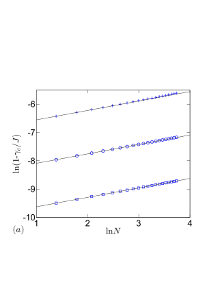
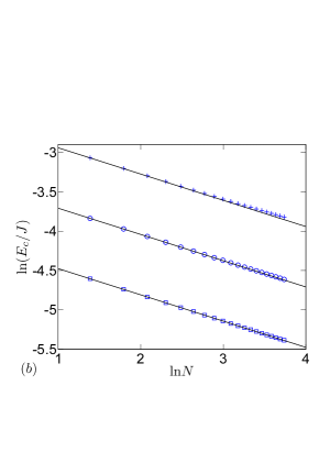
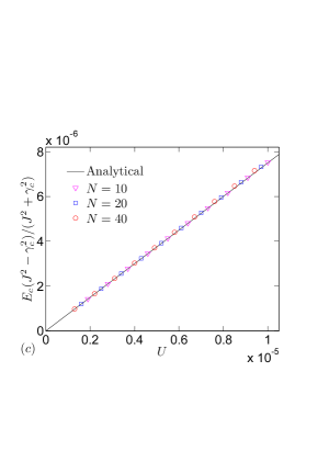
Figure 2: (Color online) Plots of (57), (58), (59) and the corresponding numerical simulation obtained by exact diagonalization. In (a) and (b), the blue crosses, circles and squares indicate the numerical results for the cases of $U=10^{-4}$, $10^{-5}$ and $10^{-6}$, respectively. The black lines are the plots of the corresponding analytical expressions. It shows that they are in agreement with each other for $U=10^{-5}$ and $10^{-6}$. In the case of $U=10^{-4}$, a slight deviation appears for large $N$. From (c), it is observed that the numerical result accords with the analytical expression very well for $N=10$ and $20$. A slight deviation appears for large $U$ in the $N=40$ system.

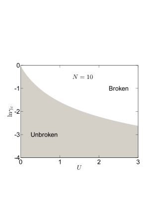
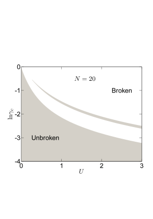
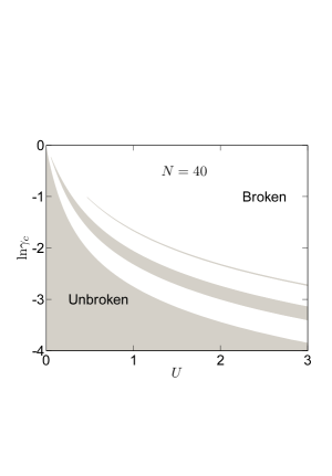
Figure 3: Phase diagrams obtained by exact diagonalization for finite systems with $N=10$, $20$, and $40$. The shadow area indicates the region where the spectrum is entirely real. It shows that as $N$ increases the unbroken $\mathcal{PT}$-symmetric region becomes narrow. There are multiple unbroken $\mathcal{PT}$-symmetric regions appear as $N$ increases.

$$\gamma_{c}=J\sqrt{\frac{1-\beta}{1+\beta}}\simeq J\left(1-\beta\right),$$ (54)

where $\beta=\left(3/8\right)\sqrt[3]{2NU^{2}/J^{2}}$. It shows that the exceptional point exhibits an interaction sensitivity and undergoes dramatic changes following the change of the Hubbard interaction. Substituting $\gamma_{c}$ into (49) and (50), we have

$$\delta_{1,2}=\frac{1\pm i\sqrt{2}}{2}\sqrt[3]{\frac{U}{2JN}},$$ (55)

which leads to the critical eigenvalue

$$E_{c}=2J\left(\sin\delta_{1}+\sin\delta_{2}\right)\approx 2J\sqrt[3]{\frac{U}{2JN}}.$$ (56)

At $U=0$, (54) and (56) reproduce the obtained results in our previous work [24]: $\gamma_{c}=J$ and $E_{c}=0$, respectively. Furthermore, it is observed that for small $U$ and finite $N$, the critical quantities $\gamma_{c}$ and $E_{c}$ can be expressed as

$$\ln\left(1-\gamma_{c}/J\right) \approx \frac{1}{3}\ln N+\ln[\frac{3}{2^{8/3}}\left(\frac{U}{J}\right)^{2/3}],$$ (57)

$$\ln\left(E_{c}/J\right) \approx -\frac{1}{3}\ln N+\ln[2^{2/3}\left(\frac{U}{J}\right)^{1/3}],$$ (58)

which shows the similar dependence on the size of the system. According to the finite-size scaling ansatz [44], the critical behavior can be extracted from the above-mentioned finite samples. Then combining (54) with (56) leads to

$$E_{c}\frac{J^{2}-\gamma_{c}^{2}}{J^{2}+\gamma_{c}^{2}}=\frac{3}{4}U,$$ (59)

which is a universal scaling law for such a phase transition in small $U$ limit. To verify and demonstrate the above analysis, numerical simulations are performed to investigate the scaling behavior. We compute the quantities $\gamma_{c}$ and $E_{c}$ for finite systems, which are plotted in Fig. 2 as comparison with the analytical results (57), (58), and (59). It shows that for small $U$, they are in agreement with each other. It is worthy to note that the analytical expressions in (57), (58), and (59) are obtained under the condition $UN^{2}/J\ll 2^{4}/\sqrt{3^{3}}$ (obtained from $\left|\delta_{1,2}\right|N\ll 1$ and $\left|\zeta\right|N^{2}\ll 1$). Thus for large size system, the scaling law holds only within a very small parameter region. Nevertheless, our finding reveals the fact that there should exist a universal scaling law for such kind of phase transition.

In the interaction-free case, from Section 3 we notice that the $\mathcal{PT}$ symmetry phase hardly changes as the system size $N$ increasing. In contrast, for medium interaction $U$, we investigate the phase diagram for finite size system by numerical simulation. The phase boundary is determined from the reality of the eigenvalues obtained by exact diagonalization. In Fig. 3, the phase diagrams are plotted as $\gamma_{c}$ versus $U$ for finite size chains. It shows that the on-site interaction breaks the $\mathcal{PT}$ symmetry drastically. Interestingly, there exist several $\mathcal{PT}$-symmetric regions and the number of such regions increases as $N$ increases. The phase diagram shows rich structure in cases of medium $U$.

4.4 Phase transition induced by bound-pair state

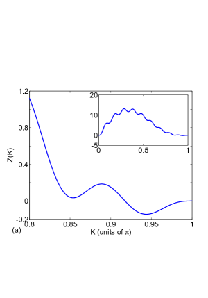
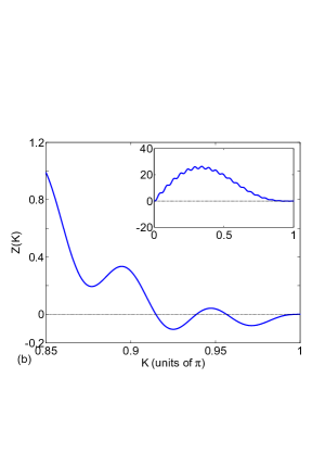
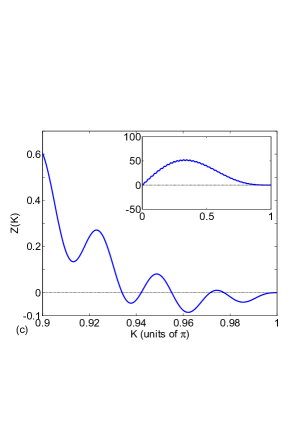
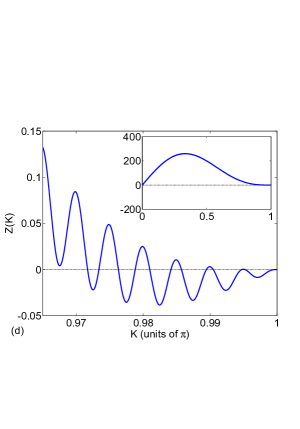
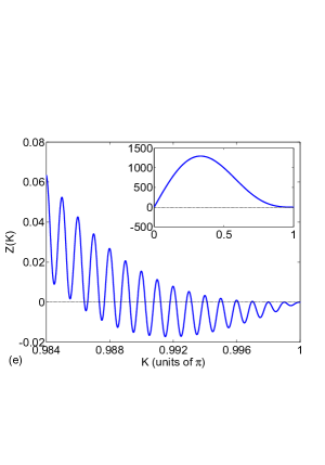
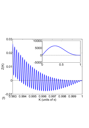
Figure 4: Plots of function $Z\left(K\right)$, insert is $Z\left(K\right)$ in the region $\left(0,\pi\right)$. (a) $N=10$, (b) $N=20$, (c) $N=40$, (d) $N=200$, (e) $N=1000$, (f) $N=5000$. The number of roots of $Z(K)=0$ is $1,3,5,11,27,63$, the number of unbroken $\mathcal{PT}$ symmetric regions is $1,2,3,6,14,32$, respectively. The black line, $Z(K)$ being zero, is a guide to the eye only.

In the following, we analytically investigate the boundaries of the $\mathcal{PT}$-symmetric phase of $H$. In strong on-site interaction case, there exists bound-pair band induced by the interaction $U~{}$[45, 46, 47]. In the presence of $\gamma$, the $\mathcal{PT}$ symmetry is fragile. Here we focus on $\mathcal{PT}$-symmetric breaking phase transition caused by the bound-pair state. We analyse the phase diagram by introducing an effective Hamiltonian $H_{\mathrm{eff}}$, which describes the bound states of system $H$ in strong on-site interaction $U$ region. Based on the perturbation methods [47], the effective Hamiltonian $H_{\mathrm{eff}}$ reads

$$H_{\mathrm{eff}}=\frac{2J^{2}}{U}\left(b_{i}^{\dagger}b_{i+1}+\mathrm{h.c.}\right)+\left(U+\frac{4J^{2}}{U}\right)b_{i}^{\dagger}b_{i}-\frac{2J^{2}}{U}\left(b_{1}^{\dagger}b_{1}+b_{N}^{\dagger}b_{N}\right)+2i\gamma\left(b_{1}^{\dagger}b_{1}-b_{N}^{\dagger}b_{N}\right),$$ (60)

where $b_{i}^{\dagger}=a_{i}^{\dagger 2}/\sqrt{2}$ ($b_{i}=a_{i}^{2}/\sqrt{2}$) is the bound pair creation (annihilation) operator on site $i$.

Similarly as in Section 4, the Hamiltonian $H_{\mathrm{eff}}$ in single-particle invariant subspace can be solved by Bethe ansatz method. We are interested in the bound-pair band, which has the spectrum $E\left(K\right)\approx U+(4J^{2}/U)\left(1+\cos K\right)$. Here, quasimomenta $K$ of the bound-pair state satisfies the equation

$$g\left(K\right)=2(J^{2}/U)^{2}\sin\left(NK\right)\left(1+\cos K\right)+\gamma^{2}\sin\left[\left(N-1\right)K\right]=0.\text{ }$$ (61)

As pointed above, together with the condition $\mathrm{d}g\left(K\right)/\mathrm{d}K=0$, one can obtain the equation

$$Z\left(K\right)=N\left(\cos K+1\right)\sin K-\sin\left(NK\right)\left\{\cos\left(NK\right)+\cos\left[\left(N-1\right)K\right]\right\}=0,\text{ }$$ (62)

which solutions $K_{c}\in\left(0,\pi\right)$ determine the boundaries of quantum phase for the effective Hamiltonian $H_{\mathrm{eff}}$. In other words, function $Z\left(K\right)$ with $\mathcal{N}_{c}$ zeros indicates $\lfloor\mathcal{N}_{c}/2\rfloor+1\$unbroken $\mathcal{PT}$-symmetric regions of both $H_{\mathrm{eff}}$ and $H$, where $\lfloor\mathcal{N}_{c}/2\rfloor$ denotes the integer part of $\mathcal{N}_{c}/2$. To demonstrate this point, function $Z\left(K\right)$ is plotted for different $N$ in Fig. 4. One can see that, the number of solutions $\mathcal{N}_{c}$ increases as $N$ increases, which corresponds to the increasing unbroken $\mathcal{PT}$-symmetric regions. To be specific, for $N=10$, $20$, and $40$, it shows that $\mathcal{N}_{c}=1$, $3$, and $5$, respectively. This indicates there are $1$, $2$, and $3$ unbroken regions, which accords to the phase diagram in Fig. 5. Quantitatively, one can obtain the solutions of $K_{c}$ and $\gamma_{c}$ from (61) for these three cases numerically, which are listed in the following,

$$\begin{tabular}[]{rr}$K_{c}/\pi=$&$0.917579,$\\ $-\ln\gamma_{c}/\ln(J^{2}/U)=$&$1.515811,$\end{tabular}\text{ }(\mathrm{for}\text{ }N=10),$$ (65)

$$\begin{tabular}[]{rrrr}$K_{c}/\pi=$&$0.956567,$&$0.938854,$&$0.914870,$\\ $-\ln\gamma_{c}/\ln(J^{2}/U)=$&$2.124320,$&$1.510840,$&$1.395938,$\end{tabular}\text{ }(\mathrm{for}\text{ }N=20),$$ (68)

$$\begin{tabular}[]{rrrrrr}$K_{c}/\pi=$&$0.977429,$&$0.971547,$&$0.955142,$&$0.942098,$&$0.933982,$\\ $-\ln\gamma_{c}/\ln(J^{2}/U)=$&$2.746955,$&$2.305626,$&$2.041551,$&$1.633456,$&$1.611533.$\end{tabular}\text{ }(\mathrm{for}\text{ }N=40).$$ (71)

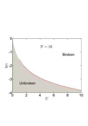
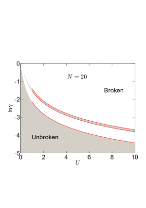
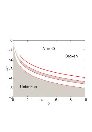
Figure 5: The analytical boundaries (65), (68), (71) (red lines) and the phase diagram in large $U$ region obtained by exact diagonalization for system $H$ of size $N=10,20,40$. The analytical boundaries are plotted in the region of $U=1$ to $10$, where $J$ is set as the unit. It is noticed that the analytical boundaries fit the exact phase diagram well at the large $U$ region.

According to the above analysis, equations (65, 68, 71) represent the phase boundaries, which are plotted as red lines in Fig. 5 as comparison. It shows that the boundaries obtained from equations (65, 68, 71) are in agreement with the exact phase diagram well in large $U$ regime.

For large $N$, the number of unbroken regions can be estimated as the integer around $\sqrt{2N}/\pi$, the analytical results for different $N$ of Fig. 4 is listed in (72) as comparison, it is noticed that the analysis accords with the plots in Fig. 4.

$$\begin{array}[]{ccccccc}N&10&20&40&200&1000&5000\\ \sqrt{2N}/\pi&1.42&2.01&2.85&6.37&14.24&31.83\\ [\sqrt{2N}/\pi]&1&2&3&6&14&32\end{array}.$$ (72)

The ceiling (highest) phase boundary is determined by the root of (62) near $K_{0}\approx\sqrt{2/N}$, correspondingly, the ceiling phase boundary $\gamma_{c}$ is near $\gamma_{0}\approx(J^{2}/U)\sqrt{2/\left(N-1\right)}$.

Now we turn to analyse the floor (lowest) phase boundary for $H_{\mathrm{eff}}$, which corresponds to the solutions $K_{c}$ being in the region $[(N-1)\pi/N,\pi]$. Setting $K=\pi-\left(1-\delta\right)\pi/N$ with $\delta\ll 1$ for large $N$, equation (62) can be reduced to

$$N\left\{1-\cos\left[\left(1-\delta\right)\pi/N\right]\right\}\sin\left[\left(1-\delta\right)\pi/N\right]-\sin\left(\pi\delta\right)\left\{\cos\left(\pi\delta\right)-\cos\left[\pi\delta+\left(1-\delta\right)\pi/N\right]\right\}=0.\text{ }$$ (73)

Moreover, by applying the Taylor expansion, it becomes

$$2\left(N-1\right)\delta^{2}+3\delta-1=0.$$ (74)

Solving this equation, one can obtain $\delta_{c}=(\sqrt{8N+1}-3)/\left(4N-4\right)$, and then the exceptional point $\gamma_{c}$ as

$$\gamma_{c}\approx\frac{J^{2}}{U}\sqrt{\frac{\pi^{2}}{N}\frac{\delta_{c}\left(\delta_{c}-1\right)^{2}}{\left(N-1\right)\delta_{c}+1}}.$$ (75)

We plot the exact and analytical approximation results for the floor phase boundary of $H_{\mathrm{eff}}$, the exact result for the original Hamiltonian $H$ in Fig. 6 as a comparison. The plots fit well, especially at large $U$ case. Remarkably, it also gives a good approximation for those of medium $U$.

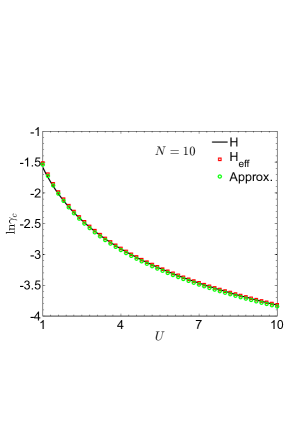
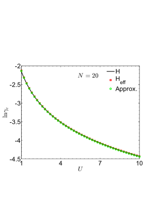
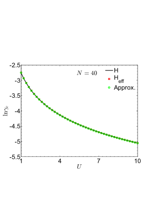
Figure 6: Plots of the floor phase boundary of the phase diagram for $N=10,20,40$. Black solid lines are the exact results obtained from diagonalization of the Bose-Hubbard Hamiltonian $H$. Red squares represent the exact result obtained from the effective Hamiltonian $H_{\mathrm{eff}}$. Green circles are the analytical approximation (75). It is noticed that $H_{\mathrm{eff}}$ and the approximation effectively describe the floor phase boundary of $H$.

It is observed from Fig. 6 that $H_{\mathrm{eff}}$ gives quite good description of the phases of $H$ for system with $U>1$. On the other hand, the critical energy $E_{c}$ can be approximately expressed as

$$E_{c}\approx U+\frac{2J^{2}\pi^{2}}{UN^{2}}\left(1-\delta_{c}\right)^{2}$$ (76)

for large $N$. From the expression (75), (76) of $\gamma_{c}$, $E_{c}$, we have

$$\left(1-\frac{J^{2}}{2U}\frac{E_{c}-U}{\gamma_{c}^{2}}\right)^{2}\approx\frac{2U\gamma_{c}}{J^{2}\pi},$$ (77)

which is a universal scaling law for such a phase transition in large $N$, $U$ case. Numerical simulations are performed to investigate the scaling behavior. We compute the quantities $\gamma_{c}$ and $E_{c}$ for finite systems $H_{\mathrm{eff}}$, which are plotted in Fig. 7 as comparison with the analytical results (75), (76) and (77). It shows for large $N$, they are in agreement with each other.

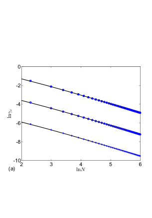
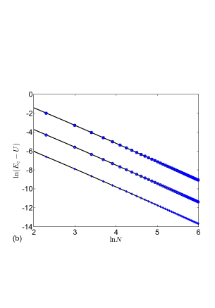
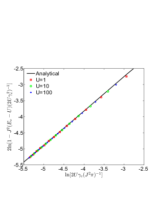
Figure 7: Plots of (75), (76), (77) and the corresponding numerical simulation obtained by exact diagonalization of $H_{\mathrm{eff}}$. $J=1$ is the unit. In (a), (b), the blue squares, circles and crosses indicate the numerical results for the cases of $U=1$, $10$ and $100$, respectively. In (c), the red squares, green circles and blue crosses stand for $U=1$, $10$ and $100$. The black lines are the plots of the corresponding analytical expressions (75), (76), (77). It shows that they are in agreement in large $N$ region.

In the limit $N$ goes to infinity, we notice that $\gamma_{c}=1$ when $U=0$, means that in the region $\gamma<1$, system $H$ is in the unbroken $\mathcal{PT}$-symmetric phase. In non-zero interaction ($U\neq 0$) case, from the above discussions we have the floor phase boundary $\gamma_{c}\approx J^{2}\pi\left(UN\right)^{-1}$ and ceiling phase boundary $\gamma_{0}\approx(J^{2}/U)\sqrt{2/(N-1)}$ for large $N$. As $N$ goes to infinity, it is noticed that $\lim_{N\rightarrow\infty}\left(\gamma_{c}\right)=0$ and $\lim_{N\rightarrow\infty}\left(\gamma_{0}\right)=0$ for non-zero finite $U$. In other words, there always exist bound-pair bound states with conjugate complex energies, which result in the $\mathcal{PT}$-symmetry breaking for non-zero $\gamma$.

System features experience huge changes as system parameter approaching the $\mathcal{PT}$-symmetric phase transition point (exceptional point). Distinguished from phase transition in Hermitian system, the non-analytic properties in $\mathcal{PT}$-symmetric phase transition are caused by the Hamiltonian becoming a Jordan block operator at the exceptional point. Correspondingly, dynamical behavior near the exceptional point experiences dramatic changes, e.g. the power oscillation amplitude becomes significantly large and the corresponding oscillation frequency becomes small. These features could be useful for weak signal detection, or for amplifier design. Phase diagram and the scaling behavior show us rich information where phase transition happens, this maybe helpful for the design and application of quantum devices.

5 Conclusion and discussion

In this paper, we have studied the scaling behavior and phase diagram of a non-Hermitian $\mathcal{PT}$-symmetric Bose-Hubbard model. For interaction-free case, the metric operator is constructed, which is employed to investigate the particle number operator and the corresponding Hermitian counterpart. The derived properties of the metric operator, similarity matrix and equivalent Hamiltonian reflect the fact that they have a common feature: all the matrix elements change dramatically with diverging derivatives near the exceptional point. For nonzero $U$ case, it is found that even small on-site interaction can break the $\mathcal{PT}$ symmetry drastically. It has been demonstrated that the scaling behavior can be established for the exceptional point in both small and large $U$ limit. Based on numerical approach, we find that the phase diagram shows rich structure for medium $U$ and analyse the phase transition boundary. Finally, it is worthwhile to point out that the phase transition discussed differs from the original quantum phase transition in a Hermitian system [49]. The former aims at certain eigenstates of a non-Hermitian Hamiltonian, while the later concerns only the ground state of a Hermitian one. However, our finding reveals that both of them exhibit the scaling behavior, which may be due to they both relate to the spontaneous symmetry breaking.

Finally, we would like to discuss the relevance of the present model to a real physical system. The Hermitian Bose-Hubbard model is the simplest model capturing the main physics of not only cold atoms in optical lattice also photons in nonlinear waveguide [31, 32, 33, 34]. The effective non-Hermitian Bose Hubbard Hamiltonian $H_{\mathrm{Loss}}$, is introduced when the closed system couples to the continuum [50, 51, 52, 53]. A experimental realization of such an open system could be achieved by tunneling escape of atoms from a magneto-optical trap [41] or using lossy cavities [54]. The Hamiltonian $H_{\mathrm{Loss}}$ has been investigated by solving the master equation [41, 55, 56] or Schrödinger equation [37, 38]. Although the present model Hamiltonian $H$ (1) contains an extra gain term $i\gamma$, it has connection to a Hamiltonian $H_{\mathrm{Loss}}$ by applying a constant energy shift:

$$H_{\mathrm{Loss}}=H-i\gamma\sum_{l=1}^{N}n_{l}.$$ (78)

The dynamics of $H_{\mathrm{Loss}}$ can be obtained by solving the following master equation

$$\dot{\rho}=-i\left[H_{0},\rho\right]-\gamma\sum_{l=2}^{N-1}(a_{i}^{\dagger}a_{i}\rho+\rho a_{i}^{\dagger}a_{i}-2a_{i}\rho a_{i}^{\dagger})-2\gamma(a_{N}^{\dagger}a_{N}\rho+\rho a_{N}^{\dagger}a_{N}-2a_{N}\rho a_{N}^{\dagger}),$$ (79)

where $\rho$ is the density matrix of $H_{\mathrm{Loss}}$, $H_{0}=-J\sum_{l=1}^{N-1}(a_{l}^{{\dagger}}a_{l+1}+$H.c.$)+(U/2)\sum_{l=1}^{N}a_{l}^{{\dagger}2}a_{l}^{2}$.

Based on the result of this paper, some important features of $H_{\mathrm{Loss}}$ can be observed. Firstly, although Hamiltonian $H_{\mathrm{Loss}}$ is not invariant under $\mathcal{PT}$ transformation, the eigenstates of $H_{\mathrm{Loss}}$ are still $\mathcal{PT}$ symmetric within the unbroken region of $H$. Secondly, two Hamiltonians $H$ and $H_{\mathrm{Loss}}$ share the same dynamics except the extra decaying factor, i.e., $\psi\left(t\right)\rightarrow\psi\left(t\right)e^{-\gamma t}$. From this perspective, the phase boundary as well as the scaling law presented in this paper, can be observed from the dynamics of $H_{\mathrm{Loss}}$. As a future work, it is interesting to compare the results obtained by two methods. Actually, it has been explored for a two-site example [55, 56].

Appendix A Operators $\hat{n}_{l}$ and $\hat{n}_{k_{l}}$

This appendix provides the examples to demonstrate that operators $\hat{n}_{l}=a_{l}^{{\dagger}}a_{l}$ and $\hat{n}_{k_{l}}=a_{k_{l}}^{\dagger}a_{k_{l}}$ are not observables. We consider the single-particle case as an illustrative example, the metric operator can be expressed as

$$\eta=\sum_{k,\mu,\nu}g_{k}^{\mu}\left(g_{k}^{\nu}\right)^{\ast}\left|\mu\right\rangle\left\langle\nu\right|,$$ (80)

and the operators are $\hat{n}_{l}=\left|l\right\rangle\left\langle l\right|$ and $\hat{n}_{k_{l}}=\left|k_{l}\right\rangle\left\langle k_{l}\right|$. Then we have

$$(\eta\hat{n}_{l}-\hat{n}_{l}^{\dagger}\eta)_{j_{1}j_{2}} = \left\langle j_{1}\right|(\eta\hat{n}_{l}-\hat{n}_{l}^{\dagger}\eta)\left|j_{2}\right\rangle$$

$$= \sum_{k}\left[g_{k}^{j_{1}}(g_{k}^{l})^{\ast}\delta_{l,j_{2}}-g_{k}^{l}(g_{k}^{j_{2}})^{\ast}\delta_{l,j_{1}}\right]$$

or more explicitly

$$(\eta\hat{n}_{l}-\hat{n}_{l}^{\dagger}\eta)_{j_{1}j_{2}}=\left\{\begin{array}[]{cc}-\sum_{k}g_{k}^{l}(g_{k}^{j_{2}})^{\ast},&\left(j_{1}=l\neq j_{2}\right)\\ \sum_{k}\left(g_{k}^{l}\right)^{\ast}g_{k}^{j_{1}},&\left(j_{1}\neq l=j_{2}\right)\\ 0,&\begin{array}[]{c}j_{1}=l=j_{2}\\ \text{or }j_{1}\neq l\neq j_{2}\end{array}\end{array}\right..$$ (82)

We note that $\sum_{k}(g_{k}^{j_{1}})^{\ast}g_{k}^{j_{2}}$ do not vanish in general case, which can be seen in the following illustrative example. We consider the case with $N=2$, from the operator $\eta_{2}$ listed in the Table 1, we notice that

$$\begin{array}[]{c}\eta_{2}\hat{n}_{1}-\hat{n}_{1}^{\dagger}\eta_{2}=\frac{-\gamma}{\sqrt{J^{2}-\gamma^{2}}}\left(\begin{array}[]{cc}0&i\\ i&0\end{array}\right)\neq 0,\\ \eta_{2}\hat{n}_{2}-\hat{n}_{2}^{\dagger}\eta_{2}=\frac{\gamma}{\sqrt{J^{2}-\gamma^{2}}}\left(\begin{array}[]{cc}0&i\\ i&0\end{array}\right)\neq 0,\end{array}$$ (83)

which means $\eta_{2}\hat{n}_{l}\eta_{2}^{-1}\neq\hat{n}_{l}^{\dagger}$. Accordingly, it leads to

$$\eta(l\hat{n}_{l})\eta^{-1}=l\eta\hat{n}_{l}\eta^{-1}\neq l\hat{n}_{l}\eta\eta^{-1}=(l\hat{n}_{l})^{\dagger},$$ (84)

which shows that the position operator $l\hat{n}_{l}$ is not an observable. This accords with the conclusion of Ref. [4, 13, 10].

Similarly, the operator $\hat{n}_{k_{l}}$, for $N=2$ system in single-particle case, has the form

$$\begin{array}[]{c}\hat{n}_{k_{1}}=\frac{-1}{2\sqrt{J^{2}-\gamma^{2}}}\left(\begin{array}[]{cc}-J&\sqrt{J^{2}-\gamma^{2}}-i\gamma\\ \sqrt{J^{2}-\gamma^{2}}+i\gamma&-J\end{array}\right),\\ \hat{n}_{k_{2}}=\frac{1}{2\sqrt{J^{2}-\gamma^{2}}}\left(\begin{array}[]{cc}J&\sqrt{J^{2}-\gamma^{2}}+i\gamma\\ \sqrt{J^{2}-\gamma^{2}}-i\gamma&J\end{array}\right).\end{array}$$ (85)

in coordinate space. Straightforward algebra shows

$$\begin{array}[]{c}\eta_{2}\hat{n}_{k_{1}}-\hat{n}_{k_{1}}^{\dagger}\eta_{2}=\frac{\gamma}{\sqrt{J^{2}-\gamma^{2}}}\left(\begin{array}[]{cc}-i&0\\ 0&i\end{array}\right)\neq 0,\\ \eta_{2}\hat{n}_{k_{2}}-\hat{n}_{k_{2}}^{\dagger}\eta_{2}=\frac{\gamma}{\sqrt{J^{2}-\gamma^{2}}}\left(\begin{array}[]{cc}i&0\\ 0&-i\end{array}\right)\neq 0,\end{array}$$ (86)

which means $\eta_{2}\hat{n}_{k_{l}}\eta_{2}^{-1}\neq\hat{n}_{k_{l}}^{\dagger}$. Then we conclude that operator $\hat{n}_{k_{l}}$ is not an observable.

References

- [1] H. Feshbach, Ann. Phys. (N. Y.) 5 (1958) 357; H. Feshbach, Ann. Phys. (N. Y.) 19 (1962) 287; J. Okołowicz, M. Płoszajczaka, I. Rotter, Phys. Rep. 374 (2003) 271; J.G. Muga, J.P. Palao, B. Navarro, I.L. Egusquiza, Phys. Rep. 395 (2004) 357; E.J. Brändas, E.S. Kryachko (Eds.), Fundamental World of Quantum Chemistry, Vol. II, Kluwer Academic Publishers, Dordrecht, The Netherlands, 2003.
- [2] F.G. Scholtz, H.B. Geyer, F.J.W. Hahne, Ann. Phys. (NY) 213 (1992) 74.
- [3] A. Mostafazadeh, J. Math. Phys. 43 (2002) 205; A. Mostafazadeh, Int. J. Geom. Meth. Mod. Phys. 7 (2010) 1191.
- [4] A. Mostafazadeh, A. Batal, J. Phys. A: Math. Gen. 37 (2004) 11645.
- [5] A. Mostafazadeh, J. Phys. A: Math. Gen. 38 (2005) 6557.
- [6] Z. Ahmed, Phys. Lett. A 282 (2001) 343; Z. Ahmed, Phys. Lett. A 286 (2001) 30; Z. Ahmed, Phys. Rev. A 64 (2001) 042716.
- [7] M.V. Berry, J. Phys. A 31 (1998) 3493; M.V. Berry, Czech. J. Phys. 54 (2004) 1039.
- [8] W.D. Heiss, A.L. Sannino, J. Phys. A 23 (1990) 1167; W.D. Heiss, Phys. Rep. 242 (1994) 443; W.D. Heiss, J. Phys. A 37 (2004) 2455; F. Leyvraz, W.D. Heiss, Phys. Rev. Lett. 95 (2005) 050402.
- [9] C. Dembowski, H.-D. Gräf, H.L. Harney, A. Heine, W.D. Heiss, H. Rehfeld, A. Richter, Phys. Rev. Lett. 86 (2001) 787; C. Dembowski, B. Dietz, H.-D. Gräf, H.L. Harney, A. Heine, W.D. Heiss, A. Richter, Phys. Rev. E 69 (2004) 056216.
- [10] D.P. Musumbu, H.B. Geyer, W.D. Heiss, J. Phys. A: Math. Theor. 40 (2007) F75.
- [11] C.M. Bender, S. Boettcher, Phys. Rev. Lett. 80 (1998) 5243.
- [12] C.M. Bender, D.C. Brody, H.F. Jones, Phys. Rev. Lett. 89 (2002) 270401; C.M. Bender, D.C. Brody, H.F. Jones, B.K. Meister, Phys. Rev. Lett. 98 (2007) 040403; C.M. Bender, P.D. Mannheim, Phys. Rev. Lett. 100 (2008) 110402; C.M. Bender, D.W. Hook, P.N. Meisinger, Q.H. Wang, Phys. Rev. Lett. 104 (2010) 061601.
- [13] C.M. Bender, Rep. Prog. Phys. 70 (2007) 947.
- [14] M. Znojil, J. Phys. A: Math. Theor. 40 (2007) 13131; M. Znojil, J. Phys. A: Math. Theor. 41 (2008) 292002; M. Znojil, Phys. Rev. A 82 (2010) 052113 M. Znojil, J. Phys. A: Math. Theor. (2011) 075302; F. Bagarello, M. Znojil, J. Phys. A: Math. Theor. 44 (2011) 415305.
- [15] H.F. Jones, J. Phys. A: Math. Gen. 38 (2005) 1741; H.F. Jones, Phys. Rev. D 76 (2007) 125003; H.F. Jones, Phys. Rev. D 78 (2008) 065032.
- [16] P. Dorey, C. Dunning, R. Tateo, J. Phys. A: Math. Theor. 40 (2007) R205.
- [17] M. Müller, I. Rotter, J. Phys. A: Math. Theor. 41 (2008) 244018.
- [18] S. Longhi, Phys. Rev. B 80 (2009) 235102; S. Longhi, Phys. Rev. B 81 (2010) 195118; S. Longhi, Phys. Rev. B 82 (2010) 041106(R); S. Longhi, Phys. Rev. A 82 (2010) 032111.
- [19] S. Longhi, Phys. Rev. Lett. 103 (2009) 123601.
- [20] R. El-Ganainy, K.G. Makris, D.N. Christodoulides, Z.H. Musslimani, Opt. Lett. 32 (2007) 2632; Z.H. Musslimani, K.G. Makris, R. El-Ganainy, D.N. Christodoulides, Phys. Rev. Lett. 100 (2008) 030402; K.G. Makris, R. El-Ganainy, D.N. Christodoulides, Z.H. Musslimani, Phys. Rev. A 81 (2010) 063807.
- [21] K.G. Makris, R. El-Ganainy, D.N. Christodoulides, Z.H. Musslimani, Phys. Rev. Lett. 100 (2008) 103904.
- [22] S. Klaiman, U. Günther, N. Moiseyev, Phys. Rev. Lett. 101 (2008) 080402.
- [23] A. Guo, G.J. Salamo, D. Duchesne, R. Morandotti, M. Volatier-Ravat, V. Aimez, G.A. Siviloglou, D.N. Christodoulides, Phys. Rev. Lett. 103 (2009) 093902; C.E. Rüter, K.G. Makris, R. El-Ganainy, D.N. Christodoulides, M. Segev, D. Kip, Nat. Phys. 6 (2010) 192; T. Kottos, Nat. Phys. 6 (2010) 166.
- [24] L. Jin, Z. Song, Phys. Rev. A 80 (2009) 052107.
- [25] C. Korff, R. Weston, J. Phys. A: Math. Theor. 40 (2007) 8845; T. Deguchi, P.K. Ghosh J. Phys. A: Math. Theor. 42 (2009) 475208; O.A. Castro-Alvaredo, A. Fring, J. Phys. A: Math. Theor. 42 (2009) 465211; Özlem Yeşiltaş, J. Phys. A: Math. Theor. 44 (2011) 305305; L.B. Drissi, E.H. Saidi, M. Bousmina, J. Math. Phys. 52 (2011) 022306; L. Jin, Z. Song, Phys. Rev. A 81 (2010) 032109; L. Jin, Z. Song, Phys. Rev. A 83, (2011) 062118; L. Jin, Z. Song, Phys. Rev. A 84 (2011) 042116; L. Jin, Z. Song, J. Phys. A 44 (2011) 375304.
- [26] G.L. Giorgi, Phys. Rev. B 82 (2010) 052404.
- [27] O. Bendix, R. Fleischmann, T. Kottos, B. Shapiro, Phys. Rev. Lett. 103 (2009) 030402.
- [28] Y.N. Joglekar, D. Scott, M. Babbey, A. Saxena Phys. Rev. A 82 (2010) 030103(R); Y.N. Joglekar, A. Saxena, Phys. Rev. A 83 (2011) 050101(R).
- [29] D.D. Scott, Y.N. Joglekar, Phys. Rev. A 83 (2011) 050102(R).
- [30] M. Greiner, O. Mandel, T. Esslinger, T.W. Hänsch, I. Bloch, Nature (London) 415 (2002) 39.
- [31] D. Jaksch, C. Bruder, J.I. Cirac, C.W. Gardiner, P. Zoller, Phys. Rev. Lett. 81 (1998) 3108.
- [32] M.J. Hartmann, F.G.S.L. Brandão, M.B. Plenio, Nat. Phys. 2 (2006) 849; M.J. Hartmann, M.B. Plenio, Phys. Rev. Lett. 99 (2007) 103601.
- [33] M. Greiner, O. Mandel, T. Esslinger, T.W. Häsch, I. Bloch, Nature 415 (2002) 39.
- [34] S. Longhi, J. Phys. B: At. Mol. Opt. Phys. 44 (2011) 051001.
- [35] M. Hiller, T. Kottos, A. Ossipov, Phys. Rev. A 73 (2006) 063625.
- [36] E.M. Graefe, U. Günther, H.J. Korsch, A.E. Niederle, J. Phys. A 41 (2008) 255206.
- [37] E.M. Graefe, H.J. Korsch, A.E. Niederle, Phys. Rev. Lett. 101 (2008) 150408.
- [38] E.M. Graefe, H.J. Korsch, A.E. Niederle, Phys. Rev. A 82 (2010) 013629.
- [39] H. Xiong, Phys. Rev. A 82 (2010) 053615.
- [40] H. Zhong, W. Hai, G. Lu, Z. Li, Phys. Rev. A 84 (2011) 013410.
- [41] K.V. Kepesidis, M.J. Hartmann, Phys. Rev. A 85 (2012) 063620.
- [42] G. Lindblad, Commun. Math. Phys. 48 (1976) 119.
- [43] T. Prosen, Phys. Rev. Lett. 109 (2012) 090404.
- [44] M.N. Barber, Phase Transition and Critical Phenomena, C. Domb, J.L. Lebowitz (Eds.), Academic, New York, Vol. 8, P. 145. 1983.
- [45] K. Winkler, G. Thalhammer, F. Lang, R. Grimm, J.H. Denschlag, A.J. Daley, A. Kantian, H.P. Büchler, P. Zoller, Nature (London) 441 (2006) 853.
- [46] L. Jin, B. Chen, Z. Song, Phys. Rev. A 79 (2009) 032108; L. Jin, Z. Song, New J. Phys. 13 (2011) 063009.
- [47] L. Jin, Z. Song, Phys. Rev. A 83 (2011) 052102.
- [48] I. Bloch, J. Dalibard, W. Zwerger, Rev. Mod. Phys. 80 (2008) 885.
- [49] S. Sachdev, Quantum Phase Transition, Cambridge University Press, Cambridge, England, 1999.
- [50] C. Mahaux, H.A Weidenmüller, Shell Model Approach in Nuclear Reactions (North-Holland, Amsterdam, 1969).
- [51] I. Rotter, Rep. Prog. Phys. 54 (1991) 635.
- [52] J.J.M. Verbaarschot, H.A. Weidenmüller, M.R. Zirnbauer, Phys. Rep. 129 (1985) 367.
- [53] F. Dittes, Phys. Rep. 339 (2000) 215.
- [54] M. Scala, B. Militello, A. Messina, J. Piilo, S. Maniscalco, Phys. Rev. A 75 (2007) 013811.
- [55] F. Trimborn, D. Witthaut, S. Wimberger, J. Phys. B: At. Mol. Opt. Phys. 41 (2008) 171001.
- [56] D. Witthaut, F. Trimborn, H. Hennig, G. Kordas, T. Geisel, S. Wimberger, Phys. Rev. A 83 (2011) 063608.