Decay widths of large-spin mesons from the non-critical string/gauge duality

Abstract

In this paper, we use the non-critical string/gauge duality to calculate the decay widths of large-spin mesons. Since it is believed that the string theory of QCD is not a ten dimensional theory, we expect that the non-critical versions of ten dimensional black hole backgrounds lead to better results than the critical ones. For this purpose we concentrate on the confining theories and consider two different six dimensional black hole backgrounds. We choose the near extremal $AdS_{6}$ model and the near extremal KM model to compute the decay widths of large-spin mesons. Then, we present our results from these two non-critical backgrounds and compare them together with those from the critical models and experimental data.

1 Introduction

The gauge/gravity duality demonstrates the correspondence between a gravitational theory in anti de-sitter space and a gauge theory at large $N$ limit [1-6]. An example for this correspondence is the relation between type IIB string theory in ten dimensional background and $\cal{N}$=4 supersymmetric Yang-Mills theory on four dimensional boundary of $AdS_{5}$. In recent years, using this correspondence as a powerful tool to study the QCD, has been increased and lots of papers have been published in this context. For example, the dynamics of moving quark in a strongly coupled plasma [7-16] and the jet-quenching parameter [16-24] have been investigated. In addition, the motion of a quark-antiquark pair in the quark- gluon plasma has been studied in [25-31].
The calculations of decay widths of mesons are so important but they are hard to do by using the QCD methods because of the strong coupling problems. So, the holographic methods could help to overcome these difficulties. Recently, models including the various brane configurations have been introduced in critical dimensions to describe hadrons in the confining backgrounds. The model introduced in [32] is one example with $D4/D6$ brane configuration which leads to the heavy scaler and pseudo-scaler mesons. Also the model proposed by Sakai and Sugimoto [33] with $D4/D8/\overline{D8}$ in ten dimensional background leads to a nice description of hadron physics. Many authors have used the holographic methods to study the hadron physics [34-36]. The decay process of mesons is a remarkable task which has been studied by using the $SS$ model. The authors have calculated the meson masses and the decay rates by consideration of low-spin meson as small fluctuations of flavor branes. Of course these models can be used only for low-spin mesons and can not describe the large-spin mesons anymore.
Large spin mesons are interesting because of their phenomenological features, therefore some authors have chosen the dual string theory description to study their decay processes in critical dimentions [37]. In this paper an interesting setup has been proposed to compute the decay widths of mesons. They have used a semi-classical U-shaped spinning string configuration. This string can decay into some outgoing mesons by touching one or more of the flavor branes, splitting and then getting reconnected to the brane due to the quantum fluctuations. The idea in this paper is to focus on the near wall geometry and build the string wave function near in this geometry by semi-classical quantization. The authors compared their results with the Casher-Neuberger-Nussinov model where quark-antiquark pair are connected by a chromoelectric flux tube [42].
There is also an old model called ”Lund model” describing the mesons decay [38]. There are improvements for this model in the literature where two massive quarks are connected together by a massless relativistic string [39]. The resulting formula leads to a better description for the decay widths. It shows that for a decay width linear in length, the ratio of $\Gamma/M$ is not a constant anymore. Also the decay process of the open strings [40] and closed strings [41] is studied before by using different methods.
The decay widths of both low-spin and large-spin mesons has been studied in critical dimensions [33,37]. Also some calculations for the low-spin mesons has been done before by using the non-critical string/gauge duality [43]. But the decay widths of high spin mesons has not been studied in the context of the non-critical duals mesons yet. In holographic QCD, there is an idea that the string theory in dimensions less than ten is a good candidate to study the QCD. So, this motivate us to study the decay widths of large-spin mesons by using the non-critical version of ten dimensional black hole backgrounds [43-49]. For this purpose, we consider two different six dimensional backgrounds. The first one is the near extremal flavored $AdS_{6}$ which is dual to a four dimensional low energy effective gauge theory. Mesons in the IR theory are constructed by the quarks with a mass of the order of temperature. In this model is based on the near extremal $D4$ branes background and the $D6$ flavor branes added to this background. The second one is the same as the Klebanov-Maldacena model called KM model [47] with flavored $AdS_{5}\times S^{1}$ background. In the near-extremal background, there is a system of $D3$ and uncharged $D5$ branes in six dimensional string theory and one of the gauge theory flat directions is compact on a thermal circle in order to break supersymetry [43]. The near extremal solution is dual to the four dimensional theory at finite temperature without supersymmetry and conformal invariance. In this paper we use the semi-classical model introduced in ref. [37] and do the same calculations in the two non-critical dual pictures. For this purpose, we choose the flat space-time approximation for simplicity. According to ref. [37] we construct the wave function for the string configuration and use it to compute the decay width.
This paper is organized as follows: In section 2 we use the non-critical $AdS_{6}$ background to write an expression for the meson decay width. In section 3 we we use another non-critical background, the near extremal KM model with $AdS_{5}\times S^{1}$ black hole, and obtain another equation for the meson decay width for six dimensional string theory. In the last section, we present our numerical results and compare them with the previous models and the experimental data of ref. [50]. Also we use the modified relation between the length of horizontal part of the string and its mass derived in [39] and obtain the decay widths for two non-critical backgrounds of sections 2, 3 and compare them with the data.

2 Decay widths in the near extremal $AdS_{6}$ model

In this paper we use two different non-critical backgrounds to calculate the mesons decay widths; the near extremal $AdS_{6}$ model in this section and the near extremal Klebanov-Maldacena model with $AdS_{5}\times S^{1}$ background in the next section. Also we use the method proposed in ref. [37] for the critical dimensions to calculate the decay widths.
First, we briefly review the model of ref. [37] and then use it to do our calculations. In this paper, a semi-classical U-shaped spinning string configuration ith two massive endpoints on the flavor brane is considered. The string is pulled toward the infrared wall and also extends along it. This configuration is equivalent to a high spin meson with massive quarks.
The string can decay into some outgoing mesons by touching one or more of the flavor branes, spliting and then getting reconnected to the branes due to the quantum fluctuations. The idea in this paper is to focus on the near wall geometry and build the string wave function near in this geometry by semi-classical quantization. The total wave function for a classical $U$-shaped string is [37]

$$\Psi\big{[}\{{\mathcal{N}}_{n}\}\big{]}=\prod_{n}\Psi_{n}\big{[}{\mathcal{N}}_{n}(X^{M})\big{]}\,.$$ (1)

where ${\mathcal{N}}_{n}(X^{M})$ are normal coordinates, $X^{M}$ are the target space coordinates and $\Psi_{n}\big{[}{\mathcal{N}}_{n}(X^{M})\big{]}$ are the wave function of normal modes ${\mathcal{N}}_{n}$ . Due to the quantum fluctuations, the string may touch the flavor brane in one or more points with the probability given by [37]

$${\mathcal{P}}_{\text{fluct}}=\int^{\prime}_{\{{\mathcal{N}}_{n}\}}\big{|}\,\Psi\big{[}\{{\mathcal{N}}_{n}\}\big{]}\,\big{|}^{2}\,,$$ (2)

and only the configurations with the following condition are being integrated

$$\max\big{(}U(\sigma)\big{)}\geq U_{B}\,.$$ (3)

The splitting probability for the string to is given by [37]

$${\cal P}_{\text{split}}:=\frac{1}{T_{\text{eff}}}\,\frac{\Gamma_{\text{open}}}{L}\,.$$ (4)

Using this relation, the total decay width takes this form

$$\Gamma=T_{\text{eff}}{\cal P}_{\text{split}}\,\times\,\int^{\prime}_{\{{\mathcal{N}}_{n}\}}\big{|}\,\Psi\big{[}\{{\mathcal{N}}_{n}\}\big{]}\,\big{|}^{2}\,K\big{[}\{{\mathcal{N}}_{n}\}\big{]}\,,$$ (5)

where $\,K\big{[}\{{\mathcal{N}}_{n}\}\big{]}$ is a factor with the dimension of $L$ which measures the size of string sesments intersect the flavor brane. Finally, the authors in ref.[37] obtained the approximated decay width as following

$$\Gamma_{\text{approx}}=\Big{(}T_{\text{eff}}\,{\mathcal{P}}_{\text{split}}\,\times\,L\,\times\,\kappa_{\text{max}}\Big{)}\,\times\,{\cal P}_{\text{fluct}}\,,$$ (6)

where $\kappa_{\text{max}}$ is dimensionless. The fluctuation probability is the main thing should be computed for the decay width. ${\cal{P}}_{\text{fluct}}$ .
Now we are going to use the procedure proposed in ref. [37] to evaluate the decay widths.
First, we use the model introduced above to calculate the meson decay width in the near extremal $AdS_{6}$ black hole background [43]. This background is constructed by near extremal color $D4$-branes and additional $D4/\overline{D4}$ flavor branes. In order to have a non-supersymmetric gauge theory with massless fundamentals, $D4$ flavor branes are added to the background which are extended along the Minkowski directions and stretched along the radial direction. The background metric has the form

$$ds^{2}_{6} = \left(\frac{U}{R_{AdS}}\right)^{2}dx_{1,3}^{2}+\left(\frac{R_{AdS}}{U}\right)^{2}\frac{dU^{2}}{f(U)}+\left(\frac{U}{R_{AdS}}\right)^{2}f(U)d\theta^{2},$$ (7)

$$F_{(6)} = Q_{c}\left(\frac{U}{R_{AdS}}\right)^{4}dx_{0}\wedge dx_{1}\wedge dx_{2}\wedge dx_{3}\wedge dU\wedge d\theta$$ (8)

$$e^{\phi} = \frac{2\sqrt{2}}{\sqrt{3}Q_{c}}\,\,,\quad\qquad R_{AdS}^{2}=\frac{15}{2},$$ (9)

where $\phi$ is a constant dilaton, $F_{(6)}$ is the $RR$ six-form field strength and

$$f(U)=1-\left(\frac{U_{\Lambda}}{U}\right)^{5}.$$ (10)

The coordinate $\theta$ should be periodic in order to avoid a conical singularity on the horizon

$$\theta\sim\theta+\delta\theta\,\,,\qquad\qquad\delta\theta=\frac{4\pi R_{AdS}^{2}}{5U_{\Lambda}}\,\,,\$$ (11)

where $L_{\Lambda}\equiv\delta\theta$ is the size of the thermal circle and should be small in order to have a dual four dimensional low energy effective gauge theory [32]. The mass scale for this non-critical metric is

$$M_{\Lambda}=\frac{2\pi}{\delta\theta}=\frac{5}{2}\frac{\ U_{\Lambda}}{R_{AdS}^{2}}.$$ (12)

At leading order, the fluctuations of horizontal part of the string on the wall experiences a flat geometry. First, we use the following coordinate to see when the flat approximation is valid [37]

$$\eta^{2}=\frac{U-U_{\Lambda}}{U_{\Lambda}}\,.$$ (13)

Then we expand the metric of equation (7) around $\eta\,=\,0$ to quadratic order and find the following expression for the $AdS_{6}$ metric

$${\rm d}s^{2}\sim\left(\frac{U_{\Lambda}}{R_{AdS}}\right)^{2}(1+2\eta^{2})(\eta_{\mu\nu}{\rm d}X^{\mu}{\rm d}X^{\nu})+\frac{4}{5}R_{AdS}^{2}{\rm d}\eta^{2}+5\left(\frac{U_{\Lambda}}{R_{AdS}}\right)^{2}\eta^{2}{\rm d}\theta^{2}.$$ (14)

Then we consider the following solutions of a rotating string at the IR wall

$$T=L\tau\,,\quad X^{1}=L\sin\tau\sin\sigma\,,\quad X^{2}=L\cos\tau\sin\sigma\,,\quad U=U_{\Lambda}\,,$$ (15)

where $L$ is the length of the horizontal part of the string. To quantize the linearized metric (14) by using the Polyakov formulation. The Polyakov string action in a curved background is given by

$$S=\frac{1}{2\pi\alpha^{\prime}}\int\!{\rm d}\tau\int_{0}^{2\pi\sqrt{\alpha^{\prime}}}\!{\rm d}\sigma\,G_{MN}\left[\dot{X}^{M}\dot{X}^{N}-X^{M}{}^{\prime}X^{N}{}^{\prime}\right]\,.$$ (16)

As explained in ref. [37], the fluctuations along the wall directions are irrelevant to construct the wave function. So, we only consider the fluctuations in the $\eta$ and $X^{\mu}$ directions (transverse to the wall). By expanding the above action around the solutions of (15) and keeping the quadratic terms in $\eta$, we find the following action

$$S=\frac{1}{2\pi\alpha^{\prime}}\left(\frac{U_{\Lambda}}{R_{AdS}}\right)^{2}\int\!{\rm d}\tau{\rm d}\sigma\,\frac{4}{5}\frac{R_{AdS}^{4}}{U_{\Lambda}^{2}}\left[\left(\dot{\eta}^{2}-{\eta^{\prime}}^{2}\right)-b\,\cos^{2}(\sigma)\left(1+2\eta^{2}\right)\,\right]$$

$$+\left[\left(1+2\eta^{2}\right)\left(\delta\dot{X}^{\mu}\delta\dot{X}^{\nu}\eta_{\mu\nu}-\delta X^{\mu^{\prime}}\delta X^{\nu^{\prime}}\eta_{\mu\nu}\right)\right]\,,$$ (17)

where $b$ is a dimensionless parameter as following

$$b\equiv\frac{5}{2}\frac{\pi^{2}L^{2}U_{\Lambda}^{2}}{R_{AdS}^{4}}\,,$$ (18)

which determines the effect of curvature. If $b\ll\,1$, the string fluctuations are small enough, so we can use the flat space approximation with the following coordinate

$$\eta=\sqrt{\frac{5}{4}}\frac{U_{\Lambda}}{R_{AdS}^{2}}\,z\,.$$ (19)

to write the metric (14) in the conformally flat form.

$${\rm d}s^{2}\sim\left(\frac{U_{\Lambda}}{R_{AdS}}\right)^{2}\Big{(}\eta_{\mu\nu}{\rm d}X^{\mu}{\rm d}X^{\nu}+{\rm d}z^{2}\Big{)}+5\left(\frac{U_{\Lambda}}{R_{AdS}}\right)^{2}\eta^{2}{\rm d}\theta^{2}\,.$$ (20)

Again by expanding the Polyakov action for the fluctuations in the directions transverse to the wall and use $T=L\tau$, we find

$$S_{\text{fluct}}=\frac{L}{2\pi\alpha^{\prime}_{\text{eff(1)}}}\int\!{\rm d}T{\rm d}\sigma\,\left[-(\partial_{T}z)^{2}+\frac{1}{L^{2}}(\partial_{\sigma}z)^{2}\right]\,,$$ (21)

where we have neglected the fluctuations in the directions along the wall. In the above formula, the string effective coupling for the near extremal $AdS_{6}$ background is as following

$$\alpha^{\prime}_{\text{eff(1)}}=\alpha^{\prime}\left(\frac{R_{AdS}}{U_{\Lambda}}\right)^{2}\,,$$ (22)

which is obtained by using the following equation for the non-critical string stretching close to the horizon of the $AdS_{6}$ black hole [43]

$$T_{eff(1)}=\frac{1}{2\pi\alpha^{\prime}}\sqrt{g_{00}g_{xx}}|_{wall}=\frac{1}{2\pi\alpha^{\prime}}\left(\frac{U_{\Lambda}}{R_{AdS}}\right)^{2}$$ (23)

Then, by imposing the Dirichlet boundary conditions for the fluctuations $z(\sigma,\tau)$, one can write the following equation

$$z(\sigma,\tau)=\sum_{n>0}z_{n}\cos(n\sigma)\,.$$ (24)

We put this in the action (21) and integrate over $\sigma$ coordinate to obtain

$$S_{\text{fluct}}=\frac{L}{2\alpha^{\prime}_{\text{eff(1)}}}\int\!{\rm d}T\,\left[\sum_{n>0}\left(-(\partial_{T}z_{n})^{2}+\frac{n^{2}}{L^{2}}z_{n}^{2}\right)\right]\,.$$ (25)

for the fluctuation in the $z$ direction. From this equation, we can easily find that the system is similar to infinite number of linear harmonic oscillators. The frequencies are $n/L$ and the masses are $L/\alpha^{\prime}_{\text{eff(1)}}$. We can see that this result is in the form of the critical setup obtained in ref. [37]. But the important difference is in the expression of $\alpha^{\prime}_{\text{eff(1)}}$ (equation (22)) which is different in critical and non-critical cases. Also the values of $U_{\Lambda}$ and $R_{AdS}^{2}$ differ from the corresponding critical values.
The wave function in the factorized form is [37]

$$\Psi(\{z_{n}\},\{x_{n}\})=\Psi_{\text{long}}(\{x_{n}\})\times\Psi_{\text{sphere}}(\{y_{n}\})\times\Psi_{\theta}(\{\theta_{n}\})\times\Psi_{\text{trans}}(\{z_{n}\})\,.$$ (26)

where $\Psi_{\text{long}}=\Psi_{\text{sphere}}=\Psi_{\theta}=1$ because only the fluctuations transverse to the wall contribute to the fluctuation probability and those belong to other directions are being integrated. So the wave function for the transverse directions is written as [37]

$$\Psi[\{z_{n}\}]=\prod_{n=1}^{\infty}\Psi_{0}(z_{n})\,.$$ (27)

From equation (25) we can write the following equation for the wave functions of the string compared to the harmonic oscillators

$$\Psi_{0}(z_{n})=\left(\frac{n}{\pi\alpha^{\prime}_{\text{eff(1)}}}\right)^{1/4}\exp\left(-\frac{n}{2\alpha^{\prime}_{\text{eff(1)}}}\,z_{n}^{2}\right)\,.$$ (28)

This equation is also similar to the critical case [37], but the difference is in the $\alpha^{\prime}_{\text{eff(1)}}$ equation. All oscillators are in their ground state and there is no relevant excited mode. Also there is the following condition [37]

$$\sum_{n>0}\big{|}z_{n}\big{|}\leq z_{B}\,.$$ (29)

which means that if one add all the modes constructively, the total amplitude is still smaller than $z_{B}$. This condition leads to the following expression for the upper bound on the fluctuation probability [37]

$${\cal P}^{\text{max}}_{\text{fluct}}=1-\idotsint\limits_{\sum_{n>0}|z_{n}|\leq z_{B}}\,\prod_{n=1}^{\infty}{\rm d}z_{n}\,\big{|}\Psi(\{z_{n}\})\big{|}^{2}\,.$$ (30)

There is also another condition for the string not to touch the brane which leads to a lower bound for the string fluctuation probability as following [37]

$${\mathcal{P}}^{\text{min}}_{\text{fluct}}=1-\lim_{N\rightarrow\infty}\,\int_{0}^{z_{B}}\!{\rm d}z_{1}\int_{0}^{z_{B}}\!{\rm d}z_{2}\cdots\int_{0}^{z_{B}}\!{\rm d}z_{N}\,\,\big{|}\Psi(\{z_{n}\})\big{|}^{2}\ .$$ (31)

The authors in ref [37] have evaluated this integral numerically and fitted their result to a Gaussian with the following expression

$${\mathcal{P}}^{\text{min}}_{\text{fluct}}\approx\exp\left(-1.3\frac{z_{B}^{2}}{\alpha^{\prime}_{\text{eff}}}\right)\,.$$ (32)

They have obtained this result by using the ${\mathcal{P}}^{\text{min}}_{\text{fluct}}$ plot in terms of $z_{B}/\sqrt{\alpha^{\prime}_{\text{eff}}}$. If we do the same process, the following equation for ${\mathcal{P}}^{\text{min}}_{\text{fluct}}$ is obtained

$${\mathcal{P}}^{\text{min}}_{\text{fluct}}\approx\exp\left(-1.3\frac{z_{B}^{2}}{\alpha^{\prime}_{\text{eff(1)}}}\right)\,$$ (33)

This equation is the same as ref. [37], except that the $\alpha^{\prime}_{\text{eff}}$ is replaced by $\alpha^{\prime}_{\text{eff(1)}}$. Then we put equation (33) into the equation (6) and find the decay width of large-spin mesons in the flat space approximation as following

$$\Gamma_{\text{flat}}=\Big{(}\text{const}.\times T_{\text{eff}}\,{\mathcal{P}}_{\text{split}}\,\times\,L\Big{)}\,\times\,\exp\left(-1.3\frac{z_{B}^{2}}{\alpha^{\prime}_{\text{eff(1)}}}\right)\,.$$ (34)

This is the decay width we obtain by using the near extremal $AdS_{6}$ black hole background. The difference between our result and the result of critical dimensions (ref. [37]) is the precise form of the exponent. Since the string effective coupling is different in these two backgrounds, this leads to different results for the decay width. Also this difference exists in the case of the Lund model [38]. We present our numerical results in the last section.
Equation (34) shows that the ratio $\Gamma/L$ is constant on the same Regge trajectory just like the results of the ref. [37] and the Lund model. But the experimental data do not support this result exactly. As mentioned in ref. [37], this deviation could be justify by the fact that the Regge trajectories in the nature are not straight lines and one should consider the effect of two massive endpoints as following [39]

$$\frac{L}{M}=\frac{2}{\pi\,T_{\text{eff}}}-\frac{m_{1}+m_{2}}{2T_{\text{eff}}M}+{\cal O}\left(\frac{m_{i}^{2}}{M^{2}}\right)\,.$$ (35)

In ref. [37], this relation has been applied to the decay rates. The authors showed that in the case of $\Gamma$ linear in $L$, the $\Gamma/M$ ratio in not a constant. They concluded that as $M$ increase, this ratio increases and reaches to a universal value for large $M$. So, equation (35) leads to a better result for the decay width which is compatible with the experimental data. We also use this equation together with equation (22) to find the decay widths for $a$ and $f$ mesons. We discuss our results in the last section.

3 Decay widths in the near extremal $KM$ model

In this section we use another non-critical background to compute the decay width of large-spin mesons. We choose the near extremal version of Klebanov-Maldacena model, $AdS_{5}\times S^{1}$. The system is composed of $D3$ color branes and uncharged $D5$ flavor branes in six dimensional non-critical string theory. Here, we consider one of gauge theory flat dimensions to be compact on a thermal circle. This background is dual to a four dimensional field theory at finite temperature with fundamental flavors. The $AdS_{5}\times S^{1}$ metric is given by [43]

$$ds^{2}=\left(\frac{U}{R^{\prime}_{AdS}}\right)^{2}\left(dx^{2}_{1,2}+\left(1-\left(\frac{U_{\Lambda}}{U}\right)^{4}\right)d\theta^{2}\right)+\left(\frac{R^{\prime}_{AdS}}{U}\right)^{2}\frac{dU^{2}}{1-\left(\frac{U_{\Lambda}}{U}\right)^{4}}+R_{S^{1}}^{2}d\varphi^{2}\,,$$ (36)

with $R^{\prime}_{AdS}=\sqrt{6}$, $R_{S^{1}}^{2}=\frac{4Q_{c}^{2}}{3Q_{f}^{2}}$, $U_{\Lambda}^{4}=2b_{1}R_{AdS}^{{}^{\prime}4}$ and $e^{\phi_{0}}=\frac{4}{3Q_{f}}$. The RR 5-form field strength is

$$F_{5}=Q_{c}\left(\frac{U}{R^{\prime}_{AdS}}\right)^{3}dx^{0}\wedge dx^{1}\wedge dx^{2}\wedge d\theta\wedge dU\,,$$ (37)

and the period of the compact direction $\theta$ is as following

$$\theta\sim\theta+\frac{\pi R_{AdS}^{{}^{\prime}2}}{U_{\Lambda}}\,.$$ (38)

Again, we use the coordinate of equation (15) to expand the metric (36) around $\eta=0$ just like what we did in the previous section. Then we find

$${\rm d}s^{2}\sim\left(\frac{U_{\Lambda}}{R^{\prime}_{AdS}}\right)^{2}(1+2\eta^{2})(\eta_{\mu\nu}{\rm d}X^{\mu}{\rm d}X^{\nu})+R_{AdS}^{{}^{\prime}2}{\rm d}\eta^{2}+4\left(\frac{U_{\Lambda}}{R^{\prime}_{AdS}}\right)^{2}\eta^{2}{\rm d}\theta^{2}+R_{S^{1}}^{2}d\varphi^{2}.$$ (39)

Then we consider fluctuations in the directions transverse to the wall and expand the Polyakov action (16) around the solutions (15). By keeping quadratic terms in $\eta$, we obtain the following action

$$S=\frac{1}{2\pi\alpha^{\prime}}\left(\frac{U_{\Lambda}}{R^{\prime}_{AdS}}\right)^{2}\int\!{\rm d}\tau{\rm d}\sigma\,\frac{R_{AdS}^{{}^{\prime}4}}{U_{\Lambda}^{2}}\left[\left(\dot{\eta}^{2}-{\eta^{\prime}}^{2}\right)-b^{\prime}\,\cos^{2}(\sigma)\left(1+2\eta^{2}\right)\,\right]$$

$$+\left[\left(1+2\eta^{2}\right)\left(\delta\dot{X}^{\mu}\delta\dot{X}^{\nu}\eta_{\mu\nu}-\delta X^{\mu^{\prime}}\delta X^{\nu^{\prime}}\eta_{\mu\nu}\right)\right]\,,$$ (40)

where the dimensionless parameter $b^{\prime}$ is

$$b^{\prime}\equiv\frac{2L^{2}U_{\Lambda}^{2}}{R_{AdS}^{{}^{\prime}4}}\,.$$ (41)

In the case of $b^{\prime}\ll 1$, we have the flat space approximation because the fluctuations of the string are small. Then we can use the coordinate

$$z=\frac{R_{AdS}^{{}^{\prime}2}}{U_{\Lambda}}\,\eta\,,$$ (42)

to write the metric (40) in the following conformally flat form

$${\rm d}s^{2}\sim\left(\frac{U_{\Lambda}}{R^{\prime}_{AdS}}\right)^{2}\Big{(}\eta_{\mu\nu}{\rm d}X^{\mu}{\rm d}X^{\nu}+{\rm d}z^{2}\Big{)}+\left(\frac{U_{\Lambda}}{R^{\prime}_{AdS}}\right)^{2}\eta^{2}{\rm d}\theta^{2}\,+R_{S^{1}}^{2}d\varphi^{2},.$$ (43)

Again we expand the Polyakov action for the fluctuations in the transverse directions and use $T=L\tau$, we can find

$$S_{\text{fluct}}=\frac{L}{2\pi\alpha^{\prime}_{\text{eff(2)}}}\int\!{\rm d}T{\rm d}\sigma\,\left[-(\partial_{T}z)^{2}+\frac{1}{L^{2}}(\partial_{\sigma}z)^{2}\right]\,,$$ (44)

where

$$\alpha^{\prime}_{\text{eff(2)}}=\alpha^{\prime}\left(\frac{R^{\prime}_{AdS}}{U_{\Lambda}}\right)^{2}\,,$$ (45)

is the effective string coupling for the near extremal $KM$ model. Because of the $AdS$ radii differences in these two non-critical backgrounds, this equation is not the same as equation (22).
Then we put equation (24) for the fluctuations $z(\sigma,\tau)$ into the action (44) and integrate over $\sigma$ coordinate to find

$$S_{\text{fluct}}=\frac{L}{2\alpha^{\prime}_{\text{eff(2)}}}\int\!{\rm d}T\,\left[\sum_{n>0}\left(-(\partial_{T}z_{n})^{2}+\frac{n^{2}}{L^{2}}z_{n}^{2}\right)\right]\,.$$ (46)

This action is also similar to the action for an infinite number of linear harmonic oscillators with frequencies $n/L$ and masses $L/\alpha^{\prime}_{\text{eff(2)}}$. Then by using the process of previous section, we find the string fluctuation probability as following

$${\mathcal{P}}^{\text{min}}_{\text{fluct}}\approx\exp\left(-1.3\frac{z_{B}^{2}}{\alpha^{\prime}_{\text{eff(2)}}}\right)\,.$$ (47)

By inserting equation (47) into equation (6), we obtain the following equation for the decay width of large-spin mesons in the near extremal $KM$ model

$$\Gamma_{\text{flat}}=\Big{(}\text{const}.\times T_{\text{eff}}\,{\mathcal{P}}_{\text{split}}\,\times\,L\Big{)}\,\times\,\exp\left(-1.3\frac{z_{B}^{2}}{\alpha^{\prime}_{\text{eff(2)}}}\right)\,,$$ (48)

where $z_{B}$ is the position of the flavor brane. This equation is for the flat space approximation and is similar to the near extremal $AdS_{6}$ results and also ref. [37]. These results are different in the precise form of the exponent which depend on effective string couplings. This is the decay width obtained by using the near extremal $KM$ model with the $AdS_{5}\times S^{1}$ black hole background. We present our numerical results in the last section.

4 Results and discussion

In this section, we present the numerical results for the decay widths and compare them with the models in [37] and the experimental data of ref. [50].

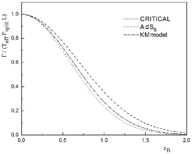
Figure 1: The decay widths of mesons vs. the position of flavor brane. The dash line belongs to the $AdS_{6}$ model, the dash-dot line belongs to the near-extremal KM model, and the dotted line is for the critical case.The decay width in the non-critical models are more than the critical one.

As mentioned before, the difference between equations (34) and (48) and the critical model [37] is the different effective string couplings. We use these equations and obtain the decay widths numerically. For this purpose, we put the values $R_{AdS}=\sqrt{\frac{15}{2}}$, $R^{\prime}_{AdS}=\sqrt{6}$ and $T_{\text{eff}}\approx 0.177~{}\text{GeV}^{2}$ into the equations (34),(48) and use equations (22),(45) to plot the decay width (fig. 1). From this diagram, we can see that the decay widths of mesons in the non-critical backgrounds of sections 2,3 are more than in the critical model. So we find larger values for the decay widths compared to the critical model.
Then we plot $\Gamma/M$ in terms of $M$ for two large-spin mesons, $a$ and $f$ by using a sigmoidal fitting for the experimental data of ref. [50] (see fig.2 ). From this diagram, we can see that the decay widths in the nature are not constant on the same Regge trajectory. The decay widths behave like equation (35) in which the effect of two massive endpoints of the string is considered.

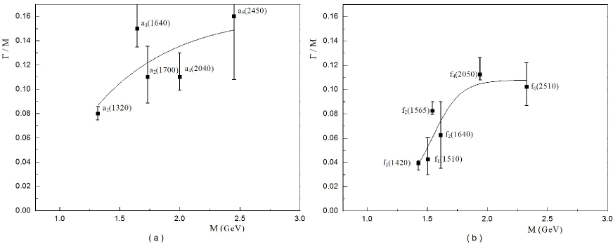
Figure 2: a) The decay width divided by mass versus the mass of the mesons states on the $a$ trajectory. b) The decay width divided by mass versus the mass of the mesons states on the $f$ trajectory. The solid lines correspond to a sigmoidal fitting for the data [50].

Also we can use equation (35) for the two non-critical models of sections 2,3 and the critical model [37] to plot $\Gamma/M$ in terms of $M$ (fig.3).
In this figure we can see that for the $a$ trajectory, there is a good agreement between the $AdS_{6}$ diagram and the experimental data for all spin values (the left diagram). For the $f$ trajectory we can see that our results deviate from the experimental results in low spins and the fitting of experimental data has a better agreement with the critical model of ref. [37] but for high spins in the $f$ trajectory, the $AdS_{5}\times S^{1}$ diagram is more compatible with the experimental data (the right diagram).

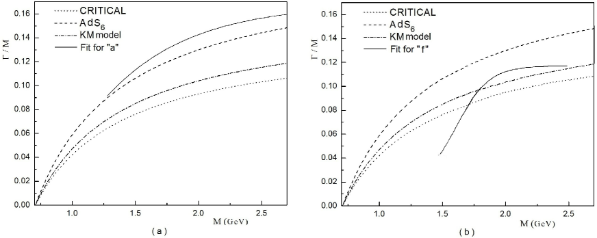
Figure 3: a) Comparison of the $\Gamma/M$ vs. $M$ for two non-critical models, critical model [37], and the fitting for $a$ meson. The dash line belongs to the $AdS_{6}$ model, the dash-dot line belongs to the $AdS_{5}\times S^{1}$ KM model, and the dotted line is for the critical case. The solid line is the fit for $a$ meson. b) Comparison of the $\Gamma/M$ vs. $M$ for two non-critical models, critical model [37], and the fitting for $f$ meson.

In this paper we used the non-critical string/gauge duality and obtained the decay widths for large-spin mesons. We chose two different six dimensional black hole backgrounds; the near extremal $AdS_{6}$ background and the near extremal KM model. By using the method of ref.[37], we obtained expressions for the decay widths and plotted it in terms of the position of the flavor brane (fig.1). From this diagram it is easy to see that the non-critical models lead to larger values for the decay width. Then we used another equation from ref. [39] and plotted the decay width in terms of the masses of meson states. We compared these results with the fitting of experimental data of ref. [50] for mesons $a$ and $f$ (fig.3). From these diagrams one can find that for $a$ meson, the $AdS_{6}$ background leads to a better result. Also for $f$ meson, the near extremal KM model has better agreement with data only for large spins. For lower spins, the critical model of ref. [37] is closer to the experimental data.

References

- [1] Maldacena J M 1998 The large N limit of superconformal field theories and supergravity Adv. Theor. Math. Phys. 2 231.
- [2] Witten E 1998 Anti-de Sitter space and holography Adv. Theor. Math. Phys. 2 253.
- [3] Schwarz J H 1999 Introduction to M Theory and AdS/CFT Duality (Lecture Notes in Physics vol 525) (Berlin: Springer) pp 1 21 (arXiv:hep-th/9812037).
- [4] Douglas M R and Randjbar-Daemi S 1999 Two lectures on AdS/CFT correspondence arXiv:hep-th/9902022.
- [5] Petersen J L 1999 Introduction to the Maldacena conjecture on AdS/CFT Int. J. Mod. Phys. A 14 3597.
- [6] Klebanov Igor R 2000 TASI lectures: introduction to the AdS/CFT correspondence arXiv:hep-th/0009139.
- [7] Herzog CP, Karch A, Kovtun P, Kozcaz C and Yaffe L G 2006 Energy loss of a heavy quark moving through N = 4 supersymmetric Yang Mills plasma J. High Energy Phys. JHEP07(2006)013 (arXiv:hep-th/0605158).
- [8] Herzog C P 2006 Energy loss of heavy quarks from asymptotically AdS geometries J. High Energy Phys. JHEP09(2006)032 (arXiv:hep-th/0605191).
- [9] Gubser S S 2006 Drag force in AdS/CFT Phys. Rev. D 74 126005.
- [10] Vazquez-Poritz J F 2008 Drag force at finite t Hooft coupling from AdS/CFT arXiv:hep-th/0803.2890.
- [11] Caceres E and Guijosa A Drag force in charged N = 4 SYM plasma J. High Energy Phys. JHEP11(2006)077.
- [12] Matsuo T, Tomino D andWenWY 2006 Drag force in SYM plasma with B field from AdS/CFT J. High Energy Phys. JHEP10(2006)055.
- [13] Sadeghi J, Setare M R, Pourhassan B 2009 Drag force with different charges in STU background and AdS/CFT J. Phys. G: Nucl. Part. Phys. 36 (2009) 115005 (19pp).
- [14] Sadeghi J, Setare M R, Pourhassan B and Hashmatian S 2009 Drag force of moving quark in STU background Eur. Phys. J. C 61 527 (arXiv:0901.0217 [hep-th]).
- [15] Sadeghi J and Pourhassan B 2008 Drag force of moving quark at the N = 2 supergravity J. High Energy Phys. JHEP12(2008)026 (arXiv:0809.2668 [hep-th]).
- [16] Nakano E, Teraguchi S and Wen W Y 2007 Drag force, jet quenching and AdS/QCD Phys. Rev. D 75 085016.
- [17] Liu H, Rajagopal K and Wiedemann U A 2006 Calculating the jet quenching parameter from AdS/CFT Phys. Rev. Lett. 97 182301.
- [18] Vazquez-Poritz J F 2006 Enhancing the jet quenching parameter from marginal deformations arXiv: hep-th/0605296.
- [19] Caceres E and GuijosaA2006 On drag forces and jet quenching in strongly coupled plasmas J. High Energy Phys. JHEP12(2006)068.
- [20] Lin F L and Matsuo T 2006 Jet quenching parameter in medium with chemical potential from AdS/CFT Phys. Lett. B 641 45.
- [21] Avramis S D and Sfetsos K 2007 Supergravity and the jet quenching parameter in the presence of R-charge densities J. High Energy Phys. JHEP01(2007)065.
- [22] Armesto N, Edelstein J D and Mas J 2006 Jet quenching at finite t Hooft coupling and chemical potential from AdS/CFT J. High Energy Phys. JHEP09(2006)039.
- [23] Edelstein J D and Salgado C A 2008 Jet quenching in heavy Ion collisions from AdS/CFT AIP Conf. Proc. 1031 207 (arXiv:0805.4515).
- [24] Fadafan K B 2008 Medium effect and finite t Hooft coupling correction on drag force and jet quenching parameter arXiv:0809.1336.
- [25] Peeters K, Sonnenschein J and Zamaklar M 2006 Holographic melting and related properties of mesons in a quark gluon plasma Phys. Rev. D 74 106008.
- [26] Liu H, Rajagopal K and Wiedemann U A 2007 An AdS/CFT calculation of screening in a hot wind Phys. Rev. Lett. 98 182301 (arXiv:hep-ph/0607062).
- [27] Chernicoff M, Garcia J A and Guijosa A 2006 The energy of a moving quark-antiquark pair in an N = 4 SYM plasma J. High Energy Phys. JHEP 09 068.
- [28] Erdmenger J, Evans N, Kirsch I and Threlfall E J 2008 Mesons in gauge/gravity duals Eur. Phys. J. A 35 81.
- [29] Sadeghi J and Heshmatian S 2010 Screening length of rotating heavy meson from AdS/CFT Int J Theor Phys 49 1811 (arXiv:hep-th/0812.4816).
- [30] Ali-Akbari M and B. Fadafan K 2009 Rotating mesons in the presence of higher derivative corrections from gauge-string duality arXiv:0908.3921v1 [hep-th].
- [31] Chernicoff M, Garcia J A and Guijosa A 2006 The energy of a moving quark-antiquark pair in an N = 4 SYM plasma J. High Energy Phys. JHEP09(2006)068.
- [32] Witten E 1998 Anti-de Sitter space, thermal phase transition, and confinement in gauge theories Adv. Theor. Math. Phys. 2 505 (arxiv:hep-th/9803131).
- [33] Sakai T and Sugimoto S 2004 Low Energy Hadron Physics in Holographic QCD (arXiv:hep-th/0412141v5); Sakai T and Sugimoto S 2005 More on a Holographic Dual of QCD (arXiv:hep-th/0507073v4) ; Hashimoto K Sakai T and Sugimoto S 2008 Holographic Baryons (arXiv:hep-th/0806.3122v3) ; Hata H Sakai T Sugimoto S and Yamato S 2007 Baryons from instantons in holographic QCD (arXiv:hep-th/0701280).
- [34] Kim K Y, Sin S J and Zahed I 2007 The Chiral Model of Sakai-Sugimoto at Finite Baryon Density arXiv:0708.1469v3 [hep-th]; Bergmann O, Lifschytz G and Lippert M 2007 Holographic Nuclear Physics JHEP 0711:056.
- [35] Kruczenski M, Zayas L A P, Sonnenschein J, and Vaman D (2005) Reggie trajectories for mesons in the holographic dual of large QCD JHEP 06 046 (arxiv:hep-th/0410035).
- [36] Rozali M et al. (2008) Cold nuclear matter in holographic QCD J. High Energy Phys. JHEP 0801 053; Sin S J, Yang S, Zhou Y (2009) Comments on Baryon Melting in Quark Gluon Plasma with gluon condensation (arXiv:hep-th/0907.1732v1); Curtis G et al. (1999) Baryons and string creation from the 5-brane world-volume action Nucl. Phys. B 547 127 1242;
- [37] Peeters K, Sonnenschein J and Zamaklar M (2006) Holographic decay of large-spin mesons (arxiv:hep-th/0511044v3).
- [38] Sjöstrand T (1982) The Lund Monte Carlo for jet fragmentation Comp. Phys. Commun 27 243; Andersson B (1998) The Lund model Cambridge University Press;Andersson B et al. (1983) Parton fragmentation and string dynamics Phys. Rep. 97 31.
- [39] Ida M (1978) Relativistic motion of massive quarkes joined by a massless string Prog. Theor. Phys. 59 1661.
- [40] Bigazzi F and Cotrone A L (2006) New predictions on meson decays from string splitting JHEP 0611:066 (arxiv:hep-th/0606059v2); Cotrone L A, Martucci L, and Troost W (2005) String splitting and strong coupling meson decay(arxiv:hep-th/0511045); Dai J and Polchinski J (1989) The decay of macroscopic fundamental strings Phys. Lett. B 220 387; Gupta K S and Rosenzweig C (1994) Semiclassical decat of excited string states on leading Regge Trajectories Phys. Rev. D 50 3368 (arxiv:hep-ph/9402263); Peeters K, Plefka J, and Zamakler M (2004) Splitting spinning strings in AdS/CFT JHEP 11 054 (arxiv:hep-th/0410275).
- [41] Wilkinson R B, Turok N, and Mitchell D (1990) The decay of highly excited closed strings Nucl. Phys. B 332 131.
- [42] Casher A, Neuberger H, and Nussinov S (1979) Chromoelectric flux tube model of particle production Phys. Rev. D 20 179-188.
- [43] Casero R, Paredes A, and Sonnenschein J (2005) Fundamental matter, meson spectroscopy and non-critical string/gauge duality (arxiv:hep-th/0510110).
- [44] Kuperstein S and Sonnenschein J (2004) Non-critical supergravity () and holography JHEP 0407 049 (arxiv:hep-th/0403254).
- [45] Bigazzi F et al. (2005) Non-critical holography and four-dimensional CFT’s with fundamentals JHEP 0510 012 (arxiv:hep-th/0505140).
- [46] Giveon A, Kutasov D, and Pelc O (1999) Holography for non-critical superstrings JHEP 10 035 (arxiv:hep-th/9907178).
- [47] Klebanov I R and Maldacena J M (2004) Superconformal gauge theories and non-critical superstrings Int. J. Mod. Phys. A 19 5003 (arxiv:hep-th/0409133).
- [48] Kuperstein S and Sonnenschein J (2004) Non-critical near extremal background as a holographic laboratory of four dimensional YM theory JHEP 0411 026.
- [49] Ferretti G, Kalkkinen J, and Martelli D (1999) Non-critical type 0 string theories and their field theory duals Nucl. Phys. B 555 135-156 (arxiv:hep-th/9904013); Armoni A, Fuchs E and Sonnenschein J (1999) Confinement in 4d yang-mills theories from non-critical type 0 string theory JHEP 06 027 (arxiv:hep-th/9903090); Ghoroku K, (2000) Yang-mills theory from non-critical string J. Phys. G 26 233-244 (arxiv:hep-th/9907143); Alvarez E, Gomez C, and Hernandez L (2001) Non-critical poincare invariant bosonic string backgrounds and closed string tachyons Nucl. Phys. B 600 185-196 (arxiv:hep-th/0011105); Murthy S (2003) Notes on non-critical superstrings in various dimensions JHEP 11 056 (arxiv:hep-th/0305197); Fotopoulos A, Niarchos V, and Prezas N (2005) D-branes and SQCD in non-critical superstring theory (arxiv:hep-th/0504010); Ashok S K, Murthy S, and Troost J (2005) D-branes in non-critical superstrings and minimal super Yang-Mills in various dimensions (arxiv:hep-th/0504079); Grassi P A and Oz Y (2005) Non-critical covariant superstrings (arxiv:hep-th/0507168).
- [50] Nakamura K et al. (Particle Data Group) (2010) J. Phys. G: Nucl. Part. Phys. 37 075021.