\begin{picture}(500.0,40.0)\par\put(0.0,58.0){\shortstack[l]{\small\it Gravitation \& Cosmology, \small\rm Vol. 12 (2006), No. 2-3 ({\bf{46-47}}), pp. 103--105 \\ \footnotesize{Proceedings of the International Conference on Gravitation, Cosmology, Astrophysics and Nonstationary Gas Dynamics,} \\ \footnotesize{Delicated to Prof. K.P.Staniukovich's 90th birthday, Moscow, 2-6 March 2006} \\ \footnotesize\copyright\ 2006 \ Russian Gravitational Society}} \par\end{picture}

EXACT STATIC SOLUTIONS FOR FLUID GRAVITATING BALLS

IN HOMOGENEOUS COORDINATES

A.M.Baranov and R.V.Bikmurzin
Dep. of Theoretical Physics,Krasnoyarsk State University, 79 Svobodny Av., Krasnoyarsk, 660041, Russia

Received 22 April 2006

Two new classes of exact interior static solutions of the Einstein equations in homogeneous coordinates for a gravitating ball filled by a Pascal perfect fluid are obtained. Schwarzschild’s interior solution of is a special case of these solutions.

1. Introduction

The choice of a coordinates’ system can simplify the representation of the Einstein equations. A spherically symmetric metric interval in 4D space-time is usually written in of the curvature coordinates. In this paper, we make use of the homogeneous coordinates according to the Weyl remark [1] that the 3D spherical metric interval is conformally flat in such coordinates. So the static spherically symmetric metric interval for an interior gravitational field of a fluid stellar model with a general distribution of mass density is written as

$$ds^{2}=A(r)dt^{2}-B(r)\left(dr^{2}+r^{2}(d\theta^{2}+\sin^{2}\theta\,d\varphi^{2})\right)=$$

$$=R_{0}^{2}(A(x)d{\tau{{}^{2}}}-B(x)dl^{2}).$$

Here we introduce the dimensionless coordinates $\tau=t/R_{0};\,x=r/R_{0};\,0\leq x\leq 1,$ where $t$ is the time variable; $r$ is the radial variable; $\theta;\varphi$ are angular variables; $R_{0}$ is a stellar exterior radius; $dl^{2}=(dx^{2}+x^{2}(d\theta^{2}+\sin^{2}\theta\,d\varphi^{2}));$ the velocity of light $c=1;\,$ $A(x)$ and $B(x)$ are metric functions.

2. The first class of solutions

The Einstein equations for the energy-momentum tensor of Pascal’s perfect fluid

$$T_{\alpha\beta}=\left(\mu(x)+p(x)\right)U_{\alpha}U_{\beta}-p(x)\,g_{\alpha\beta}$$

are transformed to three equations for $A(x)$ and $B(x)$ functions. The 4-velocity in a comoving frame of reference is equal to $U_{\alpha}=\delta^{0}_{\alpha}\sqrt{A(x)R_{0}^{2}}.$

In the case with $\mu=const\,$ (a homogeneous distribution of mass), one of these equations may be rewritten as Emden’s equation [2]

$$\frac{d^{2}b(x)}{dx^{2}}+\frac{2}{x}\frac{db(x)}{dx}+b(x)^{5}=0.$$

From this equation we can find the function $B(x)$ and then, from other gravitational equations, we obtain function $A(x)$ [3]

$$B_{Sch.}(x)=\frac{C_{1}}{(C_{2}+x^{2})^{2}},$$

$$A_{Sch.}(x)=\left[C_{4}-\frac{C_{3}}{(C_{2}+x^{2})}\right]^{2}.$$

Thus we have obtained Schwarzschild’s interior solution in homogeneous coordinates. The Weyl tensor is equal to zero for such exact solution which describes the conformally flat 4D space-time. The junction conditions on the stellar surface give connections of constants with compactness $\eta=2m/R_{0},$ where $m$ is Schwarzschild’s mass and $0\leq\eta<1$.

When $\mu(x)$ is a function of $x,$ we take the function $B(x)$ as a generalization of the case with a homogeneous distribution of mass density in the form

$$B_{in}(x)=\frac{C_{1}}{(C_{2}+x^{2})^{k}}=C_{1}Y(x)^{-k},$$

where $Y(x)=\left(C_{2}+x^{2}\right)$ and $0\leq k\leq 2$, then we can get functions $A_{in}(x)$, $\mu(x)$ and $\>p(x)$:

$$A_{in}(x)=\left[\frac{C_{4}Y(x)^{\Lambda}-C_{3}}{Y(x)^{(k+\Lambda-1)/2}}\right]^{2};$$

$$\mu(x)=\frac{kY(x)^{k-2}}{8\pi R^{2}_{0}C_{1}}\bigl{[}(2-k)Y(x)+(k+4)C_{2}\bigr{]};$$

$$p(x)=\frac{Y(x)^{k-2}}{4\pi R_{0}^{2}C_{1}}\biggl{[}Y(x)+7kC_{2}+\frac{C_{3}+C_{4}Y(x)^{\Lambda}}{C_{3}-C_{4}Y(x)^{\Lambda}}\times$$

$$\times\Lambda\bigl{(}(k-1)Y(x)-kC_{2}\bigr{)}\biggr{]}-3\mu(x),$$

where $\Lambda=\sqrt{2k^{2}-4k+1}\geq 0$ and the parameter $k$ can have values $k=\left(0;1-1/\sqrt{2}\right]\cup\left[1+1/\sqrt{2};2\right].$

In this case, the functions $B(x)$ and $\mu(x)$ are chosen as nonsingular functions for the stellar source. We also take the pressure equal to zero on the stellar surface.

So the metric interval (1) may be rewritten as

$$ds^{2}=\frac{R^{2}_{0}C_{1}}{Y(x)^{k}}\left[\frac{Y(x)^{1-\Lambda}}{C_{1}}(C_{4}Y(x)^{\Lambda}-C_{3})^{2}d\tau^{2}-dl^{2}\right]$$

Now we must find the constants $C_{1}$, $C_{2}$, $C_{3}$ and $C_{4}$ for a final result.

As an exterior solution, we take the Schwarzschild exterior solution in homogeneous dimensionless coordinates (see, e.g., [4])

$$A_{ext}(x)=\left(\frac{4x-\eta}{4x+\eta}\right)^{2},\quad B_{ext}(x)=\left(1+\frac{\eta}{4x}\right)^{4}.$$

Using the smooth junction conditions on the 2D stellar surface with the exterior solution in the form (10) in homogeneous coordinates, we have

$$C_{1}=\left(1+\frac{\eta}{4}\right)^{4}\left[\frac{k(4+\eta)}{2\eta}\right]^{k};$$

$$C_{2}=\frac{k(4+\eta)}{2\eta}-1;$$

$$C_{3}=\frac{k}{4\eta\Lambda}\Bigl{(}4k-(\eta-4)(k-1-\Lambda)\Bigr{)}\left[\frac{k(4+\eta)}{2\eta}\right]^{(k-3+\Lambda)/2};$$

$$C_{4}=\frac{k}{4\eta\Lambda}\Bigl{(}4k-(\eta-4)(k-1+\Lambda)\Bigr{)}\left[\frac{k(4+\eta)}{2\eta}\right]^{(k-3-\Lambda)/2}.$$

From a requirement $C_{2}>0$ it follows

$$\frac{k(\eta+4)}{2\eta}-1>0\;\;\Rightarrow\;\;k>\frac{2\eta}{\eta+4}\;\;\mbox{or}\;\;\eta<\frac{4k}{2-k}.$$

If the parameter $k$ is in the range $\left(0;1-1/\sqrt{2}\right]$, then the compactness $\eta$ has values in the interval $\left[0;\;4(\sqrt{2}-1)/(\sqrt{2}+1)\right)\approx\left[0;\;0.686\right).\,$ If $k>1+1/\sqrt{2},$ then parameter $\eta$ is arbitrary.

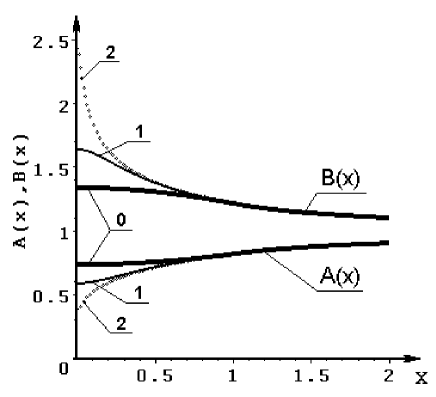
Figure 1: Behavior of the metric functions $A(x)=g_{00}(x)$ and $B(x)=g_{11}(x)$ of the complete solutions belonging to the first and second classes with $\eta=0.2$ and $k=0.1003$. The number 0 corresponds to Schwarzschild’s interior solution. The numbers 1 and 2 correspond to the first and second classes of solutions.

As a result, all functions of the first-class solutions may be rewritten in a clear form:

$$B_{in}(x)=\left(1+\frac{\eta}{4}\right)^{4}\left[1-\frac{2\eta}{k}\frac{(1-x^{2})}{\eta+4}\right]^{-k}=$$

$$=\left(1+\frac{\eta}{4}\right)^{4}\Psi(x)^{-k};$$

$$A_{in}(x)=\biggl{[}\frac{(\eta-4)(k-1-\Lambda)-4k}{2\Lambda(\eta+4)}\Psi(x)^{(1-k\Lambda)/2}\times$$

$$\times\bigl{(}1-\xi\Psi(x)^{\Lambda}\bigr{)}\Bigr{]}^{2};$$

$$\mu(x)=\frac{128\eta}{\pi R_{0}^{2}k}\frac{\Psi(x)^{k-2}}{(\eta+4)^{6}}\bigl{[}12k+\eta(k-2)(3-x^{2})\bigr{]},$$

where the following notations are used:

$$\xi=\frac{(\eta-4)(k-1+\Lambda)-4k}{(\eta-4)(k-1-\Lambda)-4k};$$

$$\Psi(x)=\biggl{[}1-\frac{2\eta}{k}\frac{(1-x^{2})}{(\eta+4)}\biggr{]}.$$

3. The second class of solutions

Now we shall generalize the function $A(x)$ from (4) by a similar way. The function $A(x)$ is defined as

$$A_{in}(x)=C_{1}(C_{2}-x^{2})=C_{1}Y(x)^{k}.$$

Then the Einstein equations give

$$B_{in}(x)=\left[\frac{Y(x)^{(\Lambda-1-k)/2}}{C_{4}Y(x)^{\Lambda}-C_{3}}\right]^{2};$$

$$p\>(x)=\frac{Y(x)^{k-\Lambda-1}}{8\pi R_{0}^{2}}\biggl{[}\Bigl{(}k^{2}\bigl{(}Y(x)-C_{2}\bigr{)}-2C_{2}(1+\Lambda)\Bigr{)}\times$$

$$\times\bigl{(}C_{3}+C_{4}Y(x)^{\Lambda}\bigr{)}^{2}+\Bigl{(}Y(x)(1+k^{2})+C_{2}(1+\Lambda-k^{2})\Bigr{)}\times$$

$$\times 4C_{3}C_{4}Y(x)^{\Lambda}+4C_{2}C_{3}^{2}\Lambda\biggr{]};$$

$$\mu(x)=\frac{k\bigl{(}C_{3}-C_{4}Y(x)^{\Lambda}\bigr{)}}{4\pi R_{0}^{2}Y(x)^{1+\Lambda-k}}\biggl{[}\Bigl{(}3C_{2}-\Lambda\bigl{(}Y(x)-C_{2}\bigr{)}\Bigr{)}\times$$

$$\times\bigl{(}C_{3}-C_{4}Y(x)^{\Lambda}\bigr{)}+2\Lambda C_{3}(Y(x)-C_{2})\biggr{]}-3p(x),$$

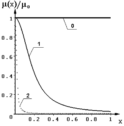
Figure 2: Behavior of the mass density $\mu(x)$ of the total solutions belonging to the first and the second classes with $\eta=0.2,$ $k=0.1003$ and a central mass density $\mu_{0}=const.$ The number 0 corresponds to Schwarzschils’s interior solution. The numbers 1 and 2 correspond to the first and the second classes of solutions.

where $\Lambda=\sqrt{1+2k^{2}}.$

Under the smooth junction conditions with Schwarzschil’s exterior solution, the new constants are

$$C_{1}=\left(\frac{4-\eta}{4+\eta}\right)^{2}\left[\frac{8\eta}{k(16-\eta^{2})}\right]^{k};$$

$$C_{2}=\frac{k(16-\eta^{2})}{8\eta}-1;$$

$$C_{3}=\frac{2\bigl{(}4(\Lambda+1)+k\eta)}{(\eta+4)^{2}\Lambda}\left[\frac{8\eta}{k(16-\eta^{2})}\right]^{(1+k-\Lambda)/2};$$

$$C_{4}=\frac{2(4(\Lambda-1)-k\eta)}{(\eta+4)^{2}\Lambda}\left[\frac{8\eta}{k(16-\eta^{2})}\right]^{(1+k+\Lambda)/2}.$$

Finally, we have bounds for the parameter $k$

$$\frac{80+40\eta-7\eta^{2}+\chi}{\eta^{3}-10\eta^{2}-64\eta+480}\geq\frac{k}{2}\geq\frac{4\eta}{(16-\eta^{2})},$$

where $\chi$ is

$$\chi=\sqrt{17\eta^{4}-240\eta^{3}+2528\eta^{2}-8960\eta+6400}.$$

4. Summary

The two classes of interior exact solutions of Einstein’s equations, found in the paper, describe the gravitational field of a ball filled with a Pascal perfect fluid. These solutions correspond to a static stellar model which is a generalization of Schwarzschild’s interior solution. Limiting conditions for the parameters have been found. The results of this study have been applied to a neutron star model with $\eta=0.2$ and the parameter $k=0.1003.$ Plots of the metric functions and the mass density have been constructed.

References

• [1] L.P.Eisenhart, “Riemannian Geometry”, Princeton
Univ. Press, Princeton, 1949.
• [2] G.Sansone, “Equazioni Differenziali Nel Campo Reale”, Bologna, Partre Seconda, 1949.
• [3] A.M.Baranov, R.V.Bikmurzin, Abstr. of Int. Seminar “Volga-16”, Kazan Univ., Kazan,2004, p.24-25.
• [4] N.M.Mitskievich, “Physical Fields in General Relativity”, Nauka, Moscow, 1969 (in Russian).