3D rotational diffusion microrheology using 2D video microscopy

R. Colin, M. Yan, L. Chevry, J.-F. Berret, B. Abou

Laboratoire Matière et Systèmes Complexes, UMR CNRS 7057, Université Paris Diderot
10, rue A. Domon et L. Duquet, 75205 Paris Cedex 13, France

We propose a simple way to measure the three-dimensional rotational diffusion of micrometric wires, using two-dimensional video microscopy. The out-of-plane Brownian motion of the wires in a viscous fluid is deduced from their projection on the focal plane of an optical microscope objective. An angular variable reflecting the out-of-plane motion, and satisfying a Langevin equation, is computed from the apparent wire length and its projected angular displacement. The rotational diffusion coefficient of wires between $1-100\,\mu$m is extracted, as well as the diameter distribution. Translational and rotational diffusion were found to be in good agreement. This is a promising way to characterize soft visco-elastic materials, and probe the dimension of anisotropic objects.

1 Introduction

Recording the three-dimensional (3D) motion of anisotropically shaped probes is a challenging issue. Although the theory of rotational Brownian motion has been established for a long time now ¹, the direct visualization and quantification of the Brownian motion of a micrometric anisotropic probe with a microscope is recent. It is due to the difficulty of quantifying the three-dimensional motion of the probe with two-dimensional (2D) optical techniques. It was first solved by studying the in-plane rotational motion of anisotropic probes ^{2, 3}. Recently, highly specialized optical techniques have opened new opportunities. Rotational diffusion was studied using light streak tracking of thin microdisks ^{4, 2}, depolarized dynamic light scattering and epifluorescence microscopy of optically anisotropic spherical colloidal probes ^{5, 6}, scanning confocal microscopy of colloidal rods with three-dimensional resolution ⁷, or reconstruction of the wire position from its hologram observed on the focal plane of a microscope ⁸. The rotation along the long axis was also investigated by analyzing the fluorescence images of rodlike tetramers ⁹. Following the 3D rotational diffusion of an optical probe thus remains costly in equipment, as well as in computational power.

From a practical point of view, micrometric probes can be used to determine the relation between stress and deformation in materials reducing significantly the sample volume, which may be crucial in biological samples ¹⁰. The technique, called microrheology, is a powerful tool to probe the rheological properties of complex fluids and biological materials at the micrometric scale. It can be achieved, either by recording the thermal fluctuations of probes immersed in the material, or by active manipulation of the probes ¹¹. While microrheology based on translational diffusion has been extensively investigated, the rotational diffusion of anisotropic objects remains poorly explored. However, it may be of great interest to investigate the length-scale dependent rheological properties of heterogeneous structured materials, such as complex fluids or biological tissues. In the case of anisotropic probes such as wires, the large aspect ratio of the probe allows for a detectable Brownian motion, over larger length scales, typically between $1-100\,\mu$m, than for spherical probes.

In this letter, we propose a simple way to measure the 3D rotational diffusion of micrometric wires, using 2D video microscopy. The 3D rotational Brownian motion of the wires immersed in a viscous fluid is extracted from their 2D projection on the focal plane of a microscope objective. An angular variable reflecting the out-of-plane motion of the wires and satisfying a Langevin equation, was computed from the apparent wire length and its projected angular displacement. The rotational diffusion coefficient was found to vary over more than $5$ decades, for wires of length between $1-100\,\mu$m and anisotropy ratios in the range $2-2000$. The resolution of the technique was quantified, by analyzing the wires trajectories. From these measurements, we were able to extract the distribution of the wires diameter, in good agreement with electron microscopy measurements. Rotational and translational diffusion measurements were compared, giving good agreement ^{12, 8}. This provides a new step towards the reliable use of rotational diffusion to characterize complex materials with an optical microscope, and probe the dimension of anisotropic objects.

2 Langevin equations for rotational diffusion

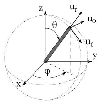
Figure 1: Spherical coordinate system $(r,\theta,\varphi)$ for a wire diffusing in a three-dimensional space. The unit vector ${\boldsymbol{\hat{u}_{r}}}$ is the wire orientational vector.

Let us consider a rigid wire diffusing in a stationary viscous fluid. Its rotational Brownian motion can be modeled by a Langevin equation, describing the fluctuations of the wire orientational unit vector ${\boldsymbol{\hat{u}_{r}}}$ (Fig. 1). In absence of an external torque, and neglecting inertia, the rotational equation of motion writes :

$$0=-{\zeta}_{R}\boldsymbol{\omega}+\boldsymbol{T_{r}}\,.$$ (1)

in which ${\zeta}_{R}\boldsymbol{\omega}$ and ${\boldsymbol{T_{r}}}$ are two effects from the fluid, respectively the viscous drag and the random Langevin torque. Since the wire is axisymmetric, the matrix of friction coefficients ${\zeta}_{R}$ is diagonal in the frame $({\boldsymbol{\hat{u}_{r}}},\boldsymbol{\hat{u}_{\theta}},\boldsymbol{\hat{u}_{\varphi}})$. The eigenvalue along ${\boldsymbol{\hat{u}_{r}}}$ describes the friction opposing the self-rotation of the wire around its main axis. The eigenvalues along $\boldsymbol{\hat{u}_{\theta}}$ and $\boldsymbol{\hat{u}_{\varphi}}$ are equal, and describe the friction opposing the rotation of the wire main axis.

The projection of the rotational Langevin equation (1) on the plane perpendicular to the wire $(\boldsymbol{\hat{u}_{\theta}},\boldsymbol{\hat{u}_{\varphi}})$, leads to :

$$-{\zeta_{R}}^{\bot}\boldsymbol{{\omega}^{\bot}}+\boldsymbol{T_{r}}^{\bot}=0\,,$$ (2)

where $\boldsymbol{{\omega}^{\bot}}$ and $\boldsymbol{T_{r}}^{\bot}$ are the components, respectively of the rotation vector and the Langevin random torque, in the plane $(\boldsymbol{\hat{u}_{\theta}},\boldsymbol{\hat{u}_{\varphi}})$, and ${\zeta_{R}}^{\bot}$ is the friction coefficient perpendicular to the wire axis. The projection of equation (1) along the wire axis will not be considered here ⁹.

The random torque $\boldsymbol{T_{r}}^{\bot}$ can be written as $\boldsymbol{T_{r}}^{\bot}=-T_{1}\left(t\right)\ \boldsymbol{\hat{u}_{\theta}}+T_{2}\left(t\right)\ \boldsymbol{\hat{u}_{\varphi}}$, where $T_{1}(t)$ and $T_{2}(t)$ are two Gaussian white-noise thermal driving torque, satisfying :

$$\langle T_{i}\left(t\right)\rangle_{i=1,2} = 0$$

$$\quad\langle T_{i}(t)T_{j}(t^{\prime})\rangle = 2{\zeta_{R}}^{\bot}k_{B}\mathrm{T}\delta_{i,j}\delta(t-t^{\prime})$$

with $\mathrm{T}$ the bath temperature, and $\langle\,\rangle$ refers to a time-averaged quantity.

For a finite cylinder – length $L$ and diameter $d$ – the perpendicular friction coefficient can be written in the form :

$${\zeta_{R}}^{\bot}=\frac{\pi\eta L^{3}}{3\,g\left(L/d\right)}$$ (3)

where $g\left(L/d\right)$ is a dimensionless function, which takes into account the finite-size effects of the wire. This function was analytically calculated for ellipsoids ¹³, and numerically approximated in the case of cylinders ^{1, 14, 15, 16, 17}.

The rotation vector $\boldsymbol{{\omega}^{\bot}}$ can be expressed as $\boldsymbol{{\omega}^{\bot}}=\dot{\theta}\,\boldsymbol{\hat{u}_{\varphi}}-\sin\theta\,\dot{\varphi}\,\boldsymbol{\hat{u}_{\theta}}$, and the projection of Eq. 2 in the plane $(\boldsymbol{\hat{u}_{\theta}},\boldsymbol{\hat{u}_{\varphi}})$ thus gives :

$${\zeta_{R}}^{\bot}\sin\theta\ \dot{\varphi}=T_{1}(t),\\ \qquad{\zeta_{R}}^{\bot}\dot{\theta}=T_{2}(t)$$

The angular variables $\psi(t)$, defined such as $\dot{\psi}=\sin\theta\ \dot{\varphi}$, and $\theta(t)$ both obey a one-dimensional Langevin equation, which respectively leads to :

$$\langle\Delta\psi^{2}(t)\rangle=2\frac{k_{B}\mathrm{T}}{{\zeta_{R}}^{\bot}}t =2D_{R}t$$ (4)

$$\quad\langle\Delta\theta^{2}(t)\rangle =2D_{R}t$$ (5)

where $D_{R}$ is the rotational diffusion coefficient. Computing Eqs. (4) and (3), the diffusion coefficient simply writes :

$$D_{R}=\frac{3k_{B}\mathrm{T}}{\pi\eta L^{3}}g(L/d)$$ (6)

In the general case of an out-of-plane rotational diffusion, Eqs. (4) and (5) show that determining the variables $\psi(t)$ or $\theta(t)$ will lead to the rotational diffusion coefficient $D_{R}$. From the 2D video recordings, both $\varphi(t)$ and $\sin\theta(t)$ were extracted. The variable $\Delta\psi(t)=\psi(t)-\psi(0)=\int_{0}^{t}dt^{\prime}\sin\theta(t^{\prime})\ \dot{\varphi}(t^{\prime})$ was then computed, leading to the determination of the mean-squared angular displacement $\langle\Delta\psi^{2}(t)\rangle$, and therefore to the rotational diffusion coefficient $D_{R}$.

3 Material and Methods

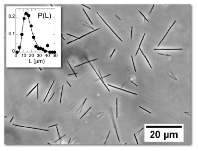
Figure 2: Optical microscopy images (X $40$) of a wire suspension. The distribution of the lengthes after synthesis can be fitted by a log-normal distribution, as shown in inset ($83$ wires). Due to a rather broad polydispersity, of the order of $0.5$ (defined as the standard deviation of $\ln{L}$), wires of length between $1$ to $100\,\mu$m were obtained. The distribution of the diameters was determined from electron microscopy, with a median diameter $0.4\,\mu$m, leading to anisotropy ratios between $2-2000$.

The wire formation results from the electrostatic co-assembly between oppositely charged iron oxide nanoparticles and polymers ¹⁷. The wires are purified and suspended in DI water. Figure 2 shows an optical microscopy image of the wire suspension after synthesis, and the corresponding length distribution in inset. In the present study, two batches of wires of length $15\,\mu$m (Fig. 2) and $30\,\mu$m are investigated ¹⁸. Due to a rather broad polydispersity in length, wires of length between $1$ and $100\,\mu$m were obtained. The distribution of the wires diameter was determined from electron microscopy, with a median diameter $0.4\,\mu$m, leading to anisotropy ratios between $2-2000$.

The aqueous wire suspension was then mixed with pure glycerol giving aqueous solutions of glycerol, also referred as wire suspensions. Aqueous solutions of glycerol with two different volume fractions, $50\%$ and $60\%$, were prepared. The wire suspension was then introduced in an observation chamber ($3\,\rm{mm}\times 3\,\rm{mm}\times 250\,\rm{\mu m}$) between a microscope slide and a coverslip, sealed with araldite glue to avoid evaporation and contamination of the sample.

An inverted Leica DM IRB microscope with a $\times 100$ oil immersion objective (NA=1.3, free working distance : $130\,\mu$m), coupled to a camera (EoSens Mikrotron) were used to record the 2D projection of the wires thermal fluctuations on the focal plane objective. The wires concentration was chosen diluted enough to prevent collisions and hydrodynamic coupling. They were always tracked far enough from the walls of the observation chamber. The microscope objective temperature was controlled within $0.1\,{{}^{\circ}}$ C, using a Bioptechs heating ring coupled to a home-made cooling device. The sample temperature was controlled through the oil immersion in contact. Sedimentation of the wires was negligible on the recording time scales.

The camera was typically recording $10$ images per second during $200$ s ($2000$ images). The 3D Brownian motion of the wires was extracted from their 2D projection on the $(x,y)$ plane (Fig. 1). The angle $\varphi(t)$ and the projected length $L(t)$ were measured from the images, using a home-made tracking algorithm, which is implemented as an ImageJ plugin¹⁹. Since the objective depth of focus ($1-2\,\mu$m) is shorter than the length of the wires, their out-of-plane image is distorted. The distorted image of a wire was seen as a cluster of connected pixels. The algorithm output is the length $L(t)$ of the cluster (projected length of the wire) and the angle $\varphi(t)$ of the cluster, as defined in figure 1. The algorithm mainly consists in three steps. First, a user-defined threshold is applied to the image. Then, the wire projection, seen as a set of connected pixels (cluster) is tracked at time $t$, in the vicinity of the position at time $t-1$. Finally, the cluster orientation and its length are computed, respectively giving the angle $\varphi(t)$, and the projected length $L(t)$. The position of the cluster center was also computed. Wires with a high out-of-plane angle, corresponding to angle $\theta$ smaller than $50$ degrees, could not be considered. Since the tracked wires are chosen to lie in the focal plane at the beginning of the recording, the length of the wire $L$ was taken as the maximum measured length $L(t)$ within the recording time, leading to $\sin\theta=L(t)/\max{(L(t))}$. The quantity $\Delta\psi(t)$ was computed by using the discrete equation $\Delta\psi(t,t_{0})=\sum_{t^{\prime}=t_{0}}^{t_{0}+t-\delta t}\frac{L(t^{\prime})}{L}\delta\varphi(t^{\prime})$, where $\delta\varphi(t^{\prime})=\varphi(t^{\prime}+\delta t)-\varphi(t^{\prime})$, and $\delta t$ is the time lapse between two images. A time average then enables us to compute $\langle\Delta\psi^{2}(t)\rangle=\langle\left(\Delta\psi^{2}(t,t_{0})\right)\rangle_{t_{0}}$.

The uncertainty on $\langle\Delta\psi^{2}(t)\rangle$ was evaluated including the uncertainties on $\varphi$, the projected length, and the total length. It also takes into account statistical accuracy. The uncertainty on the apparent length of an out-of-plane wire was determined by varying the $z$-position of the focal plane while recording the fixed wire. The corresponding computed lengths for different $z$-positions of the focal plane give an uncertainty of the apparent length as the wire moves along the axial direction. It was estimated to be $8\%$ for wires longer than $4\,\mu$m and $15\%$ below.

4 Rotational diffusion coefficient and diameters distribution

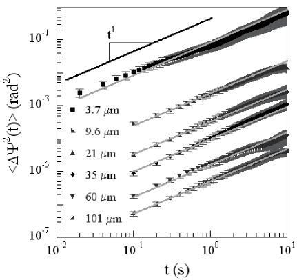
Figure 3: Mean-squared angular displacement (MSAD) of the wires as a function of the lag time, for wires of length between $3$ and $100\,\mu$m. The experiments were performed in an aqueous solution of glycerol ($50\%$ in volume). The MSAD increases linearly with time, as expected in a purely viscous fluid. The slope of each curve, corresponding to the diffusion coefficient, decreases with the length of the wire. Similar data were obtained in the $60\%$ in volume aqueous solutions of glycerol (not shown). The error bars include the uncertainties on $L$, $\varphi$ and statistical accuracy.

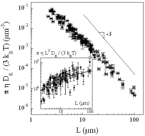
Figure 4: Rotational diffusion coefficient of the wires as a function of the wires length, normalised by viscosity and temperature. At first order, the diffusion coefficient scales as $L^{-3}$, as expected from Eq. (6). The dimensionless parameter $g_{rot}(L/d)=\frac{\pi\eta L^{3}}{3k_{B}\mathrm{T}}D_{R}$ is shown in inset as a function of the wires length. The gray line corresponds to the analytical expression established by Broersma, assuming a median diameter of $400$ nm. The large distribution of the data around the gray line reflects the distribution of the wires diameter.

The mean-squared angular displacement (MSAD) $\langle\Delta\psi^{2}(t)\rangle$ is shown in Fig. 3 as a function of the lag time $t$, for wires of length between $3\,\rm{\mu}$m and $100\,\rm{\mu}$m. The MSAD $\langle\Delta\psi^{2}(t)\rangle$ was found to increase linearly with time, as expected in a viscous fluid. From these curves, a rotational diffusion coefficient $D_{R}$ defined such as $\langle\Delta\psi^{2}(t)\rangle=2D_{R}t$, could then be extracted. Figure 4 shows the rescaled quantity $\frac{\pi\eta}{3k_{B}\mathrm{T}}D_{R}$ as a function of the measured length of the wire $L$. At leading order, the diffusion coefficient decreases as $L^{-3}$, over $5$ decades. A correction $g_{rot}(L/d)$ for the finite-size effects of the wire is expected, as described in Eq. (6). The rescaled diffusion coefficient $\frac{\pi\eta}{3k_{B}\mathrm{T}}D_{R}$ was then multiplied by $L^{3}$, leading to the experimental determination of the dimensionless function $g_{rot}(L/d)$ (Fig. 4-inset).

The resolution of the technique was quantified from the wires trajectories using the relation :

$$\langle\Delta\psi^{2}(t)\rangle=2D_{R}(t-\sigma/3)+2\epsilon_{rot}^{2}$$ (7)

including the measurement error $\epsilon_{rot}$, and corrected for the camera exposure time $\sigma$ ^{12, 8}. The measurement error $\epsilon_{rot}$ was found to decrease with the length of the wire, as shown in figure 5. It typically corresponds to an error in orientation of $4^{\circ}$ for a $10\,\mu$m long wire. The largest error was obtained for short wires, of $2$ to $3$ micrometers long, where an error of orientation of roughly $8^{\circ}$ was found. For the longest wires above $20\,\mu$m, the error was found to be less than $1^{\circ}$.

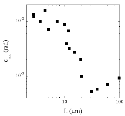
Figure 5: Measurement error $\epsilon_{rot}$ as a function of the length of the wires. The error in orientation is around $4^{\circ}$ for a $10\,\mu$m long wire. The largest error was obtained for short wires, of $2$ to $3$ micrometers long, where an error of orientation of roughly $8^{\circ}$ was found. For the longest wires above $20\,\mu$m, the error was found to be less than $1^{\circ}$.

An analytical expression for the finite-size effects function $g_{rot}(L/d)$ was established by Broersma in 1960 ^{20, 16}. It is expected to be valid for $p=L/d>4.6$, and writes :

$$g_{rot}(p)=\ln\left(p\right)-0.446-\frac{0.2}{\ln\left(2p\right)}$$

$$-\frac{16}{\ln\left(2p\right)^{2}}+\frac{63}{\ln\left(2p\right)^{3}}-\frac{64}{\ln\left(2p\right)^{4}}$$ (8)

Fig. 4-inset shows the Broesma relation (8), using a median diameter $d=400$ nm. The large distribution of the data around this adjustment reflects the distribution of the diameter of the wires.

By numerically inverting the relation (8), we could extract the distribution of the wires diameter. The corresponding values of $p=L/d$ range between $2$ and $2000$. A small fraction of the wires (less than $5\%$) exhibit a value of $p$ which is smaller than the validity range established by Broersma ($p>4.6$). More recently, another analytical expression, valid for $2<p<20$, was proposed by Tirado et al. ¹⁴. This expression was used for the few wires falling out of the validity range of Broersma’s theory, and for which Tirado’s expression is valid.

Figure 6 shows the distribution of the diameters obtained from the diffusion measurements, also compared to the one obtained from Scanning Electron Microscopy (SEM) measurements. The distributions have been fitted by log-normal distributions, leading to equal median diameters $0.4\,\rm{\mu}$m. The polydispersities (standard deviations of $\ln d$) are respectively ${\sigma_{d}}_{\rm micro}=0.53$ and ${\sigma_{d}}_{\rm SEM}=0.38$. The distributions are in good agreement, the largest discrepencies come for the smallest diameters, where the precision of our method is the lowest, because of the high non-linearity of the function $g_{rot}(L/d)$ as a function of $d$.

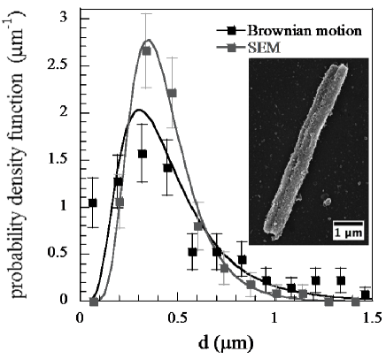
Figure 6: Distribution of the wires diameter, extracted from the wires Brownian motion measurements. The distributions are fitted by log-normal distributions, leading to equal median diameters $0.4\,\rm{\mu}$m. The polydispersities are respectively ${\sigma_{d}}_{\rm micro}=0.53$ and ${\sigma_{d}}_{\rm SEM}=0.38$. The distributions, obtained with differents methods are in good agreement. In inset, scanning electron microscopy of a wire.

We now compare rotational and translational fluctuations. The translational fluctuations of the wires were measured in the wire’s frame of reference. In our experiments, only the component of the center-of-mass translation along $\boldsymbol{\hat{u}_{\varphi}}$ could be measured. Since the diffusion in the $z$-direction could not be evaluated, the translational diffusion parallel to the wire, along ${\boldsymbol{\hat{u}_{r}}}$, and the one along $\boldsymbol{\hat{u}_{\theta}}$ were not accessible. Figure 7 shows the center-of-mass mean-squared displacement $\langle\Delta r_{\varphi}^{2}(t)\rangle=\langle((\boldsymbol{r}(t+t^{\prime})-\boldsymbol{r}(t^{\prime}))\cdot\boldsymbol{\hat{u}_{\varphi}}(t^{\prime}))^{2}\rangle_{t^{\prime}}$ for wires, between $3$ and $100\,\mu$m. It was found to increase linearly with the lag time, as expected in a viscous fluid. The data of translational diffusion were fitted according to the relation ¹²:

$$\langle\Delta r_{\varphi}^{2}(t)\rangle=2D_{transl}^{\perp}(t-\sigma/3)+2\epsilon_{transl}^{2}$$ (9)

including the measurement error $\epsilon_{transl}$ and corrected for the camera’s exposure time $\sigma$. The translational diffusion coefficient writes :

$$D_{transl}^{\perp}=\frac{k_{B}T}{4\pi\eta L}g_{transl}^{\perp}(p)$$ (10)

with the finite-size effect function $g_{transl}^{\perp}(p)=ln(p)+0.839+0.185/p+0.233/p^{2}$¹⁴. The measurement error $\epsilon_{transl}$ is shown in Figure 7 (inset) for wires of length between $3$ and $100\,\mu$m. It was found to be less than $\epsilon_{transl}=0.3$ pixel in most cases, which means that the center of the wire was tracked with a precision better than $40$ nm in the $(x,y)$ plane.

Fitting Eqs (7) and (9) for a given wire gives the values $D_{R}$ and $D_{transl}^{\perp}$ of the diffusion coefficients, respectively obtained with rotational and translational measurements. Given the experimental conditions, this respectively yields values of $\ln(p)$, $\ln(p_{rot})$ and $\ln(p_{transl})$, according to Eqs. (6) and (10). Table 1 presents a comparison between rotational and translational measurements for wires of length between $4$ and $95\,\mu$m. The values of $\ln(p)$ obtained with rotational and translational measurements were found to be in good agreement.

$L(\mu\rm{m})$	$D_{R}\,(\rm{rad}^{2}/$s)	$10^{3}D_{transl}^{\perp}\,(\mu\rm{m}^{2}/$s)	$\ln(p_{rot})$	$\ln(p_{transl})$
$4.4$	$0.016\pm 0.004$	$39\pm 4$	$3.3\pm 1.1$	$3.4\pm 0.6$
$9.8$	$(1.3\pm 0.2)10^{-3}$	$17.9\pm 0.7$	$3.2\pm 0.7$	$3.6\pm 0.3$
$35$	$(4.9\pm 0.2)10^{-5}$	$6.7\pm 0.2$	$5.2\pm 0.7$	$5.2\pm 0.2$
$95$	$(2.8\pm 0.1)10^{-6}$	$3.1\pm 0.2$	$5.8\pm 0.7$	$6.8\pm 0.5$

Table 1: Comparison between rotational and translational measurements for wires of various lengths. The values of $\ln(p)$ obtained with rotational and translational measurements, respectively $\ln(p_{rot})$ and $\ln(p_{transl})$, are in good agreement.

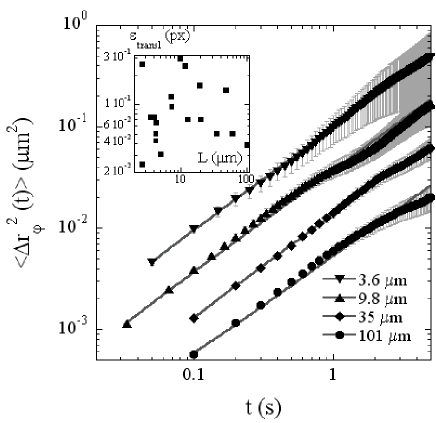
Figure 7: Mean-squared displacement of the center-of-mass of the wires of length between $3$ and $100\,\mu$m. The MSD increases linearly with time, as expected in a purely viscous fluid. The lines correspond to the fits according to Eq. (9). Inset: measurement error $\epsilon_{transl}$ for wires of various lengths.

5 Conclusion

In this letter, we propose a simple way to follow the 3D rotational Brownian motion of micrometric wires in a viscous fluid, from the 2D projection of the wires on the focal plane of a microscope. The rotational diffusion coefficient of the wires between $1-100~{}\mu$m was computed as a function of the wires length, ranging over $5$ decades. The resolution of the technique was quantified, by analyzing the wires trajectories. Our diffusion measurements allow us to extract the distribution of the wires diameter, in good agreement with SEM measurements. Rotational and translational diffusion measurements were compared and found to be in good agreement ^{12, 8}. This technique provides a simple way to measure the out-of-plane rotational diffusion of a wire in a viscous fluid, opening new opportunities in microrheology to characterize more complex fluids, and probe the dimension of anisotropic objects.

6 Acknowledgements

We thank O. Sandre and J. Fresnais from the Laboratoire Physico-chimie des Electrolytes, Colloïdes et Sciences Analytiques (UMR CNRS 7612) for providing us with the magnetic nanoparticles. This research was supported by the ANR (ANR-09-NANO-P200-36) and the European Community through the project NANO3T (number 214137 (FP7-NMP-2007-SMALL-1).

References

- 1 Masao Doi and S. F. Edwards. Theory of polymer dynamics. Oxford University Press, 1986.
- 2 C. Wilhelm, J. Browaeys, A. Ponton, and J.-C. Bacri. Rotational magnetic particles microrheology: The maxwellian case. Phys. Rev. E, 67(1):011504, 2003.
- 3 Y. Han, A. M. Alsayed, M. Nobili, J. Zhang, T. C. Lubensky, and A. G. Yodh. Brownian Motion of an Ellipsoid. Science, 314(5799):626–630, 2006.
- 4 Z. Cheng and T. G. Mason. Rotational diffusion microrheology. Phys. Rev. Lett., 90(1):018304, 2003.
- 5 Efrén Andablo-Reyes, Pedro Díaz-Leyva, and José Luis Arauz-Lara. Microrheology from rotational diffusion of colloidal particles. Phys. Rev. Lett., 94:106001, 2005.
- 6 Stephen M. Anthony, Liang Hong, Minsu Kim, and Steve Granick. Single-particle colloid tracking in four dimensions. Langmuir, 22(24):9812–9815, 2006.
- 7 Deshpremy Mukhija and Michael J. Solomon. Translational and rotational dynamics of colloidal rods by direct visualization with confocal microscopy. J. Chem. Phys., 314(1):98 – 106, 2007.
- 8 Fook C. Cheong and David G. Grier. Rotational and translational diffusion of copper oxide nanorods measured with holographic video microscopy. Opt. Express, 18(7):6555–6562, 2010.
- 9 Liang Hong, Stephen M. Anthony, and Steve Granick. Rotation in suspension of a rod-shaped colloid. Langmuir, 22(17):7128–7131, 2006.
- 10 B. Abou, C. Gay, B. Laurent, O. Cardoso, D. Voigt, H. Peisker, and S. Gorb. Extensive collection of femtoliter pad secretion droplets in beetle leptinotarsa decemlineata allows nanoliter microrheology. J. R. Soc. Interface, 7:1745–1752, 2010.
- 11 T. A. Waigh. Microrheology of complex fluids. Rep. Prog. Phys., 68:685–742, 2005.
- 12 T. Savin and P. Doyle. Static and dynamic errors in particle tracking microrheology. Biophysical Journal, 88:623 –638, 2005.
- 13 Francis Perrin. Mouvement brownien d’un ellipsoide (i). dispersion diélectrique pour des molécules ellipsoidales. Journal de Physique et Le Radium, 5(10):497–511, Octobre 1934.
- 14 Mercedes Tirado, Carmen López Martinez, and José García de la Torre. Comparison of theories for the translational and rotational diffusion coefficients of rod-like macromolecules. application to short dna fragments. J. Chem. Phys., 81(4):2047–2052, 1984.
- 15 S. Broersma. Viscous force constant for a closed cylinder. J. Chem. Phys., 32:1632–1635, 1960.
- 16 S. Broersma. Viscous force and torque constants for a cylinder. J. Chem. Phys., 74(12):6989–6990, 1981.
- 17 J. Fresnais, J.-F. Berret, B. Frka-Petesic, Olivier Sandre, and R. Perzynski. Electrostatic co-assembly of iron oxide nanoparticles and polymers: Towards the generation of highly persistent superparamagnetic nanorods. Advanced Materials, 20(20):3877–3881, 2008.
- 18 M. Yan, J. Fresnais, and J.-F. Berret. Growth mechanism of nanostructured superparamagnetic rods obtained by electrostatic co-assembly. Soft Matter, 10:1997–2005, 2010.
- 19 W. S. Rasband. ImageJ, U. S. National Institutes of Health, Bethesda, Maryland, USA, http://imagej.nih.gov/ij/. 1997-2011.
- 20 S. Broersma. Rotational diffusion constant of a cylindrical particle. J. Chem. Phys., 32(6):1626–1631, 1960.