Slow-roll freezing quintessence

Abstract

We examine the evolution of quintessence models with potentials satisfying $(V^{\prime}/V)^{2}\ll 1$ and $V^{\prime\prime}/V\ll 1$, in the case where the initial field velocity is nonzero. We derive an analytic approximation for the evolution of the equation of state parameter, $w$, for the quintessence field. We show that such models are characterized by an initial rapid freezing phase, in which the equation of state parameter $w$ decreases with time, followed by slow thawing evolution, for which $w$ increases with time. These models resemble constant-$V$ models at early times but diverge at late times. Our analytic approximation gives results in excellent agreement with exact numerical evolution.

I Introduction

Cosmological data from a wide range of sources including type Ia supernovae union08 ; perivol ; hicken , the cosmic microwave background Komatsu , baryon acoustic oscillations bao ; percival , cluster gas fractions Samushia2007 ; Ettori and gamma ray bursts Wang ; Samushia2009 seem to indicate that at least 70% of the energy density in the universe is in the form of an exotic, negative-pressure component, called dark energy.

The dark energy component is usefully parameterized by its equation of state parameter, defined as the ratio of its pressure to its density:

$$w=p_{\rm DE}/\rho_{\rm DE}.$$ (1)

Observations constrain $w$ to be very close to $-1$. For example, if $w$ is assumed to be constant, then $-1.1\ {\raise-2.15277pt\hbox{$\buildrel<\over{\sim}$}}\ w\ {\raise-2.15277pt\hbox{$\buildrel<\over{\sim}$}}\ -0.9$ Wood-Vasey ; Davis .

While a cosmological constant ($w=-1$) remains consistent with the observations, a variety of other models have been proposed in which $w$ is time varying. A common approach is to use a scalar field $\phi$ as the dark energy component. The class of models in which the scalar field is canonical is dubbed quintessence RatraPeebles ; CaldwellDaveSteinhardt ; LiddleScherrer ; SteinhardtWangZlatev and has been extensively studied. (See Ref. Copeland for a recent review).

A related, yet somewhat different approach is phantom dark energy, i.e., a component for which $w<-1$, as first proposed by Caldwell Caldwell . Such models have well-known problems CarrollHoffmanTrodden ; ClineJeonMoore ; BuniyHsu ; BuniyHsuMurray (however see Creminelli:2008wc ; Cai for recent attempts to construct a stable model), but nevertheless have been widely studied as potential dark energy candidates.

These models allow considerable freedom in the choice of the potential $V(\phi)$, leading to an infinite set of possible models and corresponding behaviors for the evolution $w$ as a function of the redshift $z$. It would therefore be a considerable simplification if one could find an interesting subset of such models that converged to a single trajectory or a well-defined set of trajectories for $w(z)$. One approach that yields such a simplification was considered by Scherrer and Sen ScherrerSen1 , who examined the evolution of a scalar field in a “nearly flat” potential, where the flatness condition consisted of the slow-roll conditions familiar from inflation:

$$\lambda^{2}\equiv\left(-\frac{1}{V}\frac{dV}{d\phi}\right)^{2}\ll 1,$$ (2)

$$\left|\frac{1}{V}\frac{d^{2}V}{d\phi^{2}}\right|\ll 1.$$ (3)

As in Ref. ScherrerSen1 , we will assume for definiteness that $dV/d\phi<0$ and $\lambda>0$, but of course none our results will depend on this choice. Note that while equations (2) and (3) are the familiar slow-roll conditions from inflation, the evolution of the scalar field is very different for the case of quintessence, since in that case one must also include the effect of the matter density on the expansion rate.

Ref. ScherrerSen1 considered models satisfying equations (2) and (3) in which the field is initially at rest, so that $w\approx-1$ at early times, and $w$ increases at late times as the field rolls down the potential; in the terminology of Ref. CL , these are “thawing” models. Then equation (2) ensures that $w$ remains close to $-1$, while equations (2) and (3) taken together indicate that $\lambda$ is nearly constant. For all potentials satisfying these conditions, it can be shown that the behavior of $w$ can be accurately described by a unique function of $\Omega_{\phi}$ (the fraction of the total density contributed by the quintessence field, where we assume a flat universe) and the (assumed constant) value of $\lambda$ ScherrerSen1 . In ScherrerSen2 this result was extended to phantom models satisfying Eqs. (2-3).

In this paper, we relax the initial condition that $\dot{\phi}\equiv d\phi/dt=0$, so that $w\neq-1$ initially, but we retain both slow roll conditions on the potential (equations 2 and 3). This allows us to extend the formalism of Ref. ScherrerSen1 to models in which $w$ decreases toward $-1$ at late times, rather than increasing away from $-1$; the former models are called “freezing” models CL .

Note that the slow roll conditions, Eqs. (2-3), while sufficient to ensure $w\approx-1$ today, are not necessary, and many other attempts to classify or simplify the set of quintessence trajectories have been proposed. For example, if equation (2) holds, but equation (3) is relaxed, one still has $w\approx-1$, but there is now an extra degree of freedom, the value of $V^{\prime\prime}/V$. Instead of a single solution for the evolution of $w$, one obtains a well-defined family of solutions ds1 . (This family of solutions includes the slow-roll solution of Ref. ScherrerSen1 as a special case in the limit where $V^{\prime\prime}/V\rightarrow 0$). These models were explored in more detail in Refs. ds2 ; ds3 ; chiba .

Other attempts to systematize the behavior of dark-energy quintessence fields based on other assumptions have been given in Refs. Watson ; Crit ; Neupane ; Cahn ; Chiba ; Cortes ; Bond ; Luo . Where these other approaches overlap those of this paper, further discussion and comparison with our results will be given below.

In the next section, we examine the evolution of $w$ for slow-roll potentials with the assumption that $\dot{\phi}\neq 0$ initially. In Sec. III, we compare our predictions for $w(a)$ with exact numerical results. Our conclusions are discussed in Sec. IV.

II Evolution of $w$: Analytic results

We will assume that the dark energy is provided by a minimally-coupled scalar field, $\phi$, with equation of motion given by

$$\ddot{\phi}+3H\dot{\phi}+\frac{dV}{d\phi}=0,$$ (4)

where $H$ is the Hubble parameter, given by

$$H=\left(\frac{\dot{a}}{a}\right)=\sqrt{\rho/3}.$$ (5)

Here $a$ is the scale factor, $\rho$ is the total density, and we take $8\pi G=1$ throughout. Equation (4) indicates that the field rolls downhill in the potential $V(\phi)$, but its motion is damped by a term proportional to $H$.

The pressure and density of the scalar field are given by

$$p=\frac{\dot{\phi}^{2}}{2}-V(\phi),$$ (6)

and

$$\rho=\frac{\dot{\phi}^{2}}{2}+V(\phi),$$ (7)

respectively, and the equation of state parameter, $w$, for the quintessence field is given by equation (1).

As in Ref. ScherrerSen1 , we note that the equations simplify if we express $w$ as a function of $\Omega_{\phi}$, giving

$$\frac{dw}{d\Omega_{\phi}}=\frac{-3(1+w)(1-w)+\lambda(1-w)\sqrt{3(1+w)\Omega_{\phi}}}{3(-w)\Omega_{\phi}(1-\Omega_{\phi})}.$$ (8)

(See Ref. ScherrerSen1 for the details of this derivation).

Consider a scalar field moving in a potential that satisfies equations (2) and (3), and assume we are in a regime such that $1+w\ll 1$. Note that in relaxing the initial condition that $\dot{\phi}=0$, it is possible to have transient evolution with $w$ far from $-1$ even when equations (2) and (3) are satisfied. Here we assume that the evolution has proceeded far enough that $1+w\ll 1$, but $w\neq-1$, when we begin to examine the evolution. With these assumptions, equation (8) simplifies to ScherrerSen1

$$\frac{dw}{d\Omega_{\phi}}=-\frac{2(1+w)}{\Omega_{\phi}(1-\Omega_{\phi})}+\frac{2}{3}\lambda_{0}\frac{\sqrt{3(1+w)}}{(1-\Omega_{\phi})\sqrt{\Omega_{\phi}}},$$ (9)

where $\lambda_{0}$ is the (assumed constant) value of $\lambda$. The general solution of equation (9) is

$$1+w=\frac{1}{3}\lambda_{0}^{2}$$

$$\times\left[\frac{1}{\sqrt{\Omega_{\phi}}}-\left(\frac{1}{\Omega_{\phi}}-1\right)\left(\tanh^{-1}\left(\sqrt{\Omega_{\phi}}\right)+C\right)\right]^{2}.$$ (10)

The constant $C$ parametrizes different initial values of $\dot{\phi}$, and therefore characterizes different evolutionary trajectories. Ref. ScherrerSen1 considered only the case $C=0$, which corresponds to $\dot{\phi}=0$ initially, giving

$$1+w=\frac{1}{3}\lambda_{0}^{2}$$

$$\times\left[\frac{1}{\sqrt{\Omega_{\phi}}}-\left(\frac{1}{\Omega_{\phi}}-1\right)\tanh^{-1}\sqrt{\Omega_{\phi}}\right]^{2}.$$ (11)

Equation (II), derived as one of the main results in Ref. ScherrerSen1 , displays a purely thawing behavior, as the field begins initially with $w=-1$, and $w$ increases as $\phi$ rolls down the potential. Note that at early times, when $\Omega_{\phi}\ll 1$, we can expand equation (II) to give

$$1+w=\frac{1}{3}\lambda_{0}^{2}\left[\frac{2}{3}\Omega^{1/2}+\frac{2}{15}\Omega^{3/2}+\frac{2}{35}\Omega^{5/2}+...\right]^{2}.$$ (12)

Retaining only the first term in this expansion gives

$$1+w=\frac{4}{27}\lambda_{0}^{2}\Omega_{\phi}.$$ (13)

This agrees with the result of Cahn, de Putter, and Linder Cahn , who defined a “flow parameter” $F\equiv(1+w)/\lambda_{0}^{2}\Omega_{\phi}$ and showed that $F=4/27$ in the limit considered here.

Equation (II) when $C\neq 0$ corresponds to the case where the field has $\dot{\phi}\neq 0$ initially. The case $C<0$ corresponds to a field rolling down the potential, while $C>0$ gives solutions for the field rolling uphill initially. While the latter possibility might seem somewhat contrived, it has been considered previously Csaki ; Sahlen1 ; Sahlen2 and we include it here for completeness.

The actual value of $C$ depends in the initial value of $\dot{\phi}$, but it is easiest to evaluate $C$ in terms of the value of $w$ corresponding to some initial value of $\Omega_{\phi}$. If we designate these values as $w_{i}$ and $\Omega_{\phi i}$, respectively, and take an early enough epoch that $\Omega_{\phi i}\ll 1$, then we have

$$C=\pm\frac{\sqrt{3(1+w_{i})}\Omega_{\phi i}}{\lambda_{0}},$$ (14)

where the sign of $C$ is determined by whether the field is rolling initially up or down the potential. In terms of $\dot{\phi}$, we simply have $1+w_{i}\approx\dot{\phi}^{2}/V_{i}$, where $V_{i}$ is the (initial but assumed nearly constant) value of the potential.

In equation (II) $w$ enters only in the combination $(1+w)/\lambda_{0}^{2}$. In the left panel of Fig. 1, we display this quantity as a function of $\Omega_{\phi}$ for the indicated values of $C\leq 0$. Except for $C=0$, the generic behavior of these models is an initial freezing period, during which $w$ decreases rapidly with time, followed by a period of thawing, with a much slower increase of $w$ with time.

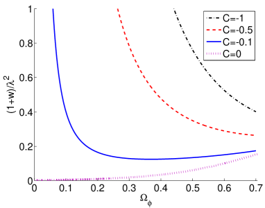
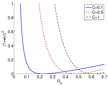
Figure 1: The value of $(1+w)/\lambda_{0}^{2}$ as a function of $\Omega_{\phi}$ for the indicated values of C. Here $w$ is the equation of state parameter for the quintessence field, $\Omega_{\phi}$ is the fraction of the total density contributed by the quintessence field, and $\lambda_{0}$ is the value of $-(1/V)(dV/d\phi)$ (taken to be constant).

The value of $\Omega_{\phi}$ for which $1+w$ reaches a minimum, corresponding to the transition between freezing and thawing behavior, can easily be derived from equation (II):

$$C=\sqrt{\Omega_{\phi}}-\tanh^{-1}\sqrt{\Omega_{\phi}}.$$ (15)

Thus, models with $-C\ {\raise-2.15277pt\hbox{$\buildrel>\over{\sim}$}}\ 0.5$ are still freezing at the present. On the other hand, it is clear from Fig. 1 that models with $-C\ {\raise-2.15277pt\hbox{$\buildrel<\over{\sim}$}}\ 0.1$ are nearly indistinguishable from the $C=0$ case, as they enter the thawing period when $\Omega_{\phi}\ll 1$.

In the right panel of Fig. 1, we show the corresponding evolution of $(1+w)/\lambda_{0}^{2}$ as a function of $\Omega_{\phi}$ for $C>0$. These models show more complex behavior, as the field first rolls uphill, stops (giving $w=-1$), and then rolls back down again. The value of $\Omega_{\phi}$ at which $w=-1$ is given by

$$C=\frac{\sqrt{\Omega_{\phi}}}{\left(1-\Omega\right)}-\tanh^{-1}\sqrt{\Omega_{\phi}}.$$ (16)

Since we always assume $1+w\ll 1$, we can express $w$ as a function of the scale factor $a$ by taking $\Omega_{\phi}$ to be well-approximated by its value for a $\Lambda$CDM universe ScherrerSen1 :

$$\Omega_{\phi}=\left[1+\left(\Omega_{\phi 0}^{-1}-1\right)a^{-3}\right]^{-1}.$$ (17)

Equations (II) and (17) together then provide an analytic approximation for $w(a)$ for these models. In Fig. 2, we show $(1+w)/\lambda_{0}^{2}$ as a function of the scale factor for the same set of models as in Fig. 1, where we have taken $\Omega_{\phi 0}=0.7$ and $a=1$ at the present.

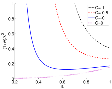
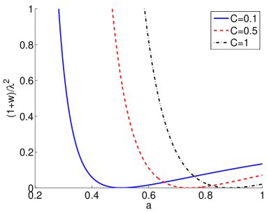
Figure 2: As Fig. 1, with the scale factor $a$ (taken to be 1 at the present) on the horizontal axis, and $\Omega_{\phi 0}=0.7$.

III Comparison with exact evolution

We now test the accuracy of the analytic approximation derived in the previous section by comparing our analytic predictions for $w(a)$ with an exact numerical integration of the equations of motion. Although we expect our approximation to apply to any potential with a region in $\phi$ satisfying equations (2) and (3), we will consider here two representive examples:

• Linear potential

  $$V\left(\phi\right)=V_{0}-\alpha\phi$$ (18)

  where take $\alpha=0.1$.

• Power-Law potential

  $$V\left(\phi\right)=V_{0}\phi^{-n}$$ (19)

  where we take $n=0.1.$

In both of these cases the parameters of the potential were chosen so as to satisfy the slow-roll conditions (equations 2 and 3), so that $\lambda$ is roughly constant and $\ll 1$. We set the initial value of $w$ to $w_{i}=-0.95$ and $\lambda_{0}=-0.08$. Then the initial value of $\Omega_{\phi}$ is chosen to give $C=\pm 0.1$, $C=\pm 0.5$ and $C=\pm 1$. (Numerical tests of the $C=0$ case can be found in Ref. ScherrerSen1 ).

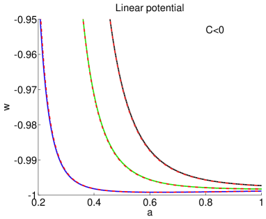
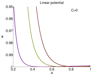
Figure 3: Numerical versus analytic evolution of the equation of state parameter, $w$, for the linear potential. From left to right the plots correspond to $|C|=0.1$, $|C|=0.5$ and $|C|=1$ respectively. The sign of $C$ is indicated on the figure. Solid curves correspond to the exact (numerically-derived) evolution, while the dashed curves indicate the analytical approximation from equations (II) and (17).

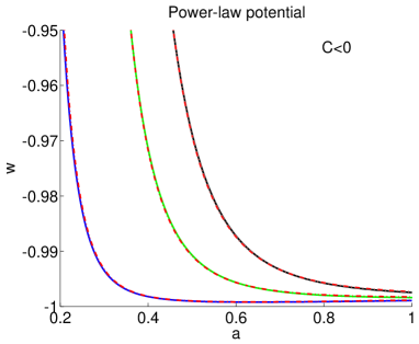
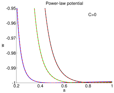
Figure 4: As Fig. 3, for the power-law potential.

Our results are displayed in Figs. 3 and 4. Note that the agreement between our analytic approximation and the true (numerically-calculated) evolution is excellent. This demonstrates that in the regime where the slow roll conditions hold, the evolution of $w$ converges to a common set of tracks irrespective of the details of the underlying quintessence potential.

In the limit where $\lambda=0$, these models correspond to a field evolving in a flat potential, $V=V_{0}$; these models have been dubbed “skating” models Linderpaths . Since we are taking $\lambda\ll 1$, it is reasonable to ask whether the freezing portion of these trajectories can be well-approximated by a pure skating trajectory.

An approximate skating trajectory will be realized whenever the first term in the numerator of equation (8) dominates the second term; this corresponds to the condition

$$1+w\gg\frac{\lambda^{2}}{3}\Omega_{\phi}.$$ (20)

Combining this result with equation (II) (for $C<0$) gives the following condition for the evolution to approximate a skating solution:

$$-C\gg\tanh^{-1}\sqrt{\Omega_{\phi}}-\sqrt{\Omega_{\phi}}.$$ (21)

Equation (21) indicates that, for a given $C$, our models approximate a skating solution at sufficently early times (small $\Omega_{\phi}$). We can demonstrate this explicitly by solving equation (8) for the case $\lambda=0$, giving

$$(1-w)(1+w)\frac{\Omega_{\phi}^{2}}{\left(1-\Omega_{\phi}\right)^{2}}=k,$$ (22)

where $k$ is a constant. At first glance, it is not obvious how equations (22) and (II) could correspond to the same behavior for $w(\Omega_{\phi}$). However, if we take the limit of small $\Omega_{\phi}$ in equation (II), as indicated by equation (21), and take $1+w\ll 1$ in equation (22) (since it is only in this limit that equation (II) will be valid), we see that the two expressions are, in fact, equivalent, with $k$ in equation (22) given by $k=(2/3)\lambda_{0}^{2}C^{2}$.

We explore this equivalence in Fig. 5. Here we plot several $w(a)$ curves for the linear potential, along with the evolution of $w$ for the corresponding pure skating potential. As expected, the two sets of trajectories coincide at early times but diverge at late times. However, since it is the latter which is the epoch of interest observationally, the approximation developed here cannot usefully be replaced by the solution appropriate to a constant potential.

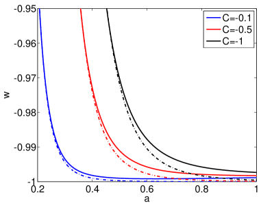
Figure 5: The equation of state parameter, $w$, as a function of the scale factor, $a$, for the linear potential (equation 18) with $\alpha=0.1$ and the indicated values of $C$ (solid curves), along with the corresponding models with $\alpha=0$ (dashed curves).

IV Discussion

We have extended earlier work on nearly flat potentials to include the cases where $\dot{\phi}\neq 0$ initially. In these cases, the single trajectory for $(1+w)/\lambda_{0}^{2}$ as a function of $\Omega_{\phi}$, derived in Ref. ScherrerSen1 , becomes a family of trajectories parametrized by a constant $C$ that depends on the initial value of $\dot{\phi}$. All such trajectories show roughly the same behavior: an initial period of freezing behavior, for which $w$ decreases with time, followed by a thawing period, for which $w$ increases. However, this thawing period can take place in the future, so these models allow for purely freezing behavior up to the present. Note that behavior of this type (with freezing followed by thawing) was also noted in the Monte Carlo simulations of Huterer and Peiris HP , although their space of sampled models differs significantly from the class of models explored here.

Our results differ from the earlier work in Refs. Watson and Chiba , who also examined freezing models. However, these papers assumed a model that began on a tracking trajectory, with $w$ initially constant and far from $-1$, and then examined the freezing evolution as the scalar field began to influence the expansion. The models discussed here assume that the potential is sufficiently flat that $w$ is already close to $-1$ at late times, so we expect very different evolution between these two cases.

The results presented here can be easily generalized, as in Ref. ScherrerSen2 , to phantom models with a negative kinetic term. The result is simply equation (II) multiplied by $-1$ on the right-hand side.

Obviously, our results apply only to a special set of quintessence potentials. However, they do provide an interesting set of restricted evolutionary paths for such potentials, and potentials satisfying the slow-roll conditions are a “natural” way to produce the observed value of $w$ close to $-1$ today. One might argue, in that regard, that the freezing models discussed here are less natural than the thawing models discussed in Ref. ScherrerSen1 . This is a valid criticism, since in the former case one must tune the initial value of $\dot{\phi}$ to give $w$ sufficiently close to $-1$ at present. Furthermore, the evolution discussed here cannot be extrapolated arbitrarily far into the past, since this would result in an early universe dominated by scalar field kinetic energy, in contradiction to observations stiff . Thus, the slow roll conditions on $V(\phi)$ cannot be satisfied at arbitrarily early times; the field must have evolved from a region with a different form for $V(\phi)$, giving a different evolution for $w(a)$ in the early universe. This means that freezing slow-roll models are necessarily more complicated than the thawing models considered in Ref. ScherrerSen1 , which do not have similar problems with their evolution at early times. However, in the absence of any compelling a priori models for the scalar field, it is worthwhile to consider all reasonable possibilities.

V Acknowledgments

R.J.S. was supported in part by the Department of Energy (DE-FG05-85ER40226).

References

- (1) M. Kowalski et al., Astrophys. J. 686, 749 (2008).
- (2) L. Perivolaropoulos and A. Shafieloo, Phys. Rev. D79, 123502 (2009).
- (3) M. Hicken et al., Astrophys. J. 700, 1097 (2009).
- (4) E. Komatsu et al., Astrophys. J. Suppl. 180, 330 (2009).
- (5) D. J. Eisenstein et al., Astrophys. J. 633, 560 (2005).
- (6) W. J. Percival, S. Cole, D. J. Eisenstein, R. C. Nichol, J. A. Peacock, A. C. Pope and A. S. Szalay, Mon. Not. Roy. Astron. Soc. 381, 1053 (2007).
- (7) L. Samushia, G. Chen and B. Ratra, arXiv:0706.1963.
- (8) S. Ettori et al., Astron. Astrophys. 501, 61 (2009).
- (9) Y. Wang, Phys. Rev. D 78, 123532 (2008).
- (10) L. Samushia and B. Ratra, Astrophys. J. 714, 1347 (2010).
- (11) E.J. Copeland, M. Sami, and S. Tsujikawa, Int. J. Mod. Phys. D 15, 1753 (2006).
- (12) W.M. Wood-Vasey, et al., Astrophys. J. 666, 694 (2007).
- (13) T.M. Davis, et al., Astrophys. J. 666, 716 (2007).
- (14) B. Ratra and P. J. E. Peebles, Phys. Rev. D 37, 3406 (1988).
- (15) R. R. Caldwell, R. Dave and P. J. Steinhardt, Phys. Rev. Lett. 80, 1582 (1998).
- (16) A. R. Liddle and R. J. Scherrer, Phys. Rev. D 59, 023509 (1999).
- (17) P. J. Steinhardt, L. M. Wang and I. Zlatev, Phys. Rev. D 59, 123504 (1999).
- (18) R.R. Caldwell, Phys. Lett. B 545, 23 (2002).
- (19) S. M. Carroll, M. Hoffman and M. Trodden, Phys. Rev. D 68, 023509 (2003).
- (20) J. M. Cline, S. Jeon and G. D. Moore, Phys. Rev. D 70, 043543 (2004).
- (21) R. V. Buniy and S. D. H. Hsu, Phys. Lett. B 632, 543 (2006).
- (22) R. V. Buniy, S. D. H. Hsu and B. M. Murray, Phys. Rev. D 74, 063518 (2006).
- (23) P. Creminelli, G. D’Amico, J. Norena and F. Vernizzi, JCAP 0902, 018 (2009)
- (24) Y.F. Cai, E.N. Saridakis, M.R. Setare, and J.Q. Xia, Phys. Rep. 493, 1 (2010).
- (25) R. J. Scherrer and A. A. Sen, Phys. Rev. D 77, 083515 (2008)
- (26) R. R. Caldwell and E. V. Linder, Phys. Rev. Lett. 95, 141301 (2005)
- (27) R. J. Scherrer and A. A. Sen, Phys. Rev. D 78, 067303 (2008)
- (28) S. Dutta and R. J. Scherrer, Phys. Rev. D78, 123525 (2008).
- (29) S. Dutta and R. J. Scherrer, Phys. Lett. B 676, 12 (2009).
- (30) S. Dutta, E. N. Saridakis and R. J. Scherrer, Phys. Rev. D79, 103005 (2009).
- (31) T. Chiba, Phys. Rev. D 79, 083517 (2009)
- (32) C.R. Watson and R.J. Scherrer, Phys. Rev. D68, 123524 (2003).
- (33) R. Crittenden, E. Majerotto, and F. Piazza, Phys. Rev. Lett. 98, 251301 (2007).
- (34) I.P. Neupane and C. Scherer, JCAP 0805, 009 (2008).
- (35) R.N. Cahn, R. de Putter, and E.V. Linder, JCAP 0811, 015 (2008).
- (36) T. Chiba, Phys. Rev. D81, 023515 (2010).
- (37) M. Cortes and E.V. Linder, Phys. Rev. D81, 063004 (2010).
- (38) M. Luo and Q.-P. Su, Comm. Theor. Phys., 54, 186 (2010).
- (39) Z. Huang, J.R. Bond, and L. Kofman, Astrophys. J. 726, 64 (2011).
- (40) C. Csaki, N. Kaloper, and J. Terning, JCAP 0606, 022 (2006).
- (41) M. Sahlén, A.R. Liddle, and D. Parkinson, Phys. Rev. D72, 083511 (2005).
- (42) M. Sahlén, A.R. Liddle, and D. Parkinson, Phys. Rev. D75, 023502 (2007).
- (43) E.V. Linder, Phys. Rev. D73, 063010 (2006).
- (44) D. Huterer and H.V. Peiris, Phys. Rev. D75, 083503 (2007).
- (45) S. Dutta and R.J. Scherrer, Phys. Rev. D82, 083501 (2010).