On the Minimal Length Uncertainty Relation and the Foundations of String Theory

Abstract

We review our work on the minimal length uncertainty relation as suggested by perturbative string theory. We discuss simple phenomenological implications of the minimal length uncertainty relation and then argue that the combination of the principles of quantum theory and general relativity allow for a dynamical energy-momentum space. We discuss the implication of this for the problem of vacuum energy and the foundations of non-perturbative string theory.

I Introduction

One of the unequivocal characteristics of string theory string-textbooks is its possession of a fundamental length scale which determines the typical spacetime extension of a fundamental string. This is $\ell_{s}=\sqrt{\alpha^{\prime}}$, where $\hbar c/\alpha^{\prime}$ is the string tension. Such a feature is to be expected of any candidate theory of quantum gravity, since gravity itself is characterized by the Planck length $\ell_{\mathrm{P}}=\sqrt{\hbar G_{\mathrm{N}}/c^{3}}$. Moreover, $\ell_{\mathrm{P}}\sim\ell_{s}$ is understood to be the minimal length below which spacetime distances cannot be resolved Wheeler:1957mu ; MinimalLength :

$$\delta s\;\gtrsim\;\ell_{\mathrm{P}}\sim\ell_{s}\;.$$ (1)

Quantum theory, on the other hand, is completely oblivious to the presence of such a scale, despite its being the putative infrared limit of string theory. A natural question to ask is, therefore, whether the formalism of quantum theory can be deformed or extended in such a way as to consistently incorporate the minimal length. If it is at all possible, the precise manner in which quantum theory must be modified may point to solutions of yet unresolved mysteries such as the cosmological constant problem CosmoConstant , which is quantum gravitational in its origin. It should also illuminate the nature of string theory joewhat , whence quantum theory must emerge CLMTT .

The idea of introducing a minimal length into quantum theory has a fascinating and long history. It was used by Heisenberg in 1930 kragh to address the infinities of the newly formulated theory of quantum electodynamics Heisenberg:1929xj . Over the years, the idea has been picked up by many authors in a plethora of contexts, e.g. Refs. born:1933 ; Snyder:1946qz ; Yang:1947ud ; Mead:1966zz ; Pavlopoulos:1967dm ; Padmanabhan:1986ny ; Hossenfelder:2003jz ; Das:2008kaa ; Bagchi:2009wb to list just a few. Various ways to deform or extend quantum theory have also been suggested Weinberg:1989cm ; Bender:2002vv . In this paper, we focus our attention on how a minimal length can be introduced into quantum mechanics by modifing its algebraic structure Maggiore:1993zu ; Kempf:1994su .

The starting point of our analysis is the minimal length uncertainty relation (MLUR) Amati:1988tn ,

$$\delta x\;\sim\;\left(\dfrac{\hbar}{\delta p}+\alpha^{\prime}\,\dfrac{\delta p}{\hbar}\right)\;,$$ (2)

which is suggested by a re-summed perturbation expansion of the string-string scattering amplitude in a flat spacetime background gross . This is essentially a Heisenberg microscope argument HeisenbergMicroscope in the S-matrix language Smatrix with fundamental strings used to probe fundamental strings. The first term inside the parentheses on the right-hand side is the usual Heisenberg term coming from the shortening of the probe-wavelength as momentum is increased, while the second-term can be understood as due to the lengthening of the probe string as more energy is pumped into it:

$$\delta p\;=\;\dfrac{\delta E}{c}\;\sim\;\dfrac{\hbar}{\alpha^{\prime}}\,\delta x\;.$$ (3)

Eq. (2) implies that the uncertainty in position, $\delta x$, is bounded from below by the string length scale,

$$\delta x\;\gtrsim\;\sqrt{\alpha^{\prime}}\;=\;\ell_{s}\;,$$ (4)

where the minimum occurs at

$$\delta p\;\sim\;\dfrac{\hbar}{\sqrt{\alpha^{\prime}}}\;=\;\dfrac{\hbar}{\ell_{s}}\;\equiv\;\mu_{s}\;.$$ (5)

Thus, $\ell_{s}$ is the minimal length below which spatial distances cannot be resolved, consistent with Eq. (1). In fact, the MLUR can be motivated by fairly elementary general relativistic considerations independent of string theory, which suggests that it is a universal feature of quantum gravity Wheeler:1957mu ; MinimalLength .

Note that in the trans-Planckian momentum region $\delta p\gg\mu_{s}$, the MLUR is dominated by the behavior of Eq. (3), which implies that large $\delta p$ (UV) corresponds to large $\delta x$ (IR), and that there exists a correspondence between UV and IR physics. Such UV/IR relations have been observed in various string dualities string-textbooks , and in the context of AdS/CFT correspondence uvir (albeit between the bulk and boundary theories). Thus, the MLUR captures another distinguishing feature of string theory.

In addition to the MLUR, another uncertainty relation has been pointed out by Yoneya as characteristic of string theory. This is the so-called spacetime uncertainty relation (STUR)

$$\delta x\,\delta t\;\sim\;\ell_{s}^{2}/c\;,$$ (6)

which can be motivated in a somewhat hand-waving manner by combining the usual energy-time uncertainty relation $\delta E\,\delta t\sim\hbar$ energytimeUR with Eq. (3). However, it can also be supported via an analysis of D0-brane scattering in certain backgrounds in which $\delta x$ can be made arbitrary small at the expense of making the duration of the interaction $\delta t$ arbitrary large yoneya . While the MLUR pertains to dynamics of a particle in a non-dynamic spacetime, the STUR can be interpreted to pertain to the dynamics of spacetime itself in which the size of a quantized spacetime cell is preserved.

In the following, we discuss how the MLUR and STUR may be incorporated into quantum mechanics via a deformation and/or extension of its algebraic structure. In section II, we introduce a deformation of the canonical commutation relation between $\hat{x}$ and $\hat{p}$ which leads to the MLUR, and discuss its phenomenological consequences. In section III, we take the classical limit by replacing commutation relations with Poisson brackets and derive the analogue of Liouville’s theorem in the deformed mechanics. We then discuss the effect this has on the density of states in phase space. In section IV, we discuss the implications of the MLUR on the cosmological constant problem. We conclude in section V with some speculations on how the STUR may be incorporated via a Nambu triple bracket, and comment on the lessons for the foundations of string theory and on the question “What is string theory?”

II Quantum Mechanical Model of the Minimal Length

II.1 Deformed Commutation Relations

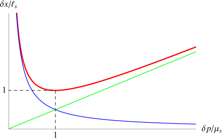
Figure 1: The $\delta p$-dependence of the lower bound of $\delta x$ under the minimal length uncertainty relation Eq. (7) (red curve). The bound for the usual Heisenberg relation $\delta x\geq\hbar/(2\delta p)$ is shown in blue, and the linear bound $\delta x\geq(\hbar\beta/2)\delta p$ is shown in green.

To place the MLUR, Eq. (2), on firmer ground, we begin by rewriting it as

$$\delta x\,\delta p\;\geq\;\dfrac{\hbar}{2}\left(1+\beta\,{\delta p}^{2}\right)\;,$$ (7)

where we have introduced the parameter $\beta=\alpha^{\prime}/\hbar^{2}$. The minimum value of $\delta x$ as a function of $\delta p$ is plotted in Fig. 1. This uncertainty relation can be reproduced by deforming the canonical commutation relation between $\hat{x}$ and $\hat{p}$ to:

$$\dfrac{1}{i\hbar}\left[\,\hat{x},\,\hat{p}\,\right]\;=\;1\qquad\longrightarrow\qquad\dfrac{1}{i\hbar}\left[\,\hat{x},\,\hat{p}\,\right]\;=\;A(\hat{p}^{2})\;,$$ (8)

with $A(p^{2})=1+\beta p^{2}$. Indeed, we find

$$\delta x\,\delta p\;\geq\;\dfrac{1}{2}\Bigl{|}\bigl{\langle}\left[\,\hat{x},\,\hat{p}\,\right]\bigr{\rangle}\Bigr{|}\;=\;\dfrac{\hbar}{2}\left(1+\beta\left\langle\hat{p}^{2}\right\rangle\right)\;\geq\;\dfrac{\hbar}{2}\left(1+\beta\,\delta p^{2}\right)\;,$$ (9)

since $\delta p^{2}=\left\langle\hat{p}^{2}\right\rangle-\left\langle\hat{p}\right\rangle^{2}$. The function $A(p^{2})$ can actually be more generic, with $\beta p^{2}$ being the linear term in its expansion in $p^{2}$.

When we have more than one spatial dimension, the above commutation relation can be generalized to

$$\dfrac{1}{i\hbar}[\,\hat{x}_{i},\,\hat{p}_{j}\,]\;=\;A(\hat{\mathbf{p}}^{2})\,\delta_{ij}+B(\hat{\mathbf{p}}^{2})\,\hat{p}_{i}\hat{p}_{j}\;,$$ (10)

where $\hat{\mathbf{p}}^{2}=\sum_{i}\hat{p}_{i}^{2}$. The right-hand side is the most general form that depends only on the momentum and respects rotational symmetry. Assuming that the components of the momentum commute among themselves,

$$[\,\hat{p}_{i},\,\hat{p}_{j}\,]\;=\;0\;,$$ (11)

the Jacobi identity demands that

$$\dfrac{1}{i\hbar}[\,\hat{x}_{i},\,\hat{x}_{j}\,]\;=\;-\left\{\,2(\hat{A}+\hat{B}\hat{\mathbf{p}}^{2})\hat{A}^{\prime}-\hat{A}\hat{B}\,\right\}\hat{L}_{ij}\;,$$ (12)

where we have used the shorthand $\hat{A}=A(\hat{\mathbf{p}}^{2})$, $\hat{A}^{\prime}=\dfrac{dA}{d\mathbf{p}^{2}}(\hat{\mathbf{p}}^{2})$, $\hat{B}=B(\hat{\mathbf{p}}^{2})$, and $\hat{L}_{ij}=\left(\hat{x}_{i}\hat{p}_{j}-\hat{x}_{j}\hat{p}_{i}\right)/\hat{A}$ . That $\hat{L}_{ij}$ generates rotations can be seen from the following:

$$\dfrac{1}{i\hbar}[\,\hat{L}_{ij}\,\hat{x}_{k}\,] = \delta_{ik}\hat{x}_{j}-\delta_{jk}\hat{x}_{i}\;,$$ (13)

$$\dfrac{1}{i\hbar}[\,\hat{L}_{ij}\,\hat{p}_{k}\,] = \delta_{ik}\hat{p}_{j}-\delta_{jk}\hat{p}_{i}\;,$$ (14)

$$\dfrac{1}{i\hbar}[\,\hat{L}_{ij}\,\hat{L}_{k\ell}\,] = \delta_{ik}\hat{L}_{j\ell}-\delta_{i\ell}\hat{L}_{jk}+\delta_{j\ell}\hat{L}_{ik}-\delta_{jk}\hat{L}_{i\ell}\;.$$ (15)

Note that the non-commutativity of the components of position can be interpreted as a reflection of the dynamic nature of space itself, as would be expected in quantum gravity.

Various choices for the functions $A(\mathbf{p}^{2})$ and $B(\mathbf{p}^{2})$ have been considered in the literature. Maggiore Maggiore:1993zu proposed

$$A(\mathbf{p}^{2})\;=\;\sqrt{1+2\beta\mathbf{p}^{2}}\;,\qquad B(\mathbf{p}^{2})\;=\;0\;,\qquad\dfrac{1}{i\hbar}[\,\hat{x}_{i},\,\hat{x}_{j}\,]\;=\;-2\beta\hat{L}_{ij}\;,$$ (16)

while Kempf Kempf:1994su assumed

$$A(\mathbf{p}^{2})\;=\;1+\beta\mathbf{p}^{2}\;,\qquad B(\mathbf{p}^{2})\;=\;\beta^{\prime}\;=\;\mathrm{constant}\;,$$ (17)

in which case

$$\dfrac{1}{i\hbar}[\,\hat{x}_{i},\,\hat{x}_{j}\,]\;=\;-\left\{\,(2\beta-\beta^{\prime})+\beta(2\beta+\beta^{\prime})\hat{\mathbf{p}}^{2}\right\}\hat{L}_{ij}\;.$$ (18)

Kempf’s choice encompasses the algebra of Snyder Snyder:1946qz

$$A(\mathbf{p}^{2})\;=\;1\;,\qquad B(\mathbf{p}^{2})\;=\;\beta^{\prime}\;,\qquad\dfrac{1}{i\hbar}[\,\hat{x}_{i},\,\hat{x}_{j}\,]\;=\;\beta^{\prime}\hat{L}_{ij}\;,$$ (19)

and that of Brau Brau:1999uv ; Brau:2006ca

$$A(\mathbf{p}^{2})\;=\;1+\beta\mathbf{p}^{2}\;,\qquad B(\mathbf{p}^{2})\;=\;2\beta\;,\qquad\dfrac{1}{i\hbar}[\,\hat{x}_{i},\,\hat{x}_{j}\,]\;=\;O(\beta^{2})\;,$$ (20)

for which the components of the position approximately commute. In our treatment, we follow Kempf and use Eq. (17).

II.2 Shifts in the Energy Levels

Let us see whether the above deformed commutation relations lead to a reasonable quantum mechanics, with well defined energy eigenvalues and eigenstates. Given a Hamiltonian in terms of the deformed position and momentum operators, $H(\hat{\mathbf{x}},\hat{\mathbf{p}})$, we would like to solve the time-independent Schrödinger equation

$$H(\hat{\mathbf{x}},\hat{\mathbf{p}})\,|E\rangle\;=\;E\,|E\rangle\;.$$ (21)

The operators which satisfy Eqs. (10), (11), and (12), subject to the choice Eq. (17), can be represented using operators which obey the canonical commutation relation $[\,\hat{q}_{i},\,\hat{p}_{j}\,]=i\hbar\,\delta_{ij}$ as Kempf:1994su ; Benczik:2007we

$$\hat{x}_{i} = \hat{q}_{i}+\beta\;\dfrac{\hat{p}^{2}\hat{q}_{i}+\hat{q}_{i}\,\hat{p}^{2}}{2}+\beta^{\prime}\,\dfrac{\hat{p}_{i}\,(\hat{p}\cdot\hat{q})+(\hat{q}\cdot\hat{p})\,\hat{p}_{i}}{2}\;,$$ (22)

$$\hat{p}_{i} = \hat{p}_{i}\;.$$ (23)

The $\beta$ and $\beta^{\prime}$ terms are symmetrized to ensure the hermiticity of $\hat{x}_{i}$. Note that this representation allows us to write the Hamiltonian in terms of canonical $\hat{q}_{i}$’s and $\hat{p}_{i}$’s:

$$H^{\prime}(\hat{\mathbf{q}},\hat{\mathbf{p}})\;\equiv\;H(\hat{\mathbf{x}}(\hat{\mathbf{q}},\hat{\mathbf{p}}),\hat{\mathbf{p}})\;.$$ (24)

Thus, our deformation of the canonical commutation relations is mathematically equivalent to a deformation of the Hamiltonian.

By the standard replacements

$$\hat{q}_{i}\;=\;q_{i}\;,\quad\hat{p}_{i}\;=\;\dfrac{\hbar}{i}\dfrac{\partial}{\partial q_{i}}\;,\qquad\mbox{or}\qquad\hat{q}_{i}\;=\;i\hbar\dfrac{\partial}{\partial p_{i}}\;,\quad\hat{p}_{i}\;=\;p_{i}\;,$$ (25)

$\hat{x}_{i}$ and $\hat{p}_{j}$ can be represented as differential operators acting on a Hilbert space of $L^{2}$ functions in either the $q_{i}$’s or the $p_{i}$’s, and one can write down a Schrödinger equation for a given Hamiltonian in either $q$-space or $p$-space to solve for the energy eigenvalues. Note, however, that while the $p_{i}$’s are the eigenvalues of the momentum operators $\hat{p}_{i}$, the $q_{i}$’s are not the eigenvalues of the position operator $\hat{x}_{i}$. In fact, the existence of the minimal length implies that $\hat{x}_{i}$ cannot have any eigenfunctions within either Hilbert spaces. Therefore, the meaning of the wave-function in $q$-space is somewhat ambiguous. Nevertheless, the $q$-space representation is particularly useful when the Schrödinger equation cannot be solved exactly, since one can treat

$$\Delta H(\hat{\mathbf{q}},\hat{\mathbf{p}})\;=\;H^{\prime}(\hat{\mathbf{q}},\hat{\mathbf{p}})-H(\hat{\mathbf{q}},\hat{\mathbf{p}})$$ (26)

as a perturbation and calculate the shifts in the energies via perturbation theory in $q$-space.

In the following, we look at the energy shifts induced by non-zero $\beta$ and $\beta^{\prime}$ in the harmonic oscillator Kempf:1996fz ; Chang:2001kn , the Hydrogen atom Brau:1999uv ; Benczik:2005bh , and a particle in a uniform gravitational well Benczik:2007we ; Brau:2006ca . Since detailed derivations can be found in the respective references, we only provide an outline of the results in each case.

II.2.1 Harmonic Oscillator

Consider a $D$-dimensional isotropic harmonic oscillator. The Hamiltonian is of course

$$\hat{H}\;=\;\dfrac{\hat{\mathbf{p}}^{2}}{2m}+\dfrac{1}{2}m\omega^{2}\hat{\mathbf{x}}^{2}\;.$$ (27)

The $p$-space representation of the operators are

$$\hat{x}_{i} = i\hbar\left[(1+\beta p^{2})\frac{\partial}{\partial p_{i}}+\beta^{\prime}p_{i}p_{j}\frac{\partial}{\partial p_{j}}+\left\{\beta+\beta^{\prime}\left(\dfrac{D+1}{2}\right)-\delta(\beta+\beta^{\prime})\right\}\,p_{i}\right]\;,$$ (28)

$$\hat{p}_{i} = p_{i}\;.$$ (29)

Here, $\delta$ is an arbitrary real parameter which can be used to simplify the representation of the operator $\hat{x}_{i}$ at the expense of modifying the definition of the inner product in $p$-space to

$$\langle f|g\rangle_{\delta}\;=\;\int\dfrac{d^{D}\mathbf{p}}{[\,1+(\beta+\beta^{\prime})\mathbf{p}^{2}\,]^{\delta}}\;f^{*}(\mathbf{p})\,g(\mathbf{p})\;.$$ (30)

The introduction of $\delta$ is a canonical transformation which does not affect the energy eigenvalues Benczik:2007we . The choice

$$\delta\;=\;\dfrac{\beta+\beta^{\prime}\left(\dfrac{D+1}{2}\right)}{\beta+\beta^{\prime}}$$ (31)

eliminates the third term in the expression for $\hat{x}_{i}$.

The rotational symmetry of the Hamiltonian, Eq. (27), allows us to write the wave-function in $p$-space as a product of a radial wave-function and a $D$-dimensional spherical harmonic:

$$\Psi_{D}(\mathbf{p})\;=\;R(p)\,Y_{\ell\,m_{D-2}m_{D-3}\cdots m_{2}m_{1}}(\Omega)\;,\qquad p\;\equiv\;|\mathbf{p}|\;.$$ (32)

The radial Schrödinger equation is then

$$-m\hbar\omega\Biggl{[}\left\{\Bigl{[}1+(\beta+\beta^{\prime})p^{2}\Bigr{]}\frac{\partial}{\partial p}\right\}^{2}+\frac{(D-1)(1+\beta\,p^{2})[1+(\beta+\beta^{\prime})p^{2}]}{p}\frac{\partial}{\partial p}$$ (33)

$$\hskip 142.26378pt-\frac{L^{2}(1+\beta\,p^{2})^{2}}{p^{2}}\Biggr{]}\,R(p)+\frac{1}{m\hbar\omega}\,p^{2}\,R(p)\;=\;\frac{2E}{\hbar\omega}\,R(p)\;,$$ (34)

where

$$L^{2}\;=\;\ell(\ell+D-2)\;,\qquad\ell\;=\;0,1,2,\cdots$$ (35)

is the eigenvalue of the angular momentum operator in $D$-dimensions. The solution to Eq. (34) has been worked out in detail in Ref. Chang:2001kn , and the energy eigenvalues are

$$E_{n\ell} = \hbar\omega\left[\left(n+\frac{D}{2}\right)\sqrt{1+\left\{\beta^{2}L^{2}+\frac{(D\beta+\beta^{\prime})^{2}}{4}\right\}m^{2}\hbar^{2}\omega^{2}}\right.$$ (37)

$$\qquad\left.+\left\{(\beta+\beta^{\prime})\left(n+\frac{D}{2}\right)^{2}+(\beta-\beta^{\prime})\left(L^{2}+\frac{D^{2}}{4}\right)+\beta^{\prime}\frac{D}{2}\right\}\frac{m\hbar\omega}{2}\right]\;,$$

with eigenfunctions given by

$$R_{n\ell}(p)\;=\;(\beta+\beta^{\prime})^{D/4}\sqrt{\dfrac{2(2k+a+b+1)\,k!\,\Gamma(k+a+b+1)}{\Gamma(k+a+1)\Gamma(k+b+1)}}\;\left(\dfrac{1-z}{2}\right)^{\lambda/2}\left(\dfrac{1+z}{2}\right)^{\ell/2}P_{k}^{(a,b)}(z)\;.$$ (38)

Here, $P_{k}^{(a,b)}(z)$ is the Jacobi polynomial of order $k=(n-\ell)/2$ with argument

$$z\;=\;\dfrac{(\beta+\beta^{\prime})p^{2}-1}{(\beta+\beta^{\prime})p^{2}+1}\;,$$ (39)

and

$$a\;=\;\dfrac{1}{m\hbar\omega(\beta+\beta^{\prime})}\sqrt{1+\left\{\beta^{2}L^{2}+\dfrac{(D\beta+\beta^{\prime})^{2}}{4}\right\}m^{2}\hbar^{2}\omega^{2}}\;,\qquad b\;=\;\frac{D}{2}+\ell-1\;,\qquad\lambda\;=\;\frac{D\beta+\beta^{\prime}}{2(\beta+\beta^{\prime})}+a\;.$$ (40)

Note that due to the $(n+D/2)^{2}$ dependend term in Eq. (37), the energy levels are no longer uniformly spaced. Note also, that due to the explicit $L^{2}$-dependence, the original

$$\frac{(D+n-1)!}{(D-1)!\,n!}$$ (41)

fold degeneracy of the $n$-th energy level, which was due to states with different $k$ and $\ell$ sharing the same $n=2k+\ell$, is resolved, leaving only the

$$\frac{(D+\ell-1)!}{(D-1)!\,\ell!}-\frac{(D+\ell-3)!}{(D-1)!\,(\ell-2)!}$$ (42)

fold degeneracy for each value of $\ell$ due to rotational symmetry alone Chodos:1983zi . For example, in $D=2$ dimensions, the $(n+1)$-fold degeneracy of the $n$-th level breaks down to the 2-fold degeneracies between the pairs of $m=\pm\ell$ states. This is illustrated in Fig. 2

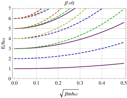
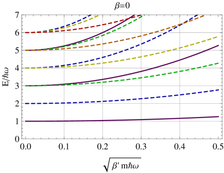
Figure 2: The energy levels of the 2D isotropic harmonic oscillator for the cases $\beta^{\prime}=0$ (left) and $\beta=0$ (right). The purple solid lines indicate $s$-wave states which are singlets. The dashed lines are doublets with the color indicating $\ell=1$ (blue), $\ell=2$ (green), $\ell=3$ (yellow), $\ell=4$ (orange), and $\ell=5$ (red). $\sqrt{\beta m\hbar\omega}$ is the ratio of the minimal length $\hbar\sqrt{\beta}$ to the characteristic length scale $\sqrt{\hbar/m\omega}$ of the system.

II.2.2 Hydrogen Atom

The introduction of a minimal length to the Coulomb potential problem was first discussed by Born in 1933 born:1933 . There, it was argued that the singularity at $r=0$ will be blurred out. Here, we find a similar effect. We consider the usual Hydrogen atom Hamiltonian in $D$-dimensions:

$$\hat{H}\;=\;\dfrac{\hat{\mathbf{p}}^{2}}{2m}-\dfrac{e^{2}}{\hat{r}}\;,$$ (43)

where the operator $1/\hat{r}$ is defined as the inverse of the square-root of the operator

$$\hat{r}^{2}\;=\;\sum_{i=1}^{D}\hat{x}_{i}^{2}\;.$$ (44)

$1/\hat{r}$ will be best represented in the basis in which $\hat{r}^{2}$ is diagonal. The eigenvalues of $\hat{r}^{2}$ can be obtained from those of the harmonic oscillator, Eq. (37), by taking the limit $m\rightarrow\infty$:

$$r_{k\ell}^{2} = \lim_{m\rightarrow\infty}\dfrac{2E_{n\ell}}{m\omega^{2}}$$ (45)

$$= \hbar^{2}(\beta+\beta^{\prime})\left[\left\{\left(2k+\ell+\dfrac{D}{2}\right)+\dfrac{1}{\beta+\beta^{\prime}}\sqrt{\beta^{2}L^{2}+\dfrac{(D\beta+\beta^{\prime})^{2}}{4}}\right\}^{2}-\dfrac{\beta^{\prime}}{\beta+\beta^{\prime}}\Biggl{\{}L^{2}+\dfrac{(D-1)^{2}}{4}\Biggr{\}}\right]\;.$$ (46)

The corresponding eigenfunctions are given by the same expression as Eq. (38) except with $a$ replaced by

$$a\;=\;\dfrac{1}{\beta+\beta^{\prime}}\sqrt{\beta^{2}L^{2}+\dfrac{(D\beta+\beta^{\prime})^{2}}{4}}\;.$$ (47)

Denoting these eigenfunctions as $R_{k\ell}(p)$, we can define

$$\dfrac{1}{\hat{r}}\,R_{k\ell}(p)\;=\;\dfrac{1}{r_{k\ell}}\,R_{k\ell}(p)\;.$$ (48)

As in the harmonic oscillator case, the rotational symmetry of the Hamiltonian allows us to write an energy eigenstate wave-function as a product of a radial wave-function and a spherical harmonic. The radial wave-function can then be expressed as a superposition of the $\hat{r}^{2}$ eigenfunctions with fixed $\ell$:

$$R_{\ell}(p)\;=\;\sum_{k=0}^{\infty}f_{k}R_{k\ell}(p)\;.$$ (49)

The radial Schrödinger equation will impose a recursion relation on the coefficients $f_{n}$, which can be solved numerically on a computer. The condition that the resulting function be square-integrable determines the eigenvalues $E$. The detailed procedure can be found in Ref. Benczik:2005bh ; Benczik:2007we . Here, we only display the results for the $D=3$ case in Fig. 3. As can be seen, the degeneracy between difference angular momentum states are lifted, just as in the harmonic oscillator case.

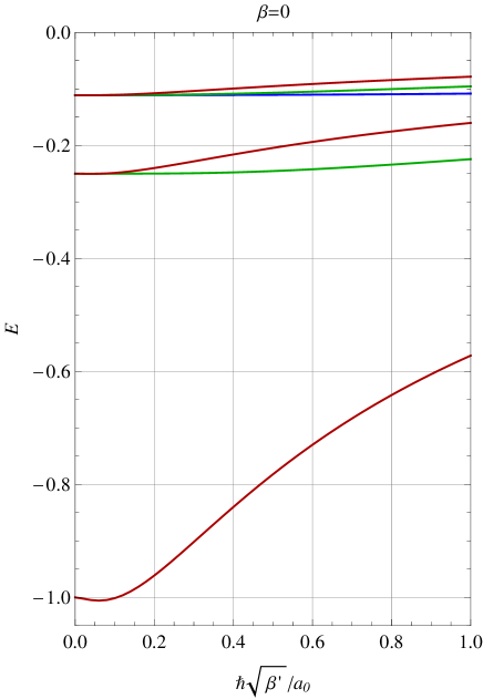
Figure 3: Energy shifts of the $n=1$, $2$, and $3$ states of the Hydrogen atom for the $\beta^{\prime}=0$ (left) and $\beta=0$ (right) cases. $a_{0}=\hbar^{2}/me^{2}$ is the Bohr radius and the energy is in units of the Rydberg constant $e^{2}/2a_{0}$. The color of the lines indicate the orbital angular momentum: $s$ (red), $p$ (green), and $d$ (blue). The $s$-wave states are affected non-perturbatively even for very small $\beta$ or $\beta^{\prime}$, indicating their sensitivity to the singularity of the Coulomb potential at the origin.

It is also possible to calculate the energy shifts perturbatively using the $q$-space representation for the cases $D\geq 4$ or $\ell\neq 0$. The unperturbed energy eigenfunctions in $D$-dimensions are

$$R_{n\ell}(q)\;=\;\sqrt{\dfrac{2^{2D}}{a_{0}^{D}\left(2n+D-3\right)^{D+1}}\,\dfrac{(n-\ell-1)!}{(n+\ell+D-3)!}}\;e^{-\rho/2}\rho^{\ell}L_{n-\ell-1}^{(2\ell+D-2)}(\rho)\;,$$ (50)

where $a_{0}=\hbar^{2}/me^{2}$ is the Bohr radius, $L_{k}^{(\lambda)}(\rho)$ the order $k$ Laguerre polynomial, and

$$\rho\;=\;\dfrac{2q}{a_{0}\left(n+\frac{D-3}{2}\right)}\;.$$ (51)

The eigenvalues are

$$E_{n}\;=\;-\dfrac{e^{2}}{2a_{0}\left(n+\frac{D-3}{2}\right)^{2}}\;,\qquad\qquad n\,=\,1,\,2,\,3,\cdots$$ (52)

The operator $1/\hat{r}$ can be expanded in powers of $\beta$ and $\beta^{\prime}$ as Benczik:2007we

$$\dfrac{1}{\hat{r}}\;=\;\dfrac{1}{q}+\hbar^{2}\beta\left(\dfrac{1}{q}\dfrac{\partial^{2}}{\partial q^{2}}+\dfrac{D-2}{q^{2}}\dfrac{\partial}{\partial q}-\dfrac{L^{2}+D-2}{q^{3}}\right)+\hbar^{2}\beta^{\prime}\left(\dfrac{1}{q}\dfrac{\partial^{2}}{\partial q^{2}}+\dfrac{D-2}{q^{2}}\dfrac{\partial}{\partial q}+\dfrac{D^{2}-5D+8}{4q^{3}}\right)+\cdots\;,$$ (53)

and the expectation value of the extra terms converges for $\ell\neq 0$ or $D\geq 4$, yielding

$$\Delta E_{n\ell}\;=\;\dfrac{e^{2}}{a_{0}\left(n+\frac{D-3}{2}\right){}^{3}}\;\dfrac{\hbar^{2}}{a_{0}^{2}}\!\left[\dfrac{(D-1)(2\beta-\beta^{\prime})}{4\left(\ell+\frac{D-3}{2}\right)\left(\ell+\frac{D-2}{2}\right)\left(\ell+\frac{D-1}{2}\right)}+\dfrac{(2\beta+\beta^{\prime})}{\left(\ell+\frac{D-2}{2}\right)}-\dfrac{(\beta+\beta^{\prime})}{\left(n+\frac{D-3}{2}\right)}\right]\;,$$ (54)

which agrees very well with the numerical results for all cases to which it is applicable. For $D=3$, this formula reduces to

$$\Delta E_{n\ell}\;=\;\dfrac{e^{2}}{a_{0}n^{3}}\;\dfrac{\hbar^{2}}{a_{0}^{2}}\!\left[\dfrac{(2\beta-\beta^{\prime})}{2\,\ell\left(\ell+\frac{1}{2}\right)\left(\ell+1\right)}+\dfrac{(2\beta+\beta^{\prime})}{\left(\ell+\frac{1}{2}\right)}-\dfrac{(\beta+\beta^{\prime})}{n}\right]\;,$$ (55)

which is clearly problematic for $\ell=0$. This is due to the breakdown of the expansion Eq. (53) near $q=0$ for $D\leq 3$. Physically, this can be interpreted to mean that the $s$-wave in 3D and lower dimensions is sensitive to the non-perturbative resolution of the singularity at the origin due to the minimal length. Interestingly, in 4D and higher, there are enough spatial dimensions for the wave-function to spread out around the origin so that even the $s$-wave is insensitive to the singularity, and the effect of the minimal length becomes perturbative.

II.2.3 Uniform Gravitational Potential

This subsection is based on unpublished material by Benczik in Ref. Benczik:2007we . Consider the 1D motion of a particle in a linear potential

$$V(x)\;=\;\left\{\begin{array}[]{ll}mgx&x\;>\;0\;,\\ \infty&x\;\leq\;0\;.\end{array}\right.$$ (56)

The Hamiltonian is

$$\hat{H}\;=\;\dfrac{\hat{p}^{2}}{2m}+mg\,\hat{x}\;.$$ (57)

Since $\hat{x}$ does not have any eigenstates within the Hilbert space, the condition $x>0$ is replaced by $\left\langle\hat{x}\right\rangle>0$. In the $q$-space representation, the operators are given by

$$\hat{x} = q\left(1-\hbar^{2}\beta\dfrac{d^{2}}{dq^{2}}\right)\;,$$ (58)

$$\hat{p} = \dfrac{\hbar}{i}\,\dfrac{d}{dq}\;,$$ (59)

and the Schrödinger equation becomes

$$\hat{H}\psi\;=\;-\dfrac{\hbar^{2}}{2m}\,\dfrac{d^{2}\psi}{dq^{2}}+mg\,q\left(1-\hbar^{2}\beta\dfrac{d^{2}}{dq^{2}}\right)\psi\;=\;E\,\psi\;.$$ (60)

The condition $\left\langle\hat{x}\right\rangle>0$ can be imposed by restricting the domain of $q$ to $q>0$, and demanding that the wave function vanish at $q=0$. The solution to the $\beta=0$ case is given by the Airy function

$$\psi_{n}(q)\;=\;\dfrac{1}{|\mathrm{Ai}^{\prime}(\alpha_{n})|}\;\mathrm{Ai}\left(\dfrac{q}{a}+\alpha_{n}\right)\;,\qquad\qquad a\,=\,\left[\dfrac{\hbar^{2}}{2m^{2}g}\right]^{1/3}\;,$$ (61)

with eigenvalues

$$\dfrac{E_{n}}{mga}\;=\;-\alpha_{n}\;,$$ (62)

where

$$\cdots\;<\;\alpha_{3}\;<\;\alpha_{2}\;<\;\alpha_{1}\;<\;0$$ (63)

are the zeroes of $\mathrm{Ai}(z)$. The solution to the $\beta\neq 0$ case is given in terms of the confluent hypergeometric function of the second kind Ufunction :

$$\psi(q)\;\propto\;e^{-q/b}\;U\left(-\dfrac{1}{2}\!\left[\dfrac{E}{mgb}+\dfrac{a^{3}}{b^{3}}\right];\,0\,;\,2\!\left[\dfrac{a^{3}}{b^{3}}+\dfrac{q}{b}\right]\,\right)\;,\qquad a\,=\,\left[\dfrac{\hbar^{2}}{2m^{2}g}\right]^{1/3}\;,\quad b\,=\,\hbar\sqrt{\beta}\;.$$ (64)

The energy eigenvalues are determined by the condition

$$U\left(-\dfrac{1}{2}\!\left[\dfrac{E}{mgb}+\dfrac{a^{3}}{b^{3}}\right];\,0\,;\,\dfrac{2a^{3}}{b^{3}}\,\right)\;=\;0\;,$$ (65)

which can be solved numerically using Mathematica. In Fig. 4, we plot the $b$-dependence of the energies of the lowest lying states. The energies of higher-dimensional cases, in which there are one or more spatial dimensions orthogonal to the potential direction, are discussed in Ref. Benczik:2007we ; Brau:2006ca .

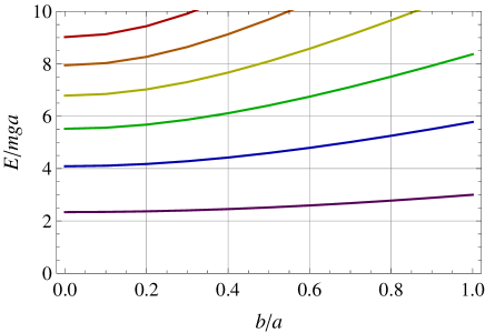
Figure 4: The $b$-dependence of the lowest energy levels of a particle of mass $m$ in a linear gravitaional potential $V(x)=mgx$ with $x>0$. $a=[\hbar^{2}/2m^{2}g]^{1/3}$ is the characteristic length scale of the system, and $b=\hbar\sqrt{\beta}$ is the minimal length.

II.3 Experimental Constraints

As these three examples show, the main effect of the introduction of the minimal length into quantum mechanical systems is the shifts in energy levels which also leads to the breaking of well known degeneracies. The natural question arises whether these shifts can be used to constrain the minimal length experimentally. Of course, if the minimal length is at the Planck scale, detecting its actual effect would be impossible. However, the exercise is of interest to models of large extra dimensions which possess a much lower effective Planck scale than the 4D value LargeExtraDimensions .

In the case of the harmonic oscillator, actual physical systems are never completely harmonic, so it is difficult to distinguish the shift in energy due to anharmonicity with that due to a possible minimal length. Ref. Chang:2001kn considers using the energy levels of an electron in a Penning trap to constrain $\beta$, and finds that even under highly optimistic and unrealistic assumptions, the best bound that can be hoped for is

$$\dfrac{1}{\sqrt{\beta}}\;\gtrsim\;1\;\mathrm{GeV}/c\;.$$ (66)

Refs. Benczik:2007we ; Benczik:2005bh consider placing a bound on $\beta$ using the $1S$ Lamb shift of the Hydrogen atom. The current best experimental value is that given by Schwob et al. in Schwob:1999zz :

$$L_{1s}^{\mathrm{exp}}\;=\;8172.837(22)\;\mathrm{MHz}\;.$$ (67)

This is to be compared with the theoretical value, for which we use that given in Ref. Mallampalli:1998zza :

$$L_{1s}^{\mathrm{th}}\;=\;8172.731(40)\;\mathrm{MHz}\;.$$ (68)

The calculation requires the experimentally determined proton rms charge radius $r_{p}$ as an input, and the error on $L_{1s}^{\mathrm{th}}$ is dominated by the experimental error on $r_{p}$. Here, the value of $r_{p}=0.862(12)\;\mathrm{fm}$ Simon:1980hu was used. Attributing the entire discrepancy to $\beta$ ($\beta^{\prime}=0$), Refs. Benczik:2007we ; Benczik:2005bh cite:

$$\dfrac{1}{\sqrt{\beta}}\;\gtrsim\;7\,\mathrm{GeV}/c\;,$$ (69)

which is only slightly better than Eq. (66). The is no bound on $\beta^{\prime}$ ($\beta=0$) since the shift is in the wrong direction as can be seen in Fig. (3).

The energy levels of neutrons in a linear gravitational potential have been measured by Nesvizhevsky et al. Nesvizhevsky:2002ef . However, as analyzed by Brau and Buisseret Brau:2006ca , the experimental precision is still very many orders of magnitude above what is necessary to place a meaningful bound on $\beta$. The current lower bound on $1/\sqrt{\beta}$ is on the order of $100\,\mathrm{eV}/c$.

III Classical Limit – The Liouville Theorem and the Density of States

Note that rewriting our 1D deformed commutator as

$$[\,\hat{x},\,\hat{p}\,]\;=\;i\hbar A(\hat{p}^{2})$$ (70)

suggests that $\hbar A(p^{2})$ takes on the role of a momentum dependent Planck constant. Given that $\hbar$ determines the size of a quantum mechanical state in phase space, a momentum dependent $\hbar$ would imply that the size of this state must scale according to $A(p^{2})$ as it evolves. To see whether this interpretation makes sense, we formally take the naive classical limit by replacing commutators with Poisson brackets,

$$\dfrac{1}{i\hbar}[\,\hat{x},\,\hat{p}\,]\;=\;A(\hat{p}^{2})\qquad\longrightarrow\qquad\{\,x,\,p\,\}\;=\;A(p^{2})\;,$$ (71)

and proceed to derive the analogue of Liouville’s theorem Chang:2001bm . The Poisson brackets among the $x_{i}$’s and $p_{i}$’s for the multidimensional case are

$$\{\,x_{i},\,p_{j}\,\} = A\,\delta_{ij}+B\,p_{i}p_{j}\;,$$ (72)

$$\{\,p_{i},\,p_{j}\,\} = 0\;,$$ (73)

$$\{\,x_{i},\,x_{j}\,\} = -\left[\dfrac{2(A+B\,\mathbf{p}^{2})}{A}\,\dfrac{dA\;}{d\mathbf{p}^{2}}-B\right]\left(x_{i}p_{j}-x_{j}p_{i}\right)\;.$$ (74)

The generic Poisson bracket of arbitrary functions of the coordinates and momenta can then be defined as

$$\{F,G\}=\left(\frac{\partial F}{\partial x_{i}}\frac{\partial G}{\partial p_{j}}-\frac{\partial F}{\partial p_{i}}\frac{\partial G}{\partial x_{j}}\right)\{x_{i},p_{j}\}+\frac{\partial F}{\partial x_{i}}\frac{\partial G}{\partial x_{j}}\{x_{i},x_{j}\}\;.$$ (75)

Here, we use the convention that repeated indices are summed. Assuming that the equations of motion of $x_{i}$ and $p_{i}$ are given formally by:

$$\dot{x}_{i} = \{\,x_{i},\,H\,\}\;=\;\phantom{-}\{\,x_{i},\,p_{j}\,\}\dfrac{\partial H}{\partial p_{j}}+\{\,x_{i},\,x_{j}\,\}\dfrac{\partial H}{\partial x_{j}}\;,$$ (76)

$$\dot{p}_{i} = \{\,p_{i},\,H\,\}\;=\;-\{\,x_{j},\,p_{i}\,\}\dfrac{\partial H}{\partial x_{j}}\;,$$ (77)

the evolution of $x_{i}$ and $p_{i}$ during an infinitesimal time interval $\delta t$ is found to be:

$$x^{\prime}_{i} = x_{i}+\dot{x}_{i}\,\delta t\;=\;x_{i}+\left[\{\,x_{i},\,p_{j}\,\}\dfrac{\partial H}{\partial p_{j}}+\{\,x_{i},\,x_{j}\,\}\dfrac{\partial H}{\partial x_{j}}\right]\delta t\;,$$ (78)

$$p^{\prime}_{i} = p_{i}+\dot{p}_{i}\,\delta t\;=\;p_{i}-\{\,x_{j},\,p_{i}\,\}\dfrac{\partial H}{\partial x_{j}}\delta t\;.$$ (79)

To find the change in phase space volume associated with this evolution, we calculate the Jacobian of the transformation from $(x_{1},x_{2},\cdots,x_{D};p_{1},p_{2},\cdots,p_{D})$ to $(x^{\prime}_{1},x^{\prime}_{2},\cdots,x^{\prime}_{D};p^{\prime}_{1},p^{\prime}_{2},\cdots,p^{\prime}_{D})$:

$$d^{D}\mathbf{x}^{\prime}\,d^{D}\mathbf{p}^{\prime}\;=\;\left|\dfrac{\partial(x^{\prime}_{1},x^{\prime}_{2},\cdots,x^{\prime}_{D};p^{\prime}_{1},p^{\prime}_{2},\cdots,p^{\prime}_{D})}{\partial(x_{1},x_{2},\cdots,x_{D};p_{1},p_{2},\cdots,p_{D})}\right|d^{D}\mathbf{x}\,d^{D}\mathbf{p}\;.$$ (80)

Since

$$\begin{array}[]{ll}\dfrac{\partial x^{\prime}_{i}}{\partial x_{j}}\;=\;\delta_{ij}+\dfrac{\partial\dot{x}_{i}}{\partial x_{j}}\,\delta t\;,&\dfrac{\partial x^{\prime}_{i}}{\partial p_{j}}\;=\;\dfrac{\partial\dot{x}_{i}}{\partial p_{j}}\,\delta t\;,\\ \dfrac{\partial p^{\prime}_{i}}{\partial x_{j}}\;=\;\dfrac{\partial\dot{p}_{i}}{\partial x_{j}}\,\delta t\;,&\dfrac{\partial p^{\prime}_{i}}{\partial p_{j}}\;=\;\delta_{ij}+\dfrac{\partial\dot{p}_{i}}{\partial p_{j}}\,\delta t\;,\end{array}$$ (81)

we find:

$$\left|\dfrac{\partial(x^{\prime}_{1},x^{\prime}_{2},\cdots,x^{\prime}_{D};p^{\prime}_{1},p^{\prime}_{2},\cdots,p^{\prime}_{D})}{\partial(x_{1},x_{2},\cdots,x_{D};p_{1},p_{2},\cdots,p_{D})}\right|\;=\;1+\left(\dfrac{\partial\dot{x}_{i}}{\partial x_{i}}+\dfrac{\partial\dot{p}_{i}}{\partial p_{i}}\right)\delta t+O(\delta t^{2})\;,$$ (82)

where

$$\dfrac{\partial\dot{x}_{i}}{\partial x_{i}}+\dfrac{\partial\dot{p}_{i}}{\partial p_{i}} = \dfrac{\partial}{\partial x_{i}}\!\left[\{\,x_{i},\,p_{j}\,\}\dfrac{\partial H}{\partial p_{j}}+\{\,x_{i},\,x_{j}\,\}\dfrac{\partial H}{\partial x_{j}}\right]+\dfrac{\partial}{\partial p_{i}}\!\left[-\{\,x_{j},\,p_{i}\,\}\dfrac{\partial H}{\partial x_{j}}\right]$$ (83)

$$= \dfrac{\partial}{\partial x_{i}}\!\Bigl{[}\{\,x_{i},\,x_{j}\,\}\Bigr{]}\dfrac{\partial H}{\partial x_{j}}-\dfrac{\partial}{\partial p_{i}}\!\Bigl{[}\{\,x_{j},\,p_{i}\,\}\Bigr{]}\dfrac{\partial H}{\partial x_{j}}$$ (84)

$$= -(D-1)\left[\dfrac{2(A+B\,\mathbf{p}^{2})}{A}\,\dfrac{dA\;}{d\mathbf{p}^{2}}-B\right]p_{j}\dfrac{\partial H}{\partial x_{j}}-\left[2\,\dfrac{dA\;}{d\mathbf{p}^{2}}+2\,\dfrac{dB\;}{d\mathbf{p}^{2}}\mathbf{p}^{2}+(D+1)B\right]p_{j}\dfrac{\partial H}{\partial x_{j}}$$ (85)

$$= -\left[(D-1)\left(\dfrac{2(A+B\,\mathbf{p}^{2})}{A}\dfrac{dA\;}{d\mathbf{p}^{2}}\right)+2\left(\dfrac{dA\;}{d\mathbf{p}^{2}}+\dfrac{dB\;}{d\mathbf{p}^{2}}\mathbf{p}^{2}+B\right)\right]p_{j}\dfrac{\partial H}{\partial x_{j}}\;.$$ (86)

On the other hand, using

$$\delta\mathbf{p}^{2}\;=\;2p_{i}\delta p_{i}\;=\;2p_{i}\,\dot{p}_{i}\,\delta t\;=\;-2\,(A+B\mathbf{p}^{2})\;p_{j}\dfrac{\partial H}{\partial x_{j}}\,\delta t\;,$$ (87)

we have

$$A^{\prime} = A+\dfrac{dA\;}{d\mathbf{p}^{2}}\delta\mathbf{p}^{2}$$ (88)

$$= A\left[1-\left(\dfrac{2(A+B\mathbf{p}^{2})}{A}\,\dfrac{dA\;}{d\mathbf{p}^{2}}\right)p_{j}\dfrac{\partial H}{\partial x_{j}}\,\delta t\right]\;,$$ (89)

$$A^{\prime}+B^{\prime}\mathbf{p}^{\prime 2} = (A+B\mathbf{p}^{2})+\left(\dfrac{dA\;}{d\mathbf{p}^{2}}+\dfrac{dB\;}{d\mathbf{p}^{2}}\,\mathbf{p}^{2}+B\right)\delta\mathbf{p}^{2}$$ (90)

$$= (A+B\mathbf{p}^{2})\left[1-2\left(\dfrac{dA\;}{d\mathbf{p}^{2}}+\dfrac{dB\;}{d\mathbf{p}^{2}}\,\mathbf{p}^{2}+B\right)p_{j}\dfrac{\partial H}{\partial x_{j}}\,\delta t\right]\;,$$ (91)

where we have used the shorthand $A^{\prime}=A(\mathbf{p}^{\prime 2})$ and $B^{\prime}=B(\mathbf{p}^{\prime 2})$. Thus

$$\dfrac{(A^{\prime})^{D-1}(A^{\prime}+B^{\prime}\mathbf{p}^{\prime 2})}{A^{D-1}(A+B\mathbf{p}^{2})}\;=\;\Biggl{[}\;1-\left\{(D-1)\left(\dfrac{2(A+B\,\mathbf{p}^{2})}{A}\dfrac{dA\;}{d\mathbf{p}^{2}}\right)+2\left(\dfrac{dA\;}{d\mathbf{p}^{2}}+\dfrac{dB\;}{d\mathbf{p}^{2}}\mathbf{p}^{2}+B\right)\right\}p_{j}\dfrac{\partial H}{\partial x_{j}}\delta t\;\Biggr{]}\;.$$ (92)

Comparing Eqs. (86) and (92), it is clear that the ratio

$$\dfrac{d^{D}\mathbf{x}\,d^{D}\mathbf{p}}{A^{D-1}(A+B\mathbf{p}^{2})}$$ (93)

is invariant under time evolution.

This behavior of the phase space volume can be demonstrated using simple Hamiltonians. In Ref. Benczik:2002tt , we solve the harmonic oscillator, and coulomb potential problems for the case $A=1+\beta\mathbf{p}^{2}$ and $B=\beta^{\prime}$. There, in addition to the behavior of the phase space, it is found that the orbits of particles in these potentials no longer close on themselves. This is consistent with the breaking of degeneracies observed in the quantum cases which are associated with the conservation of the Runge-Lenz vector.

For the case $B=0$, Eq. (93) reduces to $d^{D}\mathbf{x}\,d^{D}\mathbf{p}/A^{D}$, and our intepretation of $\hbar A(p^{2})$ as the momentum dependent Planck constant which determines the size of a unit quantum cell becomes apparent. Integrating Eq. (93) over space,

$$\dfrac{1}{V}\int\dfrac{d^{D}\mathbf{x}\,d^{D}\mathbf{p}}{A^{D-1}(A+B\mathbf{p}^{2})}\;=\;\dfrac{d^{D}\mathbf{p}}{A^{D-1}(A+B\mathbf{p}^{2})}\;,$$ (94)

we can identify

$$\rho(\mathbf{p}^{2})\;=\;\dfrac{1}{A^{D-1}(A+B\mathbf{p}^{2})}$$ (95)

as the density of states in momentum space. At high momentum where $A$ and $B\mathbf{p}^{2}$ become large, $\rho(\mathbf{p}^{2})$ will be suppressed. We look at the impact of this suppression on the cosmological constant problem next.

IV Vacuum energy and the minimal length

IV.1 The Cosmological Constant and the Density of States

The origin of the cosmological constant $\Lambda=3H_{0}^{2}\Omega_{\Lambda}$ remains a mystery, and its understanding presents a major challenge to theoretical physics CosmoConstant . It is a contentious issue for string theory, notwithstanding its being the leading candidate for quantum gravity, though various hints exist that may point towards its resolution Banks:2004zb ; Polchinski:2006gy . Furthermore, the problem has recently assumed added urgency due to observations that the cosmological constant is small, positive, and clearly non-zero Copeland:2006wr . In terms of the parameter $\Omega_{\Lambda}$, the most up to date value is $\Omega_{\Lambda}\sim 0.73$. With the Hubble parameter $h\sim 0.7$, we obtain as the vacuum energy density

$$\dfrac{c^{2}\Lambda}{8\pi G_{\mathrm{N}}} = c^{2}\rho_{\mathrm{crit}}\,\Omega_{\Lambda}\;=\;\left(\dfrac{3H_{0}^{2}c^{2}}{8\pi G_{\mathrm{N}}}\right)\Omega_{\Lambda}\;=\;(8.096\times 10^{-47}\,\mathrm{GeV}^{4}/\hbar^{3}c^{3})(\Omega_{\Lambda}h^{2})\;\sim\;10^{-47}\,\mathrm{GeV}^{4}/\hbar^{3}c^{3}\;.$$ (96)

The order of magnitude of this result is set by the dimensionful prefactor in the parentheses which can be expressed in terms of the Planck length $\ell_{\mathrm{P}}=\hbar/\mu_{\mathrm{P}}=\sqrt{\hbar G_{\mathrm{N}}/c^{3}}\sim 10^{-35}\,\mathrm{m}$, and the scale of the visible universe $\ell_{0}=\hbar/\mu_{0}\equiv c/H_{0}\sim 10^{26}\,\mathrm{m}$ as

$$\dfrac{H_{0}^{2}c^{2}}{G_{\mathrm{N}}}\;=\;\dfrac{c}{\hbar^{3}}\,\mu_{\mathrm{P}}^{2}\mu_{0}^{2}\;=\;\dfrac{\hbar c}{\ell_{\mathrm{P}}^{2}\,\ell_{0}^{2}}\;.$$ (97)

In quantum field theory (QFT), the cosmological constant is calculated as the sum of the vacuum fluctuation energies of all momentum states. This is clearly infinite, so the integral is usually cut off at the Planck scale $\mu_{\mathrm{P}}=\hbar/\ell_{\mathrm{P}}$ beyond which spacetime itself is expected to become foamy Wheeler:1957mu , and the calculation untrustworthy. For a massless particle, we find:

$$\dfrac{1}{(2\pi\hbar)^{3}}\int^{\mu_{\mathrm{P}}}d^{3}\mathbf{p}\left[\dfrac{1}{2}\hbar\omega_{p}\right]\;=\;\dfrac{c}{4\pi^{2}\hbar^{3}}\int_{0}^{\mu_{\mathrm{P}}}dp\;p^{3}\;=\;\dfrac{c}{16\pi^{2}\hbar^{3}}\,\mu_{\mathrm{P}}^{4}\;=\;\dfrac{\hbar c}{16\pi^{2}}\;\dfrac{1}{\ell_{\mathrm{P}}^{4}}\;\sim\;10^{74}\,\mathrm{GeV}^{4}/\hbar^{3}c^{3}\;,$$ (98)

which is about 120 orders of magnitude above the measured value. Note that this difference is essentially a factor of $(\ell_{0}/\ell_{\mathrm{P}})^{2}$, the scale of the visible universe in Planck units squared. The change in the density of states suggested by the MLUR would change this calculation to

$$\dfrac{1}{(2\pi\hbar)^{3}}\int^{\infty}d^{3}\mathbf{p}\;\rho(\mathbf{p}^{2})\!\left[\dfrac{1}{2}\hbar\omega_{p}\right]\;=\;\dfrac{c}{4\pi^{2}\hbar^{3}}\int_{0}^{\infty}dp\;\dfrac{p^{3}}{A(p^{2})^{2}[A(p^{2})+p^{2}B(p^{2})]}\;.$$ (99)

For the case $A(p^{2})=1+\beta p^{2}$, $B(p^{2})=0$, we find Chang:2001bm :

$$\dfrac{c}{4\pi^{2}\hbar^{3}}\int_{0}^{\infty}dp\;\dfrac{p^{3}}{(1+\beta p^{2})^{3}}\;=\;\dfrac{c}{16\pi^{2}\hbar^{3}\beta^{2}}\;=\;\dfrac{c}{16\pi^{2}\hbar^{3}}\,\mu_{s}^{4}\;=\;\dfrac{\hbar c}{16\pi^{2}}\;\dfrac{1}{\ell_{s}^{4}}\;,\qquad\quad\ell_{s}\,=\,\dfrac{\hbar}{\mu_{s}}\,=\,\hbar\sqrt{\beta}\;.$$ (100)

The integral is finite, without a UV cutoff, due to the suppression of the contribution of high momentum states. However, if we make the identification $\ell_{s}=\ell_{\mathrm{P}}$, then this result is identical to Eq. (98) and nothing is gained. Of course, this is not surprising given that $\ell_{s}$ is the only scale in the calculation, and effectively plays the role of the UV cutoff. To obtain the correct value of the cosmological constant from the above expression, we must choose $\ell_{s}\sim\sqrt{\ell_{\mathrm{P}}\ell_{0}}\sim 10^{-5}\,\mathrm{m}$, which is too large to be the minimal length, or equivalently, $\mu_{s}=\hbar/\ell_{s}\sim\sqrt{\mu_{\mathrm{P}}\mu_{0}}\sim 10^{-3}\,\mathrm{eV}/c$, which is too small to be the UV cutoff. However, we mention in passing that $\sqrt{\ell_{\mathrm{P}}\ell_{0}}$ can be considered the uncertainty in measuring $\ell_{0}$ due to the foaminess of spacetime Wheeler:1957mu ; Wigner:1957ep , and has been argued as the possible size of a spacetime quantum cell when quantum gravity is properly taken into account ng ; AmelinoCamelia:1994vs ; Diosi:1989hy . At the moment, this point of view seems difficult to reconcile with phenomenological considerations.

We could introduce a second scale into the problem by letting $B(p^{2})=\beta^{\prime}\neq 0$. This leads to

$$\dfrac{c}{4\pi^{2}\hbar^{3}}\int_{0}^{\infty}dp\;\dfrac{p^{3}}{(1+\beta p^{2})^{2}[1+(\beta+\beta^{\prime})p^{2}]} = \dfrac{c}{8\pi^{2}\hbar^{3}}\;\dfrac{1}{\beta\beta^{\prime}}\left[1-\dfrac{\beta}{\beta^{\prime}}\ln\left(1+\dfrac{\beta^{\prime}}{\beta}\right)\right]$$ (101)

$$\xrightarrow{\beta^{\prime}\gg\beta} \dfrac{c}{8\pi^{2}\hbar^{3}}\;\dfrac{1}{\beta\beta^{\prime}}\;=\;\dfrac{c}{8\pi^{2}\hbar^{3}}\;\mu_{s}^{2}\mu_{s}^{\prime 2}\;=\;\dfrac{\hbar c}{8\pi^{2}}\;\dfrac{1}{\ell_{s}^{2}\ell_{s}^{\prime 2}}\;,$$ (102)

where $\ell^{\prime}_{s}=\hbar/\mu^{\prime}_{s}=\hbar\sqrt{\beta^{\prime}}$. If we identify $\ell_{s}=\ell_{\mathrm{P}}$, then we must have $\ell^{\prime}_{s}\sim\ell_{0}$, which is even more problematic than $\sqrt{\ell_{\mathrm{P}}\ell_{0}}$.

As these considerations show, our simple choice for $A(p^{2})$ and $B(p^{2})$ succeeds in rendering the cosmological constant finite, but does not provide an adequate suppression. Would some other choice of $A(p^{2})$ and $B(p^{2})$ do better? To this end, let us try to see whether we can reverse engineer these functions so that the correct order of magnitude is obtained. Let us write

$$\epsilon^{4}\;=\;\int_{0}^{\infty}dp\;\rho(p^{2})\,p^{3}\;.$$ (103)

To generate the correct value for the cosmological constant, we must have $\epsilon\sim\sqrt{\mu_{\mathrm{P}}\mu_{0}}=10^{-3}\mathrm{eV}/c$, as we have seen. At this point, we invoke some numerology and note that if the SUSY breaking scale $\mu_{\mathrm{SUSY}}$ is on the order of a few $\mbox{TeV}/c$, then the seesaw formula,

$$\epsilon\;\sim\;\frac{\mu_{\mathrm{SUSY}}^{2}}{\mu_{\mathrm{P}}}\;\sim\;10^{-3}\,\mathrm{eV}/c\;,$$ (104)

would give the correct size for $\epsilon$ as observed by Banks Banks:2001zj . This expression is reminiscent of the well-known seesaw mechanism used to explain the smallness of neutrino masses neutrino . One way to obtain this result is to have the density of states scale as $\rho(p^{2})\sim p^{4}/\mu_{\mathrm{P}}^{4}$, and place the UV cutoff at $\mu_{\mathrm{SUSY}}$, beyond which the bosonic and fermionic contributions cancel. This would yield $\epsilon^{4}\sim\mu_{\mathrm{SUSY}}^{8}/\mu_{\mathrm{P}}^{4}$. Unfortunately, this density of states is problematic since $p^{4}/\mu_{\mathrm{P}}^{4}\ll 1$ for the entire integration region, so we are effectively suppressing everything. Furthermore, to obtain this suppression, we must have $A(p^{2})\sim(\mu_{\mathrm{P}}/p)^{4/3}\gg 1$, making the effective value of $\hbar$, and thus the size of the quantum cell, huge at low energies in clear contradiction to reality.

In retrospect, this result is not surprising since raising the UV cutoff from $\sqrt{\mu_{\mathrm{P}}\mu_{0}}\sim 10^{-3}\,\mathrm{eV}/c$ to much higher values naturally requires the drastic suppression of contributions from below the cutoff. Thus, it is clear that the modification to the density of states, as suggested by the MLUR, by itself cannot solve the cosmological constant problem.

IV.2 Need for a UV/IR relation and a Dynamical Energy-Momentum Space

In the above discussion of summing over momentum states, the unstated assumption was that states at different momentum scales were independent, and that their total effect on the vacuum energy was the simple sum of their individual contributions. Of course, this assumption is the basis of the decoupling between small (IR) and large (UV) momentum scales which underlies our use of effective field theories. However, there are hints that this assumption is what needs to be reevaluated in order to solve the cosmological constant problem.

First and foremost, the expression for the vacuum energy density itself, $H_{0}^{2}c^{2}/G_{\mathrm{N}}=\hbar c/\ell_{\mathrm{P}}^{2}\ell_{0}^{2}$, is dependent upon an IR scale $\ell_{0}$ and a UV scale $\ell_{\mathrm{P}}$, suggesting that whatever theory that explains its value must be aware of both scales, and have some type of dynamical connection between them. Note that effective QFT’s are not of this type but string theory is, given the UV/IR mixing relations discovered in several contexts as mentioned in the introduction.

Second, the contributions of the sub-Planckian modes ($p<\mu_{\mathrm{P}}$) independently by themselves are clearly too large, and there is a limit to the tweaking that can be done to the density of states in the IR since those modes undeniably exist. The only way out of the dilemma would be to cancel the contribution of the IR sub-Planckian modes against those of something else, say that coming from the UV trans-Planckian modes ($p>\mu_{\mathrm{P}}$) by introducing a dynamical connection between the two regimes Banks:2001zj .

That the sub-Planckian ($p<\mu_{\mathrm{P}}$) and trans-Planckian ($p>\mu_{\mathrm{P}}$) modes should cancel against each other is also suggested by the following argument: Consider how the MLUR, Eq. (7), would be realized in field theory. The usual Heisenberg relation $\delta x\,\delta p=\hbar/2$ is a simple consequence of the fact that coordinate and momentum spaces are Fourier transforms of each other. The more one wishes to localize a wave-packet in coordinate space (smaller $\delta x$), the more momentum states one must superimpose (larger $\delta p$). In the usual case, there is no lower bound to $\delta x$: one may localize the wave-packet as much as one likes by simply superimposing states with ever larger momentum, and thus ever shorter wavelength, to cancel out the tails of the coordinate space distributions. On the other hand, the MLUR implies that if one keeps on superimposing states with momenta beyond $\mu_{\mathrm{P}}=1/\sqrt{\beta}$, then $\delta x$ ceases to decrease and starts increasing instead. (See Fig 1.) The natural interpretation of such a phenomenon would be that the trans-Planckian modes ($p>\mu_{\mathrm{P}}$) when superimposed with the sub-Planckian ones ($p<\mu_{\mathrm{P}}$) would ‘jam’ the sub-Planckian modes and prevent them from canceling out the tails of the wave-packets effectively. The mechanism we envision here is analogous to the ‘jamming’ behavior seen in non-equilibrium statistical physics, in which systems are found to freeze with increasing temperature jam . In fact, it has been argued that such “freezing by heating” could be characteristic of a background independent quantum theory of gravity chia .

We should also note, that in our calculation presented above, the phase space over which the integration was performed was fixed and flat. Quantum gravity will naturally change the situation, leading to a fluctuating dynamical spacetime background. Furthermore, the MLUR implies that energy-momentum space will be a fluctuating dynamical entity as well CurvedMomentumSpace ; Chang:2010ir . First, the necessity of “jamming” between the sub-Planckian and trans-Planckian modes to implement the MLUR in field theory clearly illustrates that momentum space cannot be the simple Fourier transform of coordinate space, but must rather be an independent entity. Second, the quantum properties of spacetime geometry may be understood in terms of effective expressions that involve the spacetime uncertainties:

$$g_{ab}(x)\,dx^{a}dx^{b}\quad\to\quad g_{ab}(x)\,\delta x^{a}\delta x^{b}\;.$$ (105)

The UV/IR relation $\delta x\sim\hbar\beta\,\delta p$ in the trans-Planckian region implies that this geometry of spacetime uncertainties can be transferred directly to the space of energy-momentum uncertainties, endowing it with a geometry as well:

$$g_{ab}(x)\,\delta x^{a}\delta x^{b}\quad\to\quad G_{ab}(p)\,\delta p^{a}\delta p^{b}\;.$$ (106)

The usual intuition that local properties in spacetime correspond to non-local features of energy-momentum space (as implied by the canonical uncertainty relations) is obviated by the linear relation between the uncertainties in coordinate space and momentum space.

What would a dynamical energy-momentum space entail? Let us speculate. It has been argued that a dynamical spacetime, with its foamy UV structure Wheeler:1957mu , would manifest itself in the IR via the uncertainties in the measurements of global spacetime distances as Wigner:1957ep ; ng ; AmelinoCamelia:1994vs ; Diosi:1989hy :

$$\delta\ell\;\sim\;\sqrt{\ell\,\ell_{\mathrm{P}}}\;,$$ (107)

a relation which is reminiscent of the famous result for Brownian motion derived by Einstein EinsteinBrown , and is also covariant in $3+1$ dimensions. Let us assume that a similar ‘Brownian’ relation holds in energy-momentum space due to its ‘foaminess’ Chang:2010ir :

$$\delta\mu\sim\sqrt{\mu\,\mu_{\mathrm{P}}}\;.$$ (108)

If the energy-momentum space has a finite size, a natural UV cutoff, at $\mu_{+}\gg\mu_{\mathrm{P}}$, then its fluctuation $\delta\mu_{+}$ will be given by $\delta\mu_{+}=\sqrt{\mu_{+}\,\mu_{\mathrm{P}}}\gg\mu_{\mathrm{P}}$. The MLUR implies that the mode at this scale must cancel, or ‘jam,’ against another which shares the same $\delta x$, namely, the mode with an uncertainty given by $\delta\mu_{-}=\mu_{\mathrm{P}}^{2}/\delta\mu_{+}=\mu_{\mathrm{P}}\sqrt{\mu_{\mathrm{P}}/\mu_{+}}=\sqrt{\mu_{-}\mu_{\mathrm{P}}}\ll\mu_{\mathrm{P}}$, that is:

$$\mu_{-}\;=\;\dfrac{\mu_{\mathrm{P}}^{2}}{\mu_{+}}\;=\;\dfrac{\delta\mu_{-}^{2}}{\mu_{\mathrm{P}}}\;\ll\;\mu_{\mathrm{P}}\;.$$ (109)

All modes between $\mu_{-}$ and $\mu_{+}$ will ‘jam.’ Therefore, $\mu_{-}$ will be the effective UV cutoff of the momentum integral and not $\mu_{+}$, which would yield

$${\epsilon}^{4}\;\sim\;\mu_{-}^{4}\;\sim\;\dfrac{\delta\mu_{-}^{8}}{\mu_{\mathrm{P}}^{4}}\;\sim\;\dfrac{\mu_{\mathrm{P}}^{8}}{\mu_{+}^{4}}\;.$$ (110)

This reproduces the seesaw formula, Eq. (104), and if $\delta\mu_{-}\sim\mbox{few TeV}/c$, we obtain the correct cosmological constant.

V Outlook: What is string theory?

In the concluding section we wish to discuss a few implications of our work for non-perturbative string theory and the question: What is string theory joewhat ? Our discussion of this difficult question, being limited by the scope of our work on the minimal length, will neccesarily be a bit speculative.

Our toy model for the MLUR was essentially algebraic. As such, it raises the possibility that more general algebraic structures may play a key role in non-perturbative string theory. In the introductory section, we mentioned that the MLUR is motivated by the scattering of string like excitations in first quantized string theory. If one takes into account other objects in non-perturbative string theory, such as $D$-branes, one is lead to the STUR, Eq. (6), proposed by Yoneya. The STUR generalizes the MLUR, and can be further generalized to a cubic form (motivated by M-theory) yoneya

$$\delta x\,\delta y\,\delta t\;\sim\;\ell_{\mathrm{P}}^{3}/c\;.$$ (111)

Given the usual interpretation of the canonical Heisenberg uncertainty relations in terms of fundamental commutators, one might look for the associated cubic algebraic structures in string theory.

Another hint of cubic algebraic structure appears in the non-perturbative formulation of open string field theory by Witten Witten:1985cc . The Witten action for the classical open string field, $\Phi$, is of an abstract Chern-Simons type

$$S_{\mathrm{o}}(\Phi)\;=\;\int\Phi\star\Phi\star\Phi\;.$$ (112)

Here the star product is defined by the world-sheet path integral,

$$F\star G\;=\;\int DX\;F(X)\,G(X)\;\exp\!\left[\frac{i}{\alpha^{\prime}}\,S_{\mathrm{P}}(X)\right]\;,$$ (113)

which is in turn determined by the world-sheet Polyakov action

$$S_{\mathrm{P}}(X)\;=\;\frac{1}{2}\int d^{2}\sigma\,\sqrt{-g}\,g^{ab}\,\partial_{a}X^{i}\,\partial_{b}X^{j}\;G_{ij}+\cdots\;.$$ (114)

The fully quantum open string field theory is then, in principle, defined by yet another path integral in the infinite dimensional space of $\Phi$, i.e.

$$\int D\Phi\;\exp\!\left[\dfrac{i}{g_{c}}\,S_{\mathrm{o}}(\Phi)\right]\;.$$ (115)

A more general, and in principle non-associative structure, appears in Strominger’s formulation of closed string field theory, which is also cubic Strominger:1987ad . Strominger’s paper mentions the relevance of the 3-cocycle structure for this formulation of closed string field theory. Very schematically

$$S_{\mathrm{c}}(\Psi)\;=\;\int\Psi\times(\Psi\times\Psi)\;,$$ (116)

where $\times$ is a non-associative product defined in Ref. Strominger:1987ad . (For the role of non-associativity in the theories of gravity, and a relation between Einstein’s gravity and non-associative Chern-Simons theory, see okubo .)

Is there an underlying algebraic structure that could give rise to these cubic structures? In our toy model the 2-bracket appears quite naturally. Such structures can be naturally generalized into 3-brackets. For example, the usual Lie algebra structure known from gauge theories, $\bigl{[}\,T_{A},\,T_{B}\,\bigr{]}=f_{ABC}\,T_{C}$, where the structure constants $f_{ABC}$ satisfy the usual Jacobi identity, seems to be naturally generalized to a triple algebraic structure

$$\bigl{[}\,T_{A},\,T_{B},\,T_{C}\,\bigr{]}\;=\;f_{ABCD}\,T_{D}\;,$$ (117)

where

$$\bigl{[}\,A_{i},\,A_{j},\,A_{k}\,\bigr{]}\;\equiv\;\epsilon^{abc}\,A_{a}\,A_{b}\,A_{c}\;,$$ (118)

with the structure constants $f_{ABCD}$ satisfying a quartic fundamental identity Awata:1999dz ; Nambu:1973qe . These structures occur in the context of the theory of $N$-membranes vector . They are also present in more elementary examples. Consider a charged particle $e$ of mass $m$ in the external magnetic field $\mathbf{B}$. As is well known, the velocities $\hat{v}_{a}$ satisfy the commutation relation

$$\bigl{[}\,\hat{v}_{i},\,\hat{v}_{j}\,\bigr{]}\;=\;i\,\dfrac{e\hbar}{m^{2}}\,\epsilon_{ijk}\,B_{k}\;,$$ (119)

as well as the triple commutation relation, the associator, given by jackiw

$$\bigl{[}\,\hat{v}_{1},\bigl{[}\,\hat{v}_{2},\,\hat{v}_{3}\,\bigr{]}\bigr{]}+\bigl{[}\,\hat{v}_{2},\bigl{[}\,\hat{v}_{3},\,\hat{v}_{1}\,\bigr{]}\bigr{]}+\bigl{[}\,\hat{v}_{3},\bigl{[}\,\hat{v}_{1},\,\hat{v}_{2}\,\bigr{]}\bigr{]}\;=\;\dfrac{e\hbar^{2}}{m^{3}}\,\partial_{i}B_{i}\;.$$ (120)

This associator is zero, and thus trivial, in the absence of magnetic monopoles: $\partial_{i}B_{i}=0$. Note that the triple bracket defined in Eq. (118) is “one-half” of the associator since

$$\bigl{[}\,A,\widehat{B,\,C}\bigr{]} \equiv \epsilon^{abc}\,A_{a}(A_{b}\,A_{c})\;=\;A\bigl{[}\,B,\,C\,\bigr{]}+B\bigl{[}\,C,\,A\,\bigr{]}+C\bigl{[}\,A,\,B\,\bigr{]}\;,$$ (121)

$$\bigl{[}\,\widehat{A,\,B},\,C\bigr{]} \equiv \epsilon^{abc}\,(A_{a}\,A_{b})A_{c}\;=\;\bigl{[}\,B,\,C\,\bigr{]}A+\bigl{[}\,C,\,A\,\bigr{]}B+\bigl{[}\,A,\,B\,\bigr{]}C\;.$$ (122)

The presence of monopoles is an indicator of a 3-cocycle jackiw . The triple commutator has also been encountered in the study of of closed string dynamics Blumenhagen:2010hj .

What would be the role of such a general algebraic structure for the foundations of string theory? Given the general open-closed string relation (the closed strings being in some sense the bounds states of open strings) the non-commutative and non-associative algebraic structures might be related as in some very general and abstract form of the celebrated AdS/CFT duality adscft . We recall that in the AdS/CFT correspondence, one computes the on-shell bulk action $S_{\mathrm{bulk}}$ and relates it to the appropriate boundary correlators. The conjecture is that the generating functional of the vacuum correlators of the operator $\hat{O}$ for a $d$-dimensional conformal field theory (CFT) is given by the partition function $Z(\phi)$ in (Anti-de-Sitter) AdS_d+1 space:

$$\left\langle\exp\left(\int\!J\hat{O}\right)\right\rangle\;=\;Z(\phi)\qquad\to\qquad\exp\Bigl{[}\,-S_{\mathrm{bulk}}(\,g,\,\phi,\,\cdots)\,\Bigr{]}\;,$$ (123)

where in the semiclassical limit the partition function becomes $Z=\exp(-S_{\mathrm{bulk}})$. Here $g$ denotes the metric of the AdS_d+1 space, and the boundary values of the bulk field, $\phi$, are given by the sources, $J$, of the boundary CFT. Essentially, one reinterprets the RG flow of the boundary non-gravitational theory in terms of bulk gravitational equations of motion, and then rewrites the generating functional of vacuum correlators of the boundary theory in terms of a semi-classical wave function of the bulk “universe” with specific boundary conditions.

In view of our comments on the general algebraic structures in string theory, it is tempting to propose an extension of this duality in a more abstract sense of open and closed string field theory, and the relationship between the non-commutative and non-associative structures

$$\left\langle\exp\left(\int\!J\hat{O}(\Phi)\right)\right\rangle_{\mathrm{o}}\;=\;Z(\Psi)\qquad\to\qquad\exp\Bigl{[}\,-S_{c}(\Psi)\,\Bigr{]}\;.$$ (124)

The “boundary” in this abstract case has to be defined algebraically, as a region of the closed string Hilbert space on which the 3-cocycle anomaly vanishes. Inside the region, the 3-cocycle would be non-zero. In this way, we would have more abstract definitions of the “boundary” and “bulk.” In some sense, this relation would look like a generalized Laplace transform of an exponental of a cubic expression giving another exponential of a cubic expression, as with the asymptotics of the Airy function $\int dx\exp(tx-x^{3})\sim\exp(-t^{3}/2)$.

Finally, following our discussion of the vacuum energy problem in the previous section, it seems natural that any more fundamental formulation of string theory would have to work on a curved momentum space. This would mesh nicely with the ideas presented in Refs. chia and CurvedMomentumSpace . If curved energy-momentum space is crucial in quantum gravity (and thus string theory) for the solution of the vacuum energy problem, then we are naturally lead to question the usual formulation of string theory as a canonical quantum theory. Also, if the vacuum energy can be made small, what physical principle selects such a vacuum? This leads to the question of background independence and vacuum selection. The issue of background independence in string theory is that the fundamental equations should not select a quantum theory the same way Einstein’s gravitational equations do not select any geometry; only asymptotic or symmetry conditions select a geometry. Again, we are back to the questions regarding the role of general quantum theory in the most fundamental formulation of string theory. Note that such discussion of general quantum theory also sheds light on the question of time evolution and the problem of time in string theory chia .

References

-
(1)
M. B. Green, J. H. Schwarz and E. Witten,
Superstring Theory, Vol. I and Vol. II, Cambridge University Press (1988),
J. Polchinski, String Theory, Vol. I and Vol. II, Cambridge University Press (1998),
K. Becker, M. Becker and J. H. Schwarz, String Theory and M-Theory: A Modern Introduction, Cambridge University Press (2007). - (2) J. A. Wheeler, Annals Phys. 2, 604 (1957).
-
(3)
C. A. Mead,
Phys. Rev. 135, B849 (1964),
M. Maggiore, Phys. Lett. B 304, 65 (1993) [arXiv:hep-th/9301067],
L. J. Garay, Int. J. Mod. Phys. A 10, 145 (1995) [arXiv:gr-qc/9403008]. -
(4)
S. Weinberg,
Rev. Mod. Phys. 61, 1 (1989),
S. M. Carroll, Living Rev. Rel. 4, 1 (2001) [arXiv:astro-ph/0004075],
E. Witten, arXiv:hep-ph/0002297,
N. Straumann, arXiv:gr-qc/0208027,
S. Nobbenhuis, Found. Phys. 36, 613 (2006) [arXiv:gr-qc/0411093]. - (5) J. Polchinski, arXiv:hep-th/9411028v1; Lectures presented at the 1994 Les Houches Summer School.
- (6) L. N. Chang, Z. Lewis, D. Minic, T. Takeuchi and C. H. Tze, arXiv:1104.3359 [quant-ph].
- (7) H. Kragh, Revue d’Histoire des Sciences, Tome 48, n∘4, 401 (1995). The original work by Heisenberg on the lattice world appeared in 1930 in his letter to Bohr. This is reconstructed in B. Carazza and H. Kragh, Am. Jour. Phys. 63, 595 (1995).
- (8) W. Heisenberg and W. Pauli, Z. Phys. 56, 1 (1929).
- (9) M. Born, Nature 132, 282 (1933).
- (10) H. S. Snyder, Phys. Rev. 71, 38 (1947); Phys. Rev. 72, 68 (1947).
- (11) C. N. Yang, Phys. Rev. 72, 874 (1947).
- (12) C. A. Mead, Phys. Rev. 143, 990 (1966).
- (13) T. G. Pavlopoulos, Phys. Rev. 159, 1106-1110 (1967).
- (14) T. Padmanabhan, Annals Phys. 165, 38 (1985); Class. Quant. Grav. 4, L107 (1987); Phys. Rev. Lett. 78, 1854 (1997) [arXiv:hep-th/9608182].
-
(15)
S. Hossenfelder, M. Bleicher, S. Hofmann, J. Ruppert, S. Scherer and H. Stoecker,
Phys. Lett. B 575, 85 (2003)
[arXiv:hep-th/0305262],
U. Harbach, S. Hossenfelder, M. Bleicher and H. Stoecker, Phys. Lett. B 584, 109 (2004) [arXiv:hep-ph/0308138],
U. Harbach and S. Hossenfelder, Phys. Lett. B 632, 379 (2006) [arXiv:hep-th/0502142],
S. Hossenfelder, Phys. Rev. D70, 105003 (2004). [hep-ph/0405127]; Class. Quant. Grav. 23, 1815 (2006) [arXiv:hep-th/0510245]; Phys. Rev. D 73, 105013 (2006) [arXiv:hep-th/0603032]. -
(16)
S. Das and E. C. Vagenas,
Phys. Rev. Lett. 101, 221301 (2008)
[arXiv:0810.5333 [hep-th]];
Can. J. Phys. 87, 233 (2009)
[arXiv:0901.1768 [hep-th]];
Phys. Rev. Lett. 104, 119002 (2010)
[arXiv:1003.3208 [hep-th]],
A. F. Ali, S. Das and E. C. Vagenas, Phys. Lett. B 678, 497 (2009) [arXiv:0906.5396 [hep-th]],
S. Basilakos, S. Das and E. C. Vagenas, JCAP 1009, 027 (2010) [arXiv:1009.0365 [hep-th]],
S. Das, E. C. Vagenas and A. F. Ali, Phys. Lett. B 690, 407 (2010) [Erratum-ibid. 692, 342 (2010)] [arXiv:1005.3368 [hep-th]]. -
(17)
B. Bagchi, A. Fring,
Phys. Lett. A373, 4307-4310 (2009).
[arXiv:0907.5354 [hep-th]],
A. Fring, L. Gouba, F. G. Scholtz, J. Phys. A A43, 345401 (2010). [arXiv:1003.3025 [hep-th]],
A. Fring, L. Gouba, B. Bagchi, J. Phys. A A43, 425202 (2010). [arXiv:1006.2065 [hep-th]]. - (18) S. Weinberg, Phys. Rev. Lett. 62, 485 (1989); Annals Phys. 194, 336 (1989).
- (19) C. M. Bender, D. C. Brody and H. F. Jones, eConf C0306234, 617 (2003) [Phys. Rev. Lett. 89, 270401 (2002)] [Erratum-ibid. 92, 119902 (2004)] [arXiv:quant-ph/0208076].
- (20) M. Maggiore, Phys. Rev. D 49, 5182 (1994) [arXiv:hep-th/9305163]; Phys. Lett. B 319, 83 (1993) [arXiv:hep-th/9309034].
- (21) A. Kempf, G. Mangano, R. B. Mann, Phys. Rev. D52, 1108-1118 (1995) [hep-th/9412167].
-
(22)
D. Amati, M. Ciafaloni and G. Veneziano,
Phys. Lett. B 216, 41 (1989),
E. Witten, Phys. Today 49N4, 24 (1996). -
(23)
D. J. Gross and P. F. Mende,
Phys. Lett. B 197, 129 (1987);
Nucl. Phys. B 303, 407 (1988),
D. Amati, M. Ciafaloni and G. Veneziano, Phys. Lett. B 197, 81 (1987); Int. J. Mod. Phys. A 3, 1615 (1988). - (24) W. Heisenberg, The Physical Principles of the Quantum Theory, University of Chicago Press 1930, Dover edition 1949.
-
(25)
The original references on the S-matrix: J. A. Wheeler, Phys. Rev. 52, 1107 (1937);
W. Heisenberg, Z. Phys. 120, 513; Z. Phys. 120, 673 (1943); Z. Phys. 123, 93 (1944). -
(26)
L. Susskind and E. Witten,
arXiv:hep-th/9805114,
A. W. Peet and J. Polchinski, Phys. Rev. D 59, 065011 (1999). -
(27)
L. I. Mandelshtam and I. E. Tamm,
J. Phys. (USSR) 9, 249 (1945),
E. P. Wigner, in Aspects of Quantum Theory, (ed. A. Salam and E. P. Wigner) Cambridge University Press (1972), p.237,
M. Bauer and P. A. Mello, Annals Phys. 111, 38 (1978). -
(28)
T. Yoneya,
Mod. Phys. Lett. A4, 1587 (1989);
Prog. Theor. Phys. 97, 949 (1997);
arXiv:hep-th/9707002;
Prog. Theor. Phys. 103, 1081 (2000); Int. J. Mod. Phys. A 16, 945 (2001),
M. Li and T. Yoneya, Phys. Rev. Lett. 78, 1219 (1997); Chaos Solitons Fractals 10, 423 (1999),
A. Jevicki and T. Yoneya, Nucl. Phys. B 535, 335 (1998),
H. Awata, M. Li, D. Minic and T. Yoneya, JHEP 0102, 013 (2001),
D. Minic, Phys. Lett. B 442, 102 (1998). - (29) F. Brau, J. Phys. A A32, 7691-7696 (1999). [quant-ph/9905033].
- (30) F. Brau, F. Buisseret, Phys. Rev. D74, 036002 (2006). [hep-th/0605183].
- (31) S. Z. Benczik, Ph.D. Thesis, Virginia Tech (2007).
- (32) A. Kempf, J. Phys. A 30, 2093 (1997) [arXiv:hep-th/9604045].
- (33) L. N. Chang, D. Minic, N. Okamura, T. Takeuchi, Phys. Rev. D65, 125027 (2002). [hep-th/0111181].
- (34) S. Benczik, L. N. Chang, D. Minic, T. Takeuchi, Phys. Rev. A72, 012104 (2005). [hep-th/0502222].
-
(35)
A. Chodos and E. Myers,
Annals Phys. 156, 412 (1984),
A. Higuchi, J. Math. Phys. 28, 1553 (1987),
N. IA. Vilenkin, “Special Functions and the Theory of Group Representations” (AMS 1968). -
(36)
I. S. Gradshteyn and I. M. Ryzhik,
“Table of Integrals, Series and Products” (Acedemic Press);
M. Abramowitz and I. A. Stegun, “Handbook of Mathematical Functions, with Formulas, Graphs, and Mathematical Table” (Dover),
E. W. Weisstein, “Confluent Hypergeometric Function of the Second Kind.” From MathWorld–A Wolfram Web Resource. http://mathworld.wolfram.com/ConfluentHypergeometricFunctionoftheSecondKind.html -
(37)
N. Arkani-Hamed, S. Dimopoulos and G. R. Dvali,
Phys. Lett. B 429, 263 (1998)
[arXiv:hep-ph/9803315],
K. R. Dienes, E. Dudas, T. Gherghetta, Phys. Lett. B436, 55-65 (1998). [hep-ph/9803466],
T. Han, J. D. Lykken, R. -J. Zhang, Phys. Rev. D59, 105006 (1999). [hep-ph/9811350],
T. Appelquist, H. -C. Cheng, B. A. Dobrescu, Phys. Rev. D64 (2001) 035002. [hep-ph/0012100]. - (38) C. Schwob et al., Phys. Rev. Lett. 82, 4960 (1999).
-
(39)
S. Mallampalli and J. Sapirstein,
Phys. Rev. Lett. 80, 5297 (1998).
See also: M. I. Eides, H. Grotch and V. A. Shelyuto, Phys. Rept. 342, 63 (2001) [arXiv:hep-ph/0002158]. - (40) G. G. Simon, C. Schmitt, F. Borkowski and V. H. Walther, Nucl. Phys. A 333, 381 (1980).
-
(41)
V. V. Nesvizhevsky et al.,
Nature 415, 297 (2002);
V. V. Nesvizhevsky et al., Phys. Rev. D 67, 102002 (2003) [arXiv:hep-ph/0306198],
V. V. Nesvizhevsky et al., Eur. Phys. J. C 40, 479 (2005) [arXiv:hep-ph/0502081]. - (42) L. N. Chang, D. Minic, N. Okamura and T. Takeuchi, Phys. Rev. D 65, 125028 (2002) [arXiv:hep-th/0201017].
- (43) S. Benczik, L. N. Chang, D. Minic, N. Okamura, S. Rayyan and T. Takeuchi, Phys. Rev. D 66, 026003 (2002) [arXiv:hep-th/0204049]; arXiv:hep-th/0209119.
- (44) T. Banks, Phys. Today 57N3, 46 (2004).
- (45) J. Polchinski, arXiv:hep-th/0603249.
-
(46)
E. J. Copeland, M. Sami and S. Tsujikawa,
Int. J. Mod. Phys. D 15, 1753 (2006)
[arXiv:hep-th/0603057],
E. Komatsu et al. [WMAP Collaboration], Astrophys. J. Suppl. 192, 18 (2011) [arXiv:1001.4538 [astro-ph.CO]]. -
(47)
E. P. Wigner,
Rev. Mod. Phys. 29, 255 (1957),
H. Salecker and E. P. Wigner, Phys. Rev. 109, 571 (1958). -
(48)
F. Karolyhazy,
Nuovo Cim. A 42, 390 (1966),
Y. J. Ng and H. Van Dam, Mod. Phys. Lett. A 9, 335 (1994); Mod. Phys. Lett. A 10, 2801 (1995), Found. Phys. 30, 795 (2000) [arXiv:gr-qc/9906003],
Y. J. Ng, Entropy 10, 441 (2008), [arXiv:0801.2962 [hep-th]].
Non-relativistic space-time foam has more general “turbulent” scaling:
V. Jejjala, D. Minic, Y. J. Ng and C. H. Tze, Class. Quant. Grav. 25, 225012 (2008) [arXiv:0806.0030 [hep-th]]. - (49) G. Amelino-Camelia, Mod. Phys. Lett. A 9, 3415 (1994) [arXiv:gr-qc/9603014].
- (50) L. Diosi and B. Lukacs, Phys. Lett. A 142, 331 (1989); Europhys. Lett. 34, 479 (1996) [arXiv:quant-ph/9501001].
- (51) T. Banks, Int. J. Mod. Phys. A 16, 910 (2001).
-
(52)
M. Gell-Mann, P. Ramond and R. Slansky, in Supergravity, ed. by P. van Nieuwenhuizen and D. Z. Freedman, North Holland (1979),
T. Yanagida, Prog. Theor. Phys. 64, 1103 (1980),
R. N. Mohapatra and G. Senjanovic, Phys. Rev. Lett. 44, 912 (1980),
S. Weinberg, Phys. Rev. D 22, 1694 (1980). -
(53)
B. Schmittmann, K. Hwang and R. K. P. Zia,
Europhys. Lett. 19, 19 (1992),
D. Helbing, I. J. Farkas and T. Viscek, Phys. Rev. Lett. 84, 1240 (2000) [arXiv:cond-mat/9904326v2 [cond-mat.stat-mech]],
D. Helbing, Rev. Mod. Phys. 73, 1067 (2001) [arXiv:cond-mat/0012229v2 [cond-mat.stat-mech]],
R. K. P. Zia, E. L. Praestgaard and O. G. Mouritsen, Am. J. Phys. 70, 384 (2002) [arXiv:cond-mat/0108502v1 [cond-mat.stat-mech]]. -
(54)
D. Minic and H. C. Tze,
Phys. Rev. D 68, 061501 (2003)
[arXiv:hep-th/0305193];
Phys. Lett. B 581, 111 (2004)
[arXiv:hep-th/0309239];
arXiv:hep-th/0401028,
V. Jejjala and D. Minic, Int. J. Mod. Phys. A 22, 1797 (2007) [arXiv:hep-th/0605105],
V. Jejjala, M. Kavic, D. Minic and C. H. Tze, Int. J. Mod. Phys. A 25, 2515 (2010) [arXiv:0804.3598 [hep-th]]; Int. J. Mod. Phys. D 18, 2257 (2009) [arXiv:0905.2992 [gr-qc]], and references therein. -
(55)
Yu. A. Gol’fand, Sov. Phys. JETP 10, 842 (1960);
Sov. Phys. JETP 16, 184 (1963);
Sov. Phys. JETP 37, 356 (1966).
See also, L. Freidel and E. R. Livine, Phys. Rev. Lett. 96, 221301 (2006) [arXiv:hep-th/0512113].
In particular, consult G. Amelino-Camelia, L. Freidel, J. Kowalski-Glikman and L. Smolin, arXiv:1101.0931 [hep-th]. for a recent discussion and a complete set of references. - (56) L. N. Chang, D. Minic and T. Takeuchi, Mod. Phys. Lett. A 25, 2947 (2010) [arXiv:1004.4220 [hep-th]].
- (57) I. Bars, Int. J. Mod. Phys. A 25, 5235 (2010) [arXiv:1004.0688 [hep-th]], and references therein.
- (58) A. Einstein, Investigations on the Theory of the Brownian Movement, www.bnpublishing.net (2011)
-
(59)
J. Magueijo and L. Smolin,
Phys. Rev. Lett. 88, 190403 (2002)
[arXiv:hep-th/0112090];
Phys. Rev. D 67, 044017 (2003)
[arXiv:gr-qc/0207085],
J. Kowalski-Glikman, Lect. Notes Phys. 669, 131 (2005) [arXiv:hep-th/0405273],
F. Girelli and E. R. Livine, Phys. Rev. D 81, 085041 (2010) [arXiv:gr-qc/0407098]. -
(60)
E. Witten,
Nucl. Phys. B 268, 253 (1986).
The purely cubic form was presented in:
G. T. Horowitz, J. D. Lykken, R. Rohm and A. Strominger, Phys. Rev. Lett. 57, 283 (1986). - (61) A. Strominger, Nucl. Phys. B 294, 93 (1987).
- (62) S. Okubo: Introduction to octonion and other non-associative algebras in physics, Cambridge University Press, 1995.
- (63) H. Awata, M. Li, D. Minic and T. Yoneya, JHEP 0102, 013 (2001) [arXiv:hep-th/9906248] and references therein.
-
(64)
Y. Nambu,
Phys. Rev. D 7, 2405 (1973),
L. Takhtajan, Commun. Math. Phys. 160, 295 (1994) [arXiv:hep-th/9301111],
R. Chatterjee and L. Takhtajan, Lett. Math. Phys. 37, 475 (1996) [arXiv:hep-th/9507125],
G. Dito, M. Flato, D. Sternheimer and L. Takhtajan, Commun. Math. Phys. 183, 1 (1997) [arXiv:hep-th/9602016]. - (65) R. G. Leigh, A. Mauri, D. Minic and A. C. Petkou, Phys. Rev. Lett. 104, 221801 (2010) [arXiv:1002.2437 [hep-th]], and references therein.
-
(66)
R. Jackiw, Topological investigations of quantized gauge theories,
in Current Algebra and Anomalies, S. Trieman, R. Jackiw, B. Zumino and E. Witten, eds, Princeton, 1985. - (67) R. Blumenhagen and E. Plauschinn, J. Phys. A 44, 015401 (2011) [arXiv:1010.1263 [hep-th]].
-
(68)
J. M. Maldacena,
Adv. Theor. Math. Phys. 2, 231 (1998)
[Int. J. Theor. Phys. 38, 1113 (1999)]
[arXiv:hep-th/9711200],
S. S. Gubser, I. R. Klebanov and A. M. Polyakov, Phys. Lett. B 428, 105 (1998) [arXiv:hep-th/9802109],
E. Witten, Adv. Theor. Math. Phys. 2, 253 (1998) [arXiv:hep-th/9802150].