Multi-terminal magneto-transport in an interacting fractal network: a mean field study

Abstract

Magneto-transport of interacting electrons in a Sierpinski gasket fractal is studied within a mean field approach. We work out the three-terminal transport and study the interplay of the magnetic flux threading the planar gasket and the dephasing effect introduced by the third lead. For completeness we also provide results of the two-terminal transport in presence of electron-electron interaction. It is observed that dephasing definitely reduces the transport, while the magnetic field generates a continuum in the transmission spectrum signaling a band of extended eigenstates in this non-translationally invariant fractal structure. The Hubbard interaction and the dephasing introduced by the third lead play their parts in reducing the average transmission, and opens up gaps in the spectrum, but can not destroy the continuum in the spectrum.

Keywords: Sierpinski Gasket; Multi-terminal Transport; Mean Field Approach

I Introduction

Electronic transport in low dimensional systems is a key to explore important interference effects, local currents, switching mechanisms and other unique properties that are pre-requisites for estimating the potentiality of these systems as quantum interference devices aviram ; joachim ; reed . A considerable amount of work in this direction has already revealed the unique features of phase coherent electron transport through quantum dots (QD), Aharonov-Bohm (AB) rings, and model molecular systems seki ; storm ; sigri ; song ; entin ; aharon ; joe ; jaya ; ritter ; saha ; baran ; buttiker ; sant1 ; cook ; cardamone ; sant4 .

A major part of the studies in low-dimensions so far describes electron transport in the so called two-terminal nano- or mesoscopic devices datta . Indeed, this is a fast developing field, and has stimulated lot of theoretical work based on the non-equilibrium Green’s function approach within the density functional theory faleev ; pala ; xue ; lambert .

Comparatively speaking, much smaller volume of literature on the three or four terminal electronic transport have come up in recent times jaya ; ritter ; saha ; baran ; buttiker ; sant1 ; cook ; cardamone . A two-terminal device is essentially a single path device. The transport here is marked by a sharp jump in the transmission phase, and is constrained by the Onsager relations of time reversal symmetry onsager and the current conservation joe . So, the inclusion of a third terminal that allows the current to flow out of the system and breaks the unitarity condition, is likely to be useful in extracting useful information related to the quantum coherence is low-dimensional systems buttiker2 ; buttiker3 .

In this communication we undertake an in-depth study of the three-terminal magneto-transport of interacting electrons in a fractal network. Specifically, we choose a fractal geometry following a Sierpinski gasket (SPG) domany ; rammal ; banavar ; ghez ; schwalm1 ; andrade1 ; schwalm2 ; andrade2 ; schwalm3 . Such a planar gasket is shown in Figs. 1 and 2, and can be thought to be equivalent to a self-similar arrangement of single level QD’s kubala1 ; kubala2 sitting at the vertices of each elementary triangle. With the present day advancement in lithography

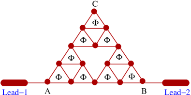
Figure 1: (Color online). A $3$-rd generation Sierpinski gasket is attached to two semi-infinite $1$D metallic leads, viz, lead-1 and lead-2. Each elementary plaquette of the gasket is penetrated by a magnetic flux $\phi$. The filled red circles correspond to the positions of the atomic sites.

practically any design can be tailor made, and the present work thus offers an excellent opportunity to study the simultaneous effects of magnetic field, electron-electron interaction and the dephasing caused by the introduction of a third lead in the system.

Our motivation behind the present work is two-fold. First, we observe that the multi-terminal transport in systems with multiply connected geometry is a very little addressed (or, unaddressed) problem. In particular, the in-built self similarity of systems such as the SPG opens up the possibility of investigating the tunneling or switching aspect of these systems at arbitrarily small scales of energy. Secondly, it is essential, for a completeness in the understanding of the spectral properties of fractal networks to know, if the well known multi-fractal, Cantor set energy spectrum of non-interacting electrons domany ; rammal ; banavar ; ghez ; schwalm1 ; andrade1 ; schwalm2 ; andrade2 ; schwalm3 still retains its character even in the presence of electron-electron interaction or dephasing caused by a third electrode. In a recent work, the effect of electron-electron interactions on the persistent current in a closed loop SPG has been reported sant2 , but no result exists for open self-similar systems connected to electron reservoirs by multiple leads.

On its own merit, the effect of electron-electron interaction on the spectral properties is of great importance. Several experiments done on fractal networks have studied the magnetoresistance, the

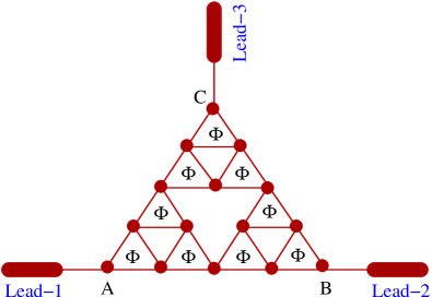
Figure 2: (Color online). A $3$-rd generation Sierpinski gasket is attached to three semi-infinite $1$D metallic leads, viz, lead-1, lead-2 and lead-3. Each elementary plaquette of the gasket is penetrated by a magnetic flux $\phi$. The filled red circles correspond to the positions of the atomic sites.

superconductor-normal phase boundaries on Sierpinski gasket wire networks gordon1 ; gordon2 ; gordon3 ; korshu ; meyer . These experiments pioneered the actual observational studies of spectral properties and flux quantization effects on planar networks and the Aharonov-Bohm effect in systems without translational invariance. Although in an early paper the problem of interacting electrons on a percolating cluster that displays a fractal geometry nedellec , has been addressed, to the best of our knowledge, no rigorous effort has been made so far to unravel the effect of an interplay of electron-electron interaction and an external magnetic field on deterministic networks such as a Sierpinski gasket (SPG), even at a mean field level.

Thus, apart from a critical investigation of the possibility of a fractal device, the present work is also likely to throw light on the fundamental spectral properties of the deterministically disordered systems.

We find quite interesting results. Working within a tight-binding framework we develop a mean field method of studying the three-terminal transport in interacting systems. The method is then applied to a planar SPG and we show that, dephasing definitely reduces the corner-to-corner propagation of electrons, with or without the electron-electron interaction. The magnetic field, in the absence of the electron-electron interaction generates an apparent continuum in the transmission spectrum. The continuum has already been observed in several fractal lattices arun2 ; arun3 ; schwalm4 including an SPG arun1 , and is practically unaffected even when the electron-electron interaction is switched ‘on’. A detailed study on the effect of positioning of the third electrode is also made, and the transport properties of an anisotropic gasket are compared with its isotropic counterpart. For a comparative study, the results of the two-terminal transport are also presented along with the three-terminal cases.

In what follows, we present our model quantum system in Section II. The essentials of the mean field calculation are discussed in Section III. Section IV contains the numerical results and related discussions, and we draw our conclusions in Section V.

II The model quantum systems

Let us begin by referring to Fig. 1 where a $3$-rd generation SPG is attached to two semi-infinite one-dimensional ($1$D) metallic leads, namely, lead-1 and lead-2 via the atomic sites A and B. Each elementary plaquette of the gasket is threaded by a magnetic flux $\phi$ (measured in unit of the elementary flux quantum $\phi_{0}=ch/e$). The filled red circles correspond to the positions of atomic sites in the SPG. In a Wannier basis the tight-binding Hamiltonian of the interacting gasket reads,

$$H_{\mbox{SPG}} = \sum_{i,\sigma}\epsilon_{i\sigma}c_{i\sigma}^{\dagger}c_{i\sigma}+\sum_{\langle ij\rangle,\sigma}v\left[e^{i\theta}c_{i\sigma}^{\dagger}c_{j\sigma}+h.c.\right]$$ (1)

$$+\sum_{i}Uc_{i\uparrow}^{\dagger}c_{i\uparrow}c_{i\downarrow}^{\dagger}c_{i\downarrow}$$

where, $\epsilon_{i\sigma}$ is the on-site energy of an electron at the site $i$ of spin $\sigma$ ($\uparrow,\downarrow$) and $v$ is the nearest-neighbor hopping strength. In the case of an anisotropic SPG, the anisotropy is introduced only in the nearest-neighbor hopping integral $v$ which takes on values $v_{x}$ and $v_{y}$ for hopping along the horizontal and the angular bonds, respectively. Due to the presence of magnetic flux $\phi$, a phase factor $\theta=2\pi\phi/3$ appears in the Hamiltonian when an electron hops from one site to another site. A negative sign comes in when the electron hops in the reverse direction. As the magnetic filed associated with $\phi$ does not penetrate any part of the circumference of the elementary triangle, we ignore the Zeeman term in the above tight-binding Hamiltonian (Eq. 1). $c_{i\sigma}^{\dagger}$ and $c_{i\sigma}$ are the creation and annihilation operators, respectively, of an electron at the site $i$ with spin $\sigma$. $U$ is the strength of on-site Coulomb interaction. The Hamiltonian for the non-interacting leads can be expressed as,

$$H_{\mbox{lead}}=\sum_{i}\epsilon_{0}c_{i}^{\dagger}c_{i}+\sum_{<ij>}t_{0}\left(c_{i}^{\dagger}c_{j}+c_{j}^{\dagger}c_{i}\right)$$ (2)

where different parameters correspond to their usual meaning. These leads are directly coupled to the gasket where the hopping integral between the lead-1 and gasket is $\tau_{1}$, and, it is $\tau_{2}$ between the gasket and lead-2. With this setup we investigate two-terminal electron transport through an SPG.

For three-terminal quantum transport we connect an additional lead with the gasket. A schematic view of a $3$-rd generation SPG attached to three semi-infinite $1$D metallic leads, viz, lead-1, lead-2 and lead-3 is shown in Fig. 2. The gasket and the side-attached leads are described by the same prescriptions as described above.

III The mean field approach

III.1 Decoupling of the interacting Hamiltonian

Before going to the calculation of electronic transmission probability through the interacting model of an SPG described by the tight-binding Hamiltonian given in Eq. 1, first we decouple the interacting Hamiltonian using the generalized Hartree-Fock approach kato ; kam ; sant5 . The full Hamiltonian is completely decoupled into two parts. One is associated with the up-spin electrons, while the other is with the down-spin electrons. The on-site potentials get modified appropriately, and are given by,

$$\epsilon_{i\uparrow}^{\prime}=\epsilon_{i\uparrow}+U\langle n_{i\downarrow}\rangle$$ (3)

$$\epsilon_{i\downarrow}^{\prime}=\epsilon_{i\downarrow}+U\langle n_{i\uparrow}\rangle$$ (4)

where, $n_{i\sigma}=c_{i\sigma}^{\dagger}c_{i\sigma}$ is the number operator. With these site energies, the full Hamiltonian (Eq. 1) can be written in the decoupled form (in the mean field (MF) approximation) as,

$$H_{\mbox{MF}} = \sum_{i}\epsilon_{i\uparrow}^{\prime}n_{i\uparrow}+\sum_{\langle ij\rangle}v\left[e^{i\theta}c_{i\uparrow}^{\dagger}c_{j\uparrow}+e^{-i\theta}c_{j\uparrow}^{\dagger}c_{i\uparrow}\right]$$ (5)

$$+ \sum_{i}\epsilon_{i\downarrow}^{\prime}n_{i\downarrow}+\sum_{\langle ij\rangle}v\left[e^{i\theta}c_{i\downarrow}^{\dagger}c_{j\downarrow}+e^{-i\theta}c_{j\downarrow}^{\dagger}c_{i\downarrow}\right]$$

$$- \sum_{i}U\langle n_{i\uparrow}\rangle\langle n_{i\downarrow}\rangle$$

$$= H_{\mbox{SPG},\uparrow}+H_{\mbox{SPG},\downarrow}-\sum_{i}U\langle n_{i\uparrow}\rangle\langle n_{i\downarrow}\rangle$$

where, $H_{\mbox{SPG},\uparrow}$ and $H_{\mbox{SPG},\downarrow}$ correspond to the effective tight-binding Hamiltonians for the up and down spin electrons, respectively. The last term is a constant term which provides a shift in the total energy.

III.2 Self consistent procedure

With these decoupled Hamiltonians ($H_{\mbox{SPG},\uparrow}$ and $H_{\mbox{SPG},\downarrow}$) of up and down spin electrons, now we start our self consistent procedure considering initial guess values of $\langle n_{i\uparrow}\rangle$ and $\langle n_{i\downarrow}\rangle$. For these initial set of values of $\langle n_{i\uparrow}\rangle$ and $\langle n_{i\downarrow}\rangle$, we numerically diagonalize the up and down spin Hamiltonians. Then we calculate a new set of values of $\langle n_{i\uparrow}\rangle$ and $\langle n_{i\downarrow}\rangle$. These steps are repeated until a self consistent solution is achieved.

III.3 Two-terminal quantum system

Now we are at the stage of calculating electron conduction across an SPG.

To determine two-terminal conductance ($g$) of the gasket, we use Landauer conductance formula datta . At much low temperature and bias voltage it can be expressed as,

$$g=\frac{e^{2}}{h}\left(T_{\uparrow}+T_{\downarrow}\right)$$ (6)

where, $T_{\uparrow}$ and $T_{\downarrow}$ correspond to the transmission probabilities of up and down spin electrons, respectively, across the SPG. Since no spin-flip scattering term exists in the Hamiltonian (Eq. 1), spin-flip transmission probabilities will not appear in Eq. 6. In terms of the Green’s function of the gasket and its coupling to side-attached leads, transmission probability can be written in the form datta ,

$$T_{\sigma}={\mbox{Tr}}\left[\Gamma_{1}\,G_{\mbox{SPG},\sigma}^{r}\,\Gamma_{2}\,G_{\mbox{SPG},\sigma}^{a}\right]$$ (7)

where, $\Gamma_{1}$ and $\Gamma_{2}$ describe the coupling of the SPG to the lead-$1$ and lead-$2$, respectively. Here, $G_{\mbox{SPG},\sigma}^{r}$ and $G_{\mbox{SPG},\sigma}^{a}$ are the retarded and advanced Green’s functions, respectively, of the SPG including the effects of the leads. Now, for the complete system i.e., the SPG and two leads, the Green’s function is expressed as,

$$G_{\sigma}=\left(E-H_{\sigma}\right)^{-1}$$ (8)

where, $E$ is the energy of the injecting electron. Evaluation of this Green’s function needs the inversion of an infinite matrix, which is really a difficult task, since the full system consists of the finite size gasket and two semi-infinite $1$D leads. However, the full system can be partitioned into sub-matrices corresponding to the individual sub-systems and the Green’s function for the gasket can be effectively written as,

$$G_{\mbox{SPG},\sigma}=\left(E-H_{\mbox{SPG},\sigma}-\Sigma_{1}-\Sigma_{2}\right)^{-1}$$ (9)

where, $\Sigma_{1}$ and $\Sigma_{2}$ are the self-energies due to coupling of the gasket to the lead-$1$ and lead-$2$, respectively. All information of the coupling are included into these self-energies.

III.4 Three-terminal quantum system

In order to calculate the conductance in three-terminal SPG, we use Büttiker formalism, an elegant and simple way to study electron transport through multi-terminal mesoscopic systems. In this formalism we treat all the leads (current and voltage leads) on an equal footing and extend the two-terminal linear response formula to get the conductance between the terminals, indexed by $p$ and $q$, in the form datta ; buttiker2 ,

$$g_{pq}=\frac{e^{2}}{h}\left(T_{pq,\uparrow}+T_{pq,\downarrow}\right)$$ (10)

where, $T_{pq,\sigma}$ gives the transmission probability of an electron with spin $\sigma$ ($\uparrow,\downarrow$) from the lead-$p$ to lead-$q$.

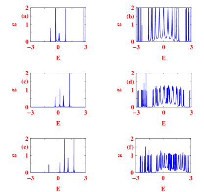
Figure 3: (Color online). Two-terminal conductance $g$ as a function of energy $E$ for a $4$-th generation isotropic ($v_{x}=v_{y}=1$) Sierpinski gasket ($N=42$), where lead-1 and lead-2 are connected at the positions A and B, respectively. The first and second columns correspond to $\phi=0$ and $0.25$, respectively, where the upper, middle and lower panels represent $U=0$, $1$ and $2$, respectively.

Now, similar to Eq. 7 the transmission probability $T_{pq,\sigma}$ can be expressed in terms of the SPG-lead coupling matrices and the effective Green’s function of the SPG as datta ,

$$T_{pq,\sigma}={\mbox{Tr}}\left[\Gamma_{p}\,G_{\mbox{SPG},\sigma}^{r}\,\Gamma_{q}\,G_{\mbox{SPG},\sigma}^{a}\right].$$ (11)

In the presence of multi-leads, the effective Green’s function of the SPG becomes (extension of Eq. 9) datta ,

$$G_{\mbox{SPG},\sigma}=\left(E-H_{\mbox{SPG},\sigma}-\sum_{p}\Sigma_{p}\right)^{-1}$$ (12)

where, $\Sigma_{p}$ is the self-energy due to coupling of the SPG to the lead-$p$ and the sum over $p$ runs from $1$ to $3$.

In the present work we inspect all the essential features of magnetic response of an SPG network at absolute zero temperature and use the units where $c=h=e=1$. Throughout our numerical work we set $\epsilon_{i\uparrow}=\epsilon_{i\downarrow}=0$ for all $i$ and choose the nearest-neighbor hopping strength $v=1$. In the anisotropic case we select $v_{x}=1$ and $v_{y}=2$ throughout. For side-attached leads,

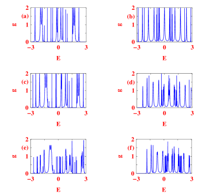
Figure 4: (Color online). Two-terminal conductance $g$ as a function of energy $E$ for a $4$-th generation anisotropic ($v_{x}=1$ and $v_{y}=2$) Sierpinski gasket ($N=42$), where lead-1 and lead-2 are connected at the positions A and B, respectively. The first and second columns correspond to $\phi=0$ and $0.25$, respectively, where the upper, middle and lower panels represent $U=0$, $1$ and $2$, respectively.

the on-site energy ($\epsilon_{0}$) and nearest-neighbor hopping strength ($t_{0}$) are fixed at $0$ and $1.5$, respectively. The hopping integrals ($\tau_{1}$, $\tau_{2}$ and $\tau_{3}$) between the leads and SPG are set at $0.5$. Energy scale is measured in unit of $v$. All the essential features of electron transport are obtained both for an isotropic gasket and its anisotropic counterpart.

IV Numerical results and discussion

IV.1 Two-terminal quantum transport

The two-terminal conductance of a $4$-th generation isotropic gasket is shown in Fig. 3 with the leads connected in the positions A and B only. The left panel shows the conductance in zero magnetic field, and represents the familiar fragmented, scanty distribution of the transmission resonances that mark such a lattice. The on-site Hubbard interaction displaces the resonance peaks, but no marked changes in the spectrum is observed.

With the magnetic field turned ‘on’ there is however, a remarkable change. The spectrum apparently exhibits continuous parts, which have previously been reported arun1 to support extended single particle states for spinless, non-interacting electrons. We observe here that, the electron-electron interaction, though reduces the overall conductance of the system, preserves the continuum at the central part of the spectrum. As the interaction $U$ is increased, the central continuum is more or less undisturbed, though the average transmission amplitude still exhibits lower values compared to its $U=0$ counterpart. In addition, there is a signature of opening up of new gaps in the spectrum as it appears in Fig. 3(f).

In Fig. 4 we show the two-terminal conductance across an SPG of the same size as before, but now with a hopping anisotropy such that, $v_{x}=1$ and $v_{y}=2$. The effect of hopping anisotropy is, in general, to

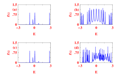
Figure 5: (Color online). Three-terminal conductance $g_{12}$ as a function of energy $E$ for a $4$-th generation isotropic ($v_{x}=v_{y}=1$) Sierpinski gasket ($N=42$), where lead-1, lead-2 and lead-3 are connected at the positions A, B and C, respectively. For this arrangement of side attached leads (symmetric configuration), all $g_{ij}$’s ($i\neq j$) are identical to each other. (a) $U=0$, $\phi=0$; (b) $U=0$, $\phi=0.25$; (c) $U=2$, $\phi=0$ and (d) $U=2$, $\phi=0.25$.

increase the overall conductance. The sparse spectrum in the left panel of Fig. 3 is now replaced by a substantial density of resonant transmission peaks. The introduction of $U$ still reduces the average conductance, but the action is now somewhat ‘delayed’. We need a larger value of $U$ to generate a noticeable change in the conductance spectrum. This is evident from the left panel of Fig. 4. On the right panel, the interplay of the magnetic field and the electron-electron interaction is displayed. The central continuum of the isotropic gasket case is still there, but with numerous conductance minima somewhat obscuring the continuity of this part. As $U$ increases, one observes genuine anti-resonances in the previously sustained continuum in the spectrum.

IV.2 Three-terminal quantum transport

We now discuss the three-terminal transport in a SPG network. On the left panel of Fig. 5 the results of the conductance between the leads $1$ and $2$ are shown. The third terminal $3$ connects to

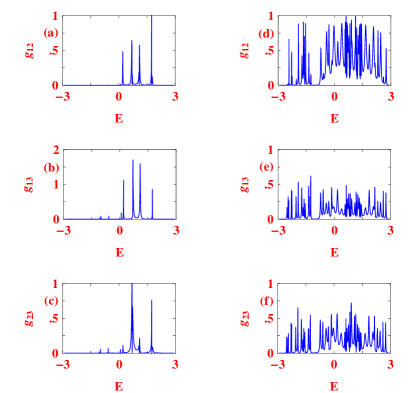
Figure 6: (Color online). Three-terminal conductance $g_{ij}$ as a function of energy $E$ for a $4$-th generation isotropic ($v_{x}=v_{y}=1$) Sierpinski gasket ($N=42$), where lead-1 and lead-2 are connected at the positions A and B, respectively. Lead-3 is attached at the centre of the line BC. This is the so-called asymmetric configuration of the leads. First column corresponds to $\phi=0$, while the second column represents $\phi=0.25$. For all these spectra we set $U=2$.

an electron reservoir. The effect of dephasing is obvious. The spectrum in zero magnetic field is even thinner now, and the interaction $U$ plays its part. The magnitude of the resonance peaks get suppressed compared to the coherent transport in the two-terminal case. A fine scrutiny (not shown here) will reveal a level broadening due a dominant phase randomizing effect sant3 leading to a loss of phase coherence. Strangely enough, in presence of the magnetic field, the dephasing effect is just not enough to destroy or alter appreciably, the central continuous part of the conductance spectrum. We have carried out extensive numerical analysis of the continuum in the conductance spectrum, and it appears that the band remains intact over finer scales of energy interval and even for a larger sized SPG. Therefore, we are tempted to conclude that there exists a band of extended eigenstates (characterized by finite transmittivity) in an SPG fractal threaded by a magnetic field perpendicular to the plane of the gasket and that, its a quite robust band, unperturbed by either the electron-electron interaction, or the presence of any dephasing effect.

In the asymmetric case however, the conductance is strongly sensitive on the lead positions. For example, with $v_{x}=1$ and $v_{y}=2$, the conductance $g_{12}$ across the $1$-$2$ terminals is much larger compared to $g_{23}$ or $g_{13}$, particularly in presence of the magnetic field. The apparent continuum in the spectrum persists, as before, even with an increasing value of $U$. The results are displayed in Fig. 6.

V Conclusion

In conclusion, we have examined in details, the three-terminal transport in a planar Sierpinski gasket fractal with a magnetic field threading each elementary triangle. The electron-electron interaction is considered in the Hubbard form, and the Hamiltonian is solved within a generalized Hartree-Fock scheme. The sensitivity of the conductance spectrum on the positioning of the leads is studied extensively, and some prototype results have been displayed and discussed. It is seen that the major role of the third lead is to bring down the average conductance of the system. The same role is played by the Hubbard interaction. The anisotropic gasket has been found to be more conducting than its isotropic counterpart with or without the electron-electron interaction. However, the curious result is that, the continuum of states generated in the spectrum of an SPG as the magnetic field is turned on, is practically unaffected by the dephasing effect caused by the additional electrode or by the on-site Hubbard interaction.

References

- (1) A. Aviram and M. A. Ratner, Chem. Phys. Lett. 29, 277 (1974).
- (2) C. Joachim, J. K. Gimzewski, and A. Aviram, Nature 408, 541 (2000).
- (3) M. A. Reed, C. Zhou, C. J. Muller, T. P. burgin, and J. M. Tour, Science 278, 252 (1997).
- (4) T. Sekitani, U. Zschieschang, H. Klauk, and T. Someya, Nat. Mater. 9, 1015 (20100.
- (5) R. de Picciotto, H. L. Stormer, L. N. Pfeiffer, K. W. Baldwin, and K. W. West, Nature 411, 51 (2001).
- (6) M. Sigrist, A. Fuhrer, T. Ihn, K. Ensslin, S. Ulloa, W. Wegescheider, and M. Bichler, Phys. Rev. Lett. 93, 066802 (2004).
- (7) H. Song, Y. Kim, Y. H. Jang, H. Jeong, M. A. Reed, and T. Lee, Nature 462, 1039 (2009).
- (8) O. Entin-Wohlman, A. Aharony, Y. Imry, Y. Levinson, and A. Schiller, Phys. Rev. Lett. 88, 166801 (2002).
- (9) A. Aharony, O. Entin-Wohlman, B. I. Halperin, and Y. Imry, Phys. Rev. B 66, 115311 (2002).
- (10) Y. S. Joe, E. R. Hadin, and A. M. Satanin, Phys. Rev. B 76, 085419 (2007).
- (11) T. Jayasekara and J. W. Mintmire, Nanotechnology 18, 424033 (2007).
- (12) C. Ritter, M. Pacheco, P. Orellana, and A. Latge, J. Appl. Phys. 106, 104303 (2009).
- (13) K. K. Saha, W. Lee, J. bernholc, and V. Meunier, J. Chem. Phys. 131, 164105 (2009).
- (14) H. U. Baranger, D. P. Di Vincenzo, R. A. Jalabert, and A. D. Stone, Phys. Rev. B 44, 10637 (1991).
- (15) M. Büttiker, Phys. Rev. Lett. 57, 1761 (1986).
- (16) S. K. Maiti, Solid State Commun. 150, 1269 (2010).
- (17) B. G. Cook, P. Dignard, and K. Varga, Phys. Rev. B 83, 205105 (2011).
- (18) D. M. Cardamone, C. A. Stafford, and S. Majumdar, Nano Lett. 6, 2422 (2006).
- (19) P. Dutta, S. K. Maiti, and S. N. Karmakar, Org. Electron. 11, 1120 (2010).
- (20) S. Datta, Electronic transport in mesoscopic systems, Cambridge University Press, Cambridge (1997).
- (21) S. V. Faleev, F. Léonard, D. A. Stewart, and M. van Schilfgaarde, Phys. Rev. B 71, 195422 (2005).
- (22) J. J. Palacios, A. J. Pérez-Jiménez, E. Louis, E. SanFabián, and J. A. Vergés, Phys. Rev. Lett. 90, 106801 (2003).
- (23) Y. Xue, S. Datta, and M. Ratner, J. Chem. Phys. 115, 4292 (2001).
- (24) S. Sanvito, C. J. Lambert, J. H. Jefferson, and A. M. Bratkovsky, Phys. Rev. B 59, 11936 (1999).
- (25) L. Onsager, Phys. Rev. 38, 2265 (1931).
- (26) M. Büttiker, Phys. Rev. B 33, 3020 (1986).
- (27) M. Büttiker, IBM J. Res. Dev. 32, 63 (1988).
- (28) E. Domany, S. Alexander, D. Bensimon, and L. P. Kadanoff, Phys. Rev. 28, 3110 (1982).
- (29) R. Rammal and G. Toulose, Phys. Rev. Lett. 49, 1194 (1982).
- (30) J. R. Banavar, L. Kadanoff, and A. M. M. Pruisken, Phys. Rev. B 31, 1388 (1984).
- (31) J. M. Ghez, Y. Y. Wang, R. Rammal. B. Pannetier, and J. B. Bellisard, Solid State Commun. 64, 1291 (1987).
- (32) W. A. Schwalm and M. K. Schwalm, Phys. Rev. B 39, 12872 (1989).
- (33) R. F. S. Andrade H. J. Schellnhuber, Europhys. Lett. 10, 73 (1989).
- (34) W. A. Schwalm and M. K. Schwalm, Phys. Rev. B 44, 382 (1991).
- (35) R. F. S. Andrade and H. J Schellnhuber, Phys. Rev. B 44, 13213 (1991).
- (36) W. A. Schwalm and M. K. Schwalm, Phys. Rev. B 47, 7847 (1993).
- (37) B. Kubala and J. König, Phys. Rev. B 67, 205303 (2003); Phys. Rev. B 65, 245301 (2002).
- (38) B. Kubala and J. König, Phys. Rev. B 65, 245301 (2002).
- (39) S. K. Maiti and A. Chakrabarti, Phys. Rev. B 82, 184201 (2010).
- (40) J. M. Gordon, A. M. goldman, J. Maps, D. Costello, R. Tiberio, and B. Whitehead, Phys. Rev. Lett. 56, 2280 (1986).
- (41) J. M. Gordon, A. M. Goldman, and B. Whitehead, Phys. Rev. Lett. 59, 2311 (1987).
- (42) J. M. Gordon and A. M. Goldman, Phys. Rev. B 35, 4909 (1987).
- (43) S. E. Korshunov, R. Meyer, and P. Martinoli, Phys. Rev. B 51, 5914 (1995).
- (44) R. Meyer, S. E. Korshunov, Ch. Leemann, and P. Martinoli, Phys. Rev. B 66, 104503 (2002).
- (45) P. Nedellec, M. Aprili, J. Lesueur, and L. Dumoulin, Solid State Commun. 102, 41 (1993).
- (46) A. Chakrabarti, Phys. Rev. B 60, 10576 (1999).
- (47) A. Chakrabarti, Phys. Rev. B 72, 134207 (2005).
- (48) W. Schwalm and B. J. Moritz, Phys. Rev. B 71, 134207 (2005).
- (49) A. Chakrabarti and B. Bhattacharyya, Phys. Rev. B 56, 13768 (1997).
- (50) H. Kato and D. Yoshioka, Phys. Rev. B 50, 4943 (1994).
- (51) A. Kambili, C. J. Lambert, and J. H. Jefferson, Phys. Rev. B 60, 7684 (1999).
- (52) S. K. Maiti, Solid State Commun. 150, 2212 (2010).
- (53) M. Dey, S. K. Maiti, and S. N. Karmakar, Org. Electron. 12, 1017 (2011).