Identical temperature dependence of the time scales of several linear-response functions of two glass-forming liquids

Abstract

The frequency-dependent dielectric constant, shear and adiabatic bulk moduli, longitudinal thermal expansion coefficient, and longitudinal specific heat have been measured for two van der Waals glass-forming liquids, tetramethyl-tetraphenyl-trisiloxane (DC704) and 5-polyphenyl-4-ether. Within the experimental uncertainties the loss-peak frequencies of the measured response functions have identical temperature dependence over a range of temperatures, for which the Maxwell relaxation time varies more than nine orders of magnitude. The time scales are ordered from fastest to slowest as follows: Shear modulus, adiabatic bulk modulus, dielectric constant, longitudinal thermal expansion coefficient, longitudinal specific heat. The ordering is discussed in light of the recent conjecture that van der Waals liquids are strongly correlating, i.e., approximate single-parameter liquids.

A liquid has several characteristic times Boon1980 ; Brawer1985 ; March2002 ; Barrat2003 . One is the Maxwell relaxation time determining how fast stress relaxes $\tau_{\text{M}}\equiv\eta/G_{\infty}$, where $\eta$ is the shear viscosity and $G_{\infty}$ the instantaneous shear modulus Harrison1976 . Other characteristic times are identified by writing $D=a^{2}/\tau_{D}$, in which $D$ may be particle, heat, or the transverse momentum diffusion constant, and $a$ is of order the intermolecular distance. Further characteristic times are the inverse loss-peak frequencies (i.e., frequencies of maximum imaginary part) of different complex frequency-dependent linear-response function Angell2000 ; Kremer2002 . For low-viscosity liquids like ambient water the characteristic times are all of the same order of magnitude, in the picosecond range, and only weakly dependent on temperature.

Supercooling a liquid increases dramatically its viscosity Angell1995 ; Debenedetti1996 ; Donth2001 ; Binder2005 ; Dyre2006a ; most characteristic times likewise increase dramatically. The metastable equilibrium liquid can be cooled until the relaxation times become $10^{10}$–$10^{15}$ times larger than for the low-viscosity liquid, at which point the system falls out of metastable equilibrium and forms a glass. At typical laboratory cooling rates ($\text{K}/\text{min}$) the glass transition takes place when $\tau_{\text{M}}$ is of order 100 seconds Angell1995 ; Debenedetti1996 ; Donth2001 ; Binder2005 ; Dyre2006a .

Even though most characteristic times increase dramatically when the liquid is cooled, they are generally not identical. Different measured quantities and different definitions of the characteristic time scale lead to somewhat different characteristic times. A trivial example is the difference between the time scales of the bulk modulus and its inverse in the frequency domain, the bulk compressibility. More interestingly, some time scales might have quite different temperature dependence; this is often referred to as a decoupling of the corresponding microscopic processes.

Several relaxation time decouplings have been reported in the ultraviscous liquid state above the glass transition. Significant decoupling takes place for some glass-forming molten salts like “CKN” (a 60/40 mixture of ${\rm Ca(NO_{3})_{2}}$ and ${\rm KNO_{3}}$ Angell1964 ), where the conductivity relaxation time at the glass transition is roughly $10^{4}-10^{5}$ times smaller than $\tau_{\text{M}}$ Angell1988 ; Angell1991 . This reflects a decoupling of the molecular motions, with the cations diffusing much faster than the nitrate ions Angell1991 . A more recent discovery is the decoupling of translational and rotational motion in most molecular liquids, for which one often finds that molecular rotations are 10-100 times slower than expected from the diffusion time Fujara1992 ; Cicerone1996 ; Sillescu1999 . This is generally believed to reflect dynamic heterogeneity of glass-forming liquids Fujara1992 ; Cicerone1996 ; Sillescu1999 ; Ediger2000 . Angell in 1991 suggested a scenario consisting of “a series of decouplings which occurs on decreasing temperature”, sort of a hierarchy. He cautiously added, though, that “more data are urgently needed to decide if this represents the general case” Angell1991 .

Some linear-response functions like the thermoviscoelastic and shear-mechanical ones are difficult to measure reliably for ultraviscous liquids Christensen1995 ; Christensen2007 ; Christensen2008 . To the best of our knowledge there are no studies of their possible decoupling. This paper presents such data, together with conventional dielectric data. The purpose is to establish the order of relaxation times among the different quantities and, in particular, to investigate whether or not they show a decoupling upon approaching the glass-transition temperature.

I Experimental results

We have measured the complex, frequency-dependent dielectric constant $\varepsilon(\omega)$, shear modulus $G(\omega)$ Christensen1995 ; HecksherPHD , adiabatic bulk modulus $K_{S}(\omega)$ Christensen1994b ; HecksherPHD , and longitudinal specific heat $c_{l}(\omega)$ Jakobsen2010 on two van der Waals bonded glass-forming liquids tetramethyl-tetraphenyl-trisiloxane (DC704) and 5-polyphenyl-4-ether (5PPE) (commercial vacuum-pump oils). For DC704 the time-dependent longitudinal thermal expansion coefficient $\alpha_{l}(t)$ NissAlpha was also measured (see appendix B for details). We note that both liquids have linear-response functions that to a good approximation obey time-temperature superposition (TTS) Olsen2001 ; Jakobsen2005 ; HecksherPHD , i.e., their loss-peak shapes are temperature independent in log-log plots. Moreover, the two liquids have only small beta relaxations, they rarely crystallize, and they are generally very stable and reproducible — altogether these two liquids are very suitable for fundamental studies.

Three of the measured quantities ($\alpha_{l}$, $c_{l}$, and $K_{S}$) are closely related to one complete set of independent scalar thermoviscoelastic response functions : $c_{p}$, $\alpha_{p}$, and $\kappa_{T}$ (the relations are given in appendix C). Measurements of such a complete set of three scalar thermoviscoelastic response functions are rare, if at all existing for any glass-forming liquid.

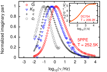
Figure 1: Example of data from which loss-peak positions are found. Main part: Normalized imaginary parts of the following complex response functions: shear modulus $G(\omega)$, adiabatic bulk modulus $K_{S}(\omega)$, dielectric constant $\epsilon(\omega)$, and longitudinal specific heat $c_{l}(\omega)$, as functions of frequency for 5-polyphenyl-4-ether (5PPE) at $T=252.5$. Inset: Time-dependent longitudinal expansion coefficient $\alpha_{l}(t)$ at $T=209.2$ for tetramethyl-tetraphenyl-trisiloxane (DC704).

Figure 1 shows the normalized loss peaks as functions of frequency of $G(\omega)$, $K_{S}(\omega)$, $\epsilon(\omega)$, and $c_{l}(\omega)$ for 5PPE at $252.5$. The inset shows one data set for the time-dependent $\alpha_{l}(t)$ at $T=209.2$ for DC704. The frequency-domain data allow for direct determination of the loss-peak frequencies ($\nu_{\text{lp}}$); the time-domain data were Laplace transformed to give an equivalent loss-peak frequency NissAlpha .

The measurements give both real and imaginary parts of the complex response functions, allowing us to calculate two other relevant characteristic frequencies, namely the inverse Maxwell time $1/(2\pi\tau_{\text{M}})$ ($\eta$ and $G_{\infty}$ can be found from $G(\omega)$) and the loss-peak frequency of the adiabatic compressibility $\kappa_{S}(\omega)=1/K_{S}(\omega)$. Figure 2(a) shows the temperature dependence of the seven characteristic frequencies for DC704online . The data cover more than nine decades in relaxation time (from $T_{g}$ and up). Clearly the time scales for the response functions follow each other closely.

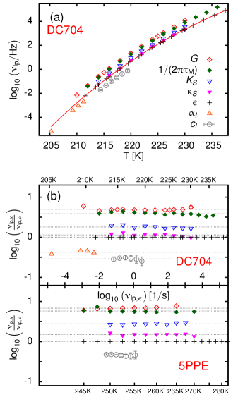
Figure 2: (a) Seven characteristic frequencies (based on five measured quantities) as functions of temperature for DC704. The full curve is a fit of the dielectric data to a Parabolic functionGarrahan2003 ; *Elmatad2009; *Elmatad2010 (see appendix D for details on this function), used for extrapolation of the dielectric data to low temperatures. Filled symbols ($\tau_{\text{M}}$ and $\kappa_{S}$) indicate that the quantity in question is not measured directly, but derived from one of the measured quantities. Error bars on $c_{l}$ data were estimated by assuming an additive influence from the underlying spurious frequency dependence of the raw data Jakobsen2010 , varying its influence on the loss peak from negligible to maximal. Equivalent data are given for 5PPE in appendix A.
(b) Time-scale index of all measured response functions (symbols as in the top figure) with respect to the dielectric constant for the two liquids DC704 and 5PPE. The time-scale index is plotted as functions of the dielectric loss-peak frequency (common X-axis), which represents the temperature (also given for each liquid). For both liquids the time-scale index for all quantities are temperature independent within the experimental uncertainty, that is, the measured quantities have the same temperature dependence of their characteristic time scales.

Figure 2(b) plots the characteristic frequencies in terms of a “time-scale index” defined as the logarithmic distance to the dielectric loss-peak frequency. For both liquids the time-scale indices are temperature independent within the experimental uncertainty, that is, the characteristic time scales of the measured quantities change in the same way with temperature.

This finding constitutes the main result of the present paper, showing that the time scales for theses response functions are strongly coupled, in contrast to the observed decoupling between transitional diffusion and rotationFujara1992 ; Cicerone1996 ; Sillescu1999 and at variance with the scenario suggested by AngellAngell1991 .

II Discussion

The fastest response function is the shear modulus. It has previously been reported that this quantity is faster than dielectric relaxation for a number of glass-forming liquids (see e.g. Ref. Deegan1999, and Ref. Jakobsen2005, and references therein), a fact that the Gemant-DiMarzio-Bishop model explains qualitatively Niss2005 . The dielectric relaxation is faster than the specific heat (this difference cannot be attributed to measuring $c_{l}$ and not $c_{p}$ supmat ). For glycerol the same tendency has been reported Ngai1990 ; Schroter2000 , but with a fairly small difference in time scales of $c_{p}$ and $\epsilon$ ($\approx 0.2$ decades). However a consistent interpretation of dielectric hole-burning experiments on glycerol was arrived at by assuming that these two time scales coincide Weinstein2005 . For propylene glycol the opposite trend has been reported Ngai1990 . Regarding volume and enthalpy relaxation there is likewise no general trend in the literature; some glass-formers have slower enthalpy than volume relaxation, others the opposite Sasabe1978 ; Adachi1982 ; Badrinarayanan2007 . Clearly more work is needed to identify any possible general trends. However, such comparisons are difficult, as it requires a precision in absolute temperature at least better than $1$ between the experiments. This is very difficult to obtain, and it could be speculated that some of the contradicting results could be explained this way. An advantage of our methods is that the same cryostat can be used for all the measurements ensuring same absolute temperature (see appendix B).

What does theory have to say about the decoupling among relaxation functions and why some are faster than others? As mentioned, there are three independent scalar thermoviscoelastic response functions. There is no a priori reason these should have even comparable loss-peak frequencies. Moreover, both the dielectric constant and the shear modulus are linear-response functions that do not belong to the class of scalar thermoviscoelastic response functions; these two functions could in principle have relaxation times entirely unrelated to those of the scalar thermoviscoelastic response functions. All in all, general theory does not explain our findings.

As mentioned earlier, the two investigated liquids obey TTS to a good approximation and have very small (if existing) beta relaxations. In an earlier work (Ref. Jakobsen2005, ) some of us noticed that the time-scale index between shear mechanical and dielectric relaxation is only significantly temperature dependent for systems with a significant beta relaxation. In Ref. Hecksher2010, it was shown for a number of systems (including systems with a pronounced beta relaxation) that the dielectric relaxation and the aging rate after a temperature jump follow the same “inner clock”; these results were obtained at temperatures where the alpha and beta relaxations are well separated. Based on this, one might speculate that some (or all) of the temperature dependencies of the time-scale index observed in the literature could be due to the difference in the influence from the beta relaxation between the measured response functions (see e.g. Ref. Jakobsen2011, for a comparison of the influence in shear mechanical and dielectric relaxation).

II.1 Comparison to a “perfectly correlating liquid”

The class of so-called “strongly correlating” liquids was recently identified Pedersen2008 ; *Bailey2008; *Bailey2008a; *Schroder2009a; *Gnan2009; *Schroder2009; *Pedersen2010; *Gnan2010. This class includes most or all van der Waals and metallic liquids, but not the covalently-bonded, hydrogen-bonded, or ionic liquids. In computer simulations strongly correlating liquids are characterized by strong correlations between constant-volume equilibrium fluctuations of virial and potential energy Pedersen2008 ; *Bailey2008; *Bailey2008a; *Schroder2009a; *Gnan2009; *Schroder2009; *Pedersen2010; *Gnan2010. These liquids are approximate single-parameter liquids, i.e., they do not have three independent isotropic scalar thermoviscoelastic response functions, but to a good approximation merely one Bailey2008b . A perfect single-parameter liquid obeysEllegaard2007

$$\frac{T_{0}\alpha_{p}^{\prime\prime}(\omega)}{c_{p}^{\prime\prime}(\omega)}=\gamma_{Tp}=\frac{\kappa_{T}^{\prime\prime}(\omega)}{\alpha_{p}^{\prime\prime}(\omega)}$$ (1)

where $\gamma_{Tp}$ is a constant. Experimental evidence that DC704 is a strongly correlating liquid, was very recently presented in Ref. Gundermann2011, .

We tested how well our results conform to the predictions for a perfectly correlating liquid. If the thermoviscoelastic response functions obey Eq. (1), the loss-peak frequencies should be identical at all temperatures. A single-parameter model liquid was constructed by assuming Eq. (1) to hold, with high-frequency limits and relaxation strengths of the quantities chosen to be as close as possible to those measured for DC704. The quantities $\alpha_{l}(\omega)$, $c_{l}(\omega)$, and $\kappa_{S}(\omega)$ were calculated in the model by introducing shear-modulus data (see appendix C for details).

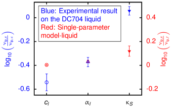
Figure 3: Time-scale indices of $c_{l}$, $\alpha_{l}$, and $\kappa_{S}$ for DC704 (blue symbols, left y-axis) and for the single-parameter model-liquid (red symbols, right y-axis) (see appendix C for details on the model calculation). The two axis have been shifted with respect to each other to give an overall best overlap of the indices. For the experimental data the time-scale index is given relative to the dielectric loss-peak frequency ($\nu_{\text{lp},\epsilon}$). The reported quantity is the mean over the index in Fig. 2(b), the error is based on the standard deviation (in the case of $c_{l}$ a mean over maximum and minimum based on the error bars on the loss-peak frequency was used). For the single-parameter model-liquid the index is with respect to the common loss-peak frequency of $\alpha_{p}$, $c_{p}$, and $\kappa_{T}$ ($\nu_{\text{lp},f}$). The model liquid has the same order of the time scales as the real liquid, but the differences in the time scales are underestimated in the model.

Figure 3 compares the characteristic frequencies of $c_{l}$, $\alpha_{l}$, and $\kappa_{S}$ of our experiments to those of the model liquid. The order of the time scales for the model liquid matches the observations, i.e., $c_{l}$ slower that $\alpha_{l}$ and $\kappa_{S}$ faster than $\alpha_{l}$. However, the magnitude of the time-scale differences is significantly underestimated.

III Summary

We measured several complex frequency-dependent linear-response functions on the two van der Waals liquids DC704 and 5PPE. Within the experimental uncertainties the time scales of the response functions have the same temperature dependence, that is, the time-scale indices are temperature independent. The time scales are for both liquids ordered from fastest to slowest as follows: Shear modulus, adiabatic bulk modulus, dielectric constant, longitudinal thermal expansion coefficient, longitudinal specific heat.

General theory does not explain why the time scales from some response functions couple very closely to each other, as is the case for the investigated response functions, and why others show a decoupling, as is observed, e.g. between transitional diffusion and rotationFujara1992 ; Cicerone1996 ; Sillescu1999 . The ordering of the longitudinal thermal expansion coefficient, the longitudinal specific heat and the adiabatic compressibility can be rationalized by assuming that the liquids are strongly correlating, i.e., approximate single-parameter liquidsPedersen2008 ; *Bailey2008; *Bailey2008a; *Schroder2009a; *Gnan2009; *Schroder2009; *Pedersen2010; *Gnan2010; Ellegaard2007 , in which certain sets of isotropic scalar thermoviscoelastic response functions have identical time scales.

More work is indeed needed to establish if the findings are general for van der Waals liquids, and to understand which response functions have temperature independent time scale index and which decouple.

Appendix A 5PPE characteristic frequencies

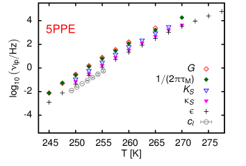
Figure 4: The six characteristic frequencies (based on the four measured quantities) as functions of temperature for 5PPE. Filled symbols ($\tau_{\text{M}}$ and $\kappa_{S}$) indicate a quantity that is not directly measured, but derived from one of the other measured quantities.

Figure 4 shows the characteristic frequencies as functions of temperature online for 5-polyphenyl-4-ether (5PPE) (the figure is equivalent to Fig. 2(a) in the main paper). Note that $\alpha_{l}$ data are not available for 5PPE due to its larger dielectric relaxation strength NissAlpha .

Appendix B Materials and methods

The two substances investigated are both commercial vacuum-pump oils and were used as received without further purification. DC704 (tetramethyl-tetraphenyl-trisiloxane) was required from Aldrich as Dow Corning ® silicone diffusion pump fluid [445975]. 5PPE (5-polyphenyl-4-ether) was required as Santovac ® 5 Polyphenyl ether.

With the exception of $\alpha_{l}(t)$ all quantities were measured in the same cryostat Igarashi2008a ; Igarashi2008b , ensuring the same absolute temperature. The thermal expansion coefficient data were taken in a different cryostat, for which the absolute temperature was calibrated using the liquid’s dielectric relaxation time in a temperature range where data exists from both cryostats. It was not possible to measure $\alpha_{l}$ for 5PPE, because $\alpha_{l}$ was measured by a method that requires a very small dielectric relaxation strength NissAlpha .

Appendix C The perfectly correlating (single-parameter) model liquid

As stated in the main text a strongly correlating liquid Pedersen2008 ; *Bailey2008; *Bailey2008a; *Schroder2009a; *Gnan2009; *Schroder2009; *Pedersen2010; *Gnan2010 is characterized in computer simulations by strong correlations between the constant-volume equilibrium fluctuations of virial and potential energy (correlation coefficient above 0.9). Such a liquid is an approximate single-parameter liquid, i.e., it does not have three independent isotropic thermoviscoelastic response functions, but merely one (to a good approximation)Ellegaard2007 .

The purpose of the model calculation is to investigate to which extent our findings regarding the difference in characteristic frequency between the thermoviscoelastic response functions $c_{l}$, $\alpha_{l}$, and $\kappa_{S}$ are consistent with the hypothesis that the investigated liquid tetramethyl-tetraphenyl-trisiloxane (DC704) is a strongly correlating liquid. For this purpose a perfect single-parameter model liquid is constructed and the loss-peak frequencies of the measured response functions are calculated.

At all frequencies a perfect single-parameter liquid obeysEllegaard2007

$$\frac{T_{0}\alpha_{p}^{\prime\prime}(\omega)}{c_{p}^{\prime\prime}(\omega)}=\gamma_{Tp}=\frac{\kappa_{T}^{\prime\prime}(\omega)}{\alpha_{p}^{\prime\prime}(\omega)}$$ (2)

where $\gamma_{Tp}$ is a constant. By the Kramers-Kronig relations Eq. (2) implies that the relaxation strengths are related by

$$\frac{T_{0}\Delta{\alpha_{p}}}{\Delta{c_{p}}}=\gamma_{Tp}=\frac{\Delta{\kappa_{T}}}{\Delta{\alpha_{p}}}.$$ (3)

It follows that the full response functions can be written as

$$\alpha_{p}(\omega) = \Delta{\alpha_{p}}f(\omega)+\alpha_{p\infty}$$ (4a)

$$c_{p}(\omega) = \frac{T_{0}}{\gamma_{Tp}}\Delta{\alpha_{p}}f(\omega)+c_{p\infty}$$ (4b)

$$\kappa_{T}(\omega) = \gamma_{Tp}\Delta{\alpha_{p}}f(\omega)+\kappa_{T\infty},$$ (4c)

where $f(\omega)$ is a normalized complex susceptibility, defining the common time scale as well as the shape of the relaxation functions. $\alpha_{p\infty}$, $c_{p\infty}$, and $\kappa_{T\infty}$ are the high-frequency limits of the response functions, and $\Delta{\alpha_{p}}$ is the relaxation strength of $\alpha_{p}$.

The measured quantities $c_{l}$, $\alpha_{l}$, and $\kappa_{S}$ are related to those of Eq. (4) by Christensen2007 ; Christensen2008 :

$$\alpha_{l}(\omega) = \frac{\alpha_{p}(\omega)}{1+4/3\;G(\omega)\kappa_{T}(\omega)}$$ (5a)

$$c_{V}(\omega) = c_{p}(\omega)-\frac{T_{0}\alpha_{p}(\omega)^{2}}{\kappa_{T}(\omega)}$$ (5b)

$$\kappa_{S}(\omega) = \frac{c_{V}(\omega)}{c_{p}(\omega)}\kappa_{T}(\omega)$$ (5c)

$$c_{l}(\omega) = \frac{1/\kappa_{S}(\omega)+4/3\;G(\omega)}{1/\kappa_{T}(\omega)+4/3\;G(\omega)}c_{V}(\omega).$$ (5d)

Thus if the shear modulus is known, it is possible to calculate the measured quantities based on the quantities which are related in the single-parameter liquid: $\alpha_{p}$, $c_{p}$, and $\kappa_{T}$.

Table 1: Parameters for the perfect single-parameter liquid mimicking the properties of DC704 at the temperature $214$. The values are based on the data presented in Refs. Gundermann2011, ; HecksherPHD, .

$\gamma_{Tp}$	:	$2.5\cdot 10^{-7}{}^{3}\per$
$\Delta{\alpha_{p}}$	:	$3.2\cdot 10^{-4}1/$
$\alpha_{p\infty}$	:	$1.4\cdot 10^{-4}1/$
$c_{p\infty}$	:	$1.4\cdot 10^{6}\per(^{3})$
$\kappa_{T\infty}$	:	$1.9\cdot 10^{-10}{}^{3}\per$
$G_{\infty}$	:	$3/5\Delta{K_{S}}$
$\log_{10}\left(\frac{\nu_{\text{lp},G}}{\nu_{\text{lp},f}}\right)$	:	1.1
$f(\omega)$	:	$\left({1+\frac{1}{(i\omega\tau)^{-1}+k(i\omega\tau)^{-\alpha}}}\right)^{-1}$
$\alpha$	:	0.44
$k$	:	$1.05$

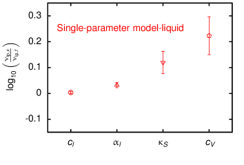
Figure 5: Time-scale index for $c_{l}$, $\alpha_{l}$, $\kappa_{S}$, and $c_{V}$ relative to the loss peak position of the common function $f(\omega)$ entering Eq. (4).

A single-parameter model liquid with properties close to DC704 was constructed in the following way (the parameters used are listed in Table 1) :

• The high-frequency limits and relaxation strengths of $\alpha_{p}$, $c_{p}$, and $\kappa_{T}$ were calculated based on the high- and low-frequency limits of of $c_{l}$, $\kappa_{S}$, $\alpha_{l}$, and $G$ as given in Ref. Gundermann2011, . This can be done, because Eq. (5) can be inverted analytically.

• $\gamma_{Tp}$ was estimated from Eq. (3). DC704 is not a perfectly correlating liquid, so the right- and left-hand sides do not give exactly the same value. They differ by $\approx 10\%$, which is below their respectively uncertainties, and the average was used.

• The normalized complex susceptibility $f(\omega)$ was chosen to follow a “generalized BEL model”, which we found to describe the alpha relaxation in many liquids very well Christensen1994b ; Saglanmak2010 ; Jakobsen2011 :

  $$f(\omega)=\frac{1}{1+\frac{1}{(i\omega\tau)^{-1}+k(i\omega\tau)^{-\alpha}}}.$$ (6)

  The parameters were estimated by fitting a modulus version of the model to the shear modulus data.

• The shear modulus was assumed to follow a modulus version of Eq. (6), having $G_{\infty}=3/5\Delta{K_{S}}$ (in Ref. HecksherPHD, this relation was shown to apply for DC704), and a time scale that is one decade faster than $f(\omega)$ (as seen in Fig. 2 of the main paper).

• $10^{5}$ realizations of the model liquid were calculated with the parameters $\gamma_{Tp}$, $\Delta{\alpha_{p}}$, $\alpha_{p\infty}$, $c_{p\infty}$, and $\kappa_{T\infty}$ chosen independently from Gaussian distributions with mean given as in Table 1 and a standard deviation of $20\%$. This was done in order to investigate the robustness of the results with respect to the influence of the absolute levels. The chosen standard deviation is larger than the estimated uncertainties on the quantities, ensuring that the results represent a “worst case scenario”. For each realization the loss-peak positions of $c_{l}$, $\alpha_{l}$, and $\kappa_{S}$ (and additionally $c_{V}$) were calculated.

Figure 5 shows the time-scale index between the loss-peak frequencies of the calculated quantities with respect to the loss-peak frequency of $f(\omega)$ (Eq. (6)). That is, Fig.  5 shows the loss-peak positions of $c_{l}$, $c_{V}$, $\alpha_{l}$ and $\kappa_{S}$ when the underlying liquid is a perfect single-parameter liquid in which $c_{p}$, $\alpha_{p}$, and $\kappa_{T}$ have the same loss-peak position. It can be seen that the influence on the loss-peak position of measuring the longitudinal specific heat and thermal expansion coefficient, instead of their isobaric counterparts, is very small. Compressibility, on the other hand, is affected more by measuring the adiabatic version instead of the isothermal.

Appendix D Choice of extrapolation function

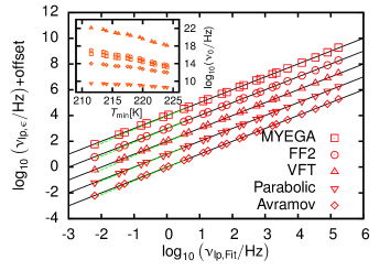
Figure 6: Quality of five fitting functions of the loss-peak frequency as functions of temperature. The main figure shows the result of evaluating fits of the five different function to the full data set (see Table 2 for details on expressions and parameters and the main text for references), plotted against the measured loss-peak frequencies (for clarity the plots have been offset by an integer constant on the y-axis). For a perfect fit the points fall on the shown black lines. The (barely visible) dashed green lines show the ability to extrapolate; it is the result of evaluating a fit including only data down to $\log_{10}(\nu_{\text{lp}})=0.67$ (corresponding to $220$). The insert shows the best fit attack frequencies, $\nu_{0}$, as functions of the lowest temperature included in the fit (see the main text for details). This figures shows that all five functions fit data well, but the Parabolic function is the best function to used for extrapolation of data to lower temperatures.

Table 2: Fitting functions. The table presents the five functions (see main text for references) which were tested for the ability to extrapolate the dielectric loss peak to the temperatures where the thermal expansion coefficient was measured. The parameters reported derive from fitting the full data set. The “Parameter change” is the relative change in the parameters between fitting to the 12 highest temperatures (down to $224$) and to the full set of 24 points (down to $211.5$).

	$\nu_{\text{lp}}(T)$	Parameters	Parameter chage
VFT	$\nu_{0}\exp\left(-\frac{A}{T-T_{0}}\right)$	$A=3510,T_{0}=148.9,\log_{10}(\nu_{0})=22.1$	$A:62\%,T_{0}:-10\%,\log_{10}(\nu_{0}):22\%$
Avramov	$\nu_{0}\exp\left(-\left(\frac{B}{T}\right)^{n}\right)$	$n=5.0,B=437.0,\log_{10}(\nu_{0})=14.0$	$n:-19\%,B:17\%,\log_{10}(\nu_{0}):17\%$
Parabolic	$\nu_{0}\exp\left(-J^{2}\left(\frac{1}{T}-\frac{1}{T_{0}}\right)^{2}\right)$	$J=3740^{2},T_{0}=299.6,\log_{10}(\nu_{0})=9.5$	$J:-8\%,T_{0}:5\%,\log_{10}(\nu_{0}):11\%$
Double exp (MYEGA)	$\nu_{0}\exp\left(-\frac{K}{T}\exp\left(\frac{C}{T}\right)\right)$	$K=294.4,C=722.5,\log_{10}(\nu_{0})=16.2$	$K:344\%,C:-28\%,\log_{10}(\nu_{0}):22\%$
Double exp (FF2)	$\nu_{0}\exp\left(-A\exp\left(\frac{T_{2}}{T}\right)\right)$	$A=0.650,T_{2}=893.5,\log_{10}(\nu_{0})=17.0$	$A:393\%,T_{2}:-25\%,\log_{10}(\nu_{0}):25\%$

In order to extrapolate the dielectric data to the temperatures of the thermal expansion coefficient, a fitting function is needed. Inspired by the work of Elmatad et al. Elmatad2010 five fitting functions were investigated (Table 2): The Vogel-Fulcher-Tammann (VFT) function Vogel1921 ; Fulcher1925 ; Tammann1925 , the Avramov function Litovitz1952 ; Barlow1959 ; Barlow1966 ; Harrison1976 ; Bassler1987 ; Avramov2005 , the Parabolic function Garrahan2003 ; Elmatad2009 ; Elmatad2010 , and two double-exponential functions: The MYEGA function suggested by Mauro et at. Mauro2009 and the similar FF2 function of Hecksher et al. Hecksher2008 . All five functions have three fitting parameters, one of which is the microscopic attack frequency ($\nu_{0}$).

Each function was fitted to the loss-peak position from the dielectric constant, using a least-square minimization. Figure 6 illustrates the quality of the fits, which for all five functions are excellent. The fitting parameters are given in Table 2. In order to explore to which extent the functions are useful for extrapolating, the stability of the parameters were investigated when adding points to the fit. All functions were fitted to the 12 points at the highest temperatures. Points were then added to the data set one by one and the functions re-fitted. The relative change in the fitting parameters from the initial to the final data set is reported in Table 2, and the insert in Fig. 6 shows the fits for the attack frequencies ($\nu_{0}$). A clear convergence of the parameters was not observed for any of the functions, but the Parabolic function has the most stable parameters (however, the Avramov function is only slightly worse and it has a more physically realistic attack frequency). Finally, the ability to extrapolate was investigated by fitting to the first 16 points and then evaluating the fitted function at the lower temperatures, as shown by the dashed green lines in Fig. 6). The extrapolation spans $\approx 2.5$ decade in loss-peak frequency, comparable to the extrapolation needed to get to the lowest temperature of the thermal expansion coefficient. Again the Parabolic function is best, but not perfect. Based on this the Parabolic function was chosen as extrapolation function.