Gravitino Dark Matter and Neutrino Masses in Partial Split Supersymmetry

Abstract

Partial Split Supersymmetry with bilinear R-parity violation allows to reproduce all neutrino mass and mixing parameters. The viable dark matter candidate in this model is the gravitino. We study the hypothesis that both possibilities are true: Partial Split Supersymmetry explains neutrino physics and that dark matter is actually composed of gravitinos. Since the gravitino has a small but non-zero decay probability, its decay products could be observed in astrophysical experiments. Combining bounds from astrophysical photon spectra with the bounds coming from the mass matrix in the neutrino sector we derive a stringent upper limit for the allowed gravitino mass. This mass limit is in good agreement with the results of direct dark matter searches.

I Introduction

Split supersymmetry (SS) was originally proposed to address some of the most conspicuous problems of supersymmetric models, which are fast proton decay and excessive flavor changing neutral currents and CP violation ArkaniHamed:2004fb . In SS the solution to these problems is accomplished by considering all squarks and sleptons very massive, with a mass scale $\widetilde{m}$ somewhere between the supersymmetric scale $M_{susy}$ and the Grand Unification scale $M_{GUT}$. One of the Higgs bosons remains light, as usual in supersymmetric models, as well as the gauginos and higgsinos, with all these particles having a mass accessible to the LHC Aad:2009wy .

If R-Parity violation (RpV) is introduced in supersymmetric models, lepton number and/or baryon number will be violated as well, inducing a potentially too fast proton decay Barbier:2004ez . Nevertheless, in SS the trilinear RpV couplings play little role in the phenomenology, with the exception being in the gluino decay rate. In this case, only bilinear RpV (BRpV) is relevant, opening up the possibility for a neutrino mass generation mechanism, without running into the danger of a too fast proton decay. As in any BRpV model, in SS-BRpV the atmospheric neutrino mass squared difference is generated by a low energy see-saw mechanism due to the mixing between neutrinos and neutralinos Nowakowski:1995dx ; Hirsch:2000ef . Nevertheless, at one loop the only contributions to the neutrino mass matrix, coming from loops with the Higgs boson and neutralinos, is not enough to generate a solar neutrino mass squared difference Chun:2004mu ; Diaz:2006ee . Thus, an additional contribution to the model is needed Diaz:2009yz or the model itself has to be generalized.

In Partial Split Supersymmetry (PSS) all squarks and sleptons have a mass of the order of the SS mass scale $\widetilde{m}$, but both Higgs doublets remain with a mass at the electroweak scale Sundrum:2009gv ; Diaz:2006ee . The addition of RpV to this model was introduced to be able to generate a solar neutrino mass Diaz:2006ee . Loop contributions from neutral CP-even and CP-odd Higgs bosons are indeed able to do the job, producing not only the atmospheric and solar masses, but also the atmospheric, solar, and reactor neutrino mixing angles Diaz:2009gf .

Since R-Parity is not conserved, the lightest supersymmetric particle (LSP) will be unstable and decay into SM particles. This will occur very fast if the LSP is the traditional neutralino, losing it as a candidate for Dark Matter. It is however known that in the case of a gravitino LSP, despite being unstable, it will decay very slowly via gravitationally induced couplings Grefe:2008zz ; Wang:2005at . Suppression of the gravitino interactions by both the Planck mass and the R-parity violating couplings leads to a very long-lived massive particle, whose lifetime can typically be of several orders of magnitude longer than the age of the universe. The next-to-lightest superparticle (NLSP), on the other hand, has a lifetime which is much shorter than 1 second, and thus becomes harmless to a successful big-bang nucleosynthesis Takayama:2000uz .

The fact that the gravitino decays to ordinary particles in such a scenario has given rise to interesting phenomenological studies Ibarra:2007wg ; Ishiwata:2008cu ; Yuksel:2007dr . An important one is the study of the photon spectrum produced from the two-body decay Choi:2009ng ; Buchmuller:2007ui ; Bertone:2007aw , and more recently from the three-body decays of the gravitino Choi:2010jt ; Choi:2010xn . Important constraints on the mass and lifetime of the gravitino can be derived from the fact that its decay has not been detected by gamma-ray telescopes, most importantly the Fermi Large Area Telescope (Fermi LAT) Collaboration:2010gq ; Abdo:2010nz ; Atwood:2009ez ; Abdo:2009mr ; Abdo:2010nc .

Further constraints on the allowed parameters can be derived from the measurements of the neutrino masses and mixing parameters, which in PSS provide constraints on the R-parity violating couplings Diaz:2006ee ; Diaz:2009gf .

In this work we study these two independent constraints, and show that when taken together they imply the existence of a maximal value of the light gravitino mass $m_{3/2}^{max}$, and also the existence of a minimum value of the gravitino lifetime. Our findings are in good agreement with direct dark matter searches Ahmed:2009zw ; Aprile:2011hi which put much stronger constraints on dark matter particles with masses $\gg m_{3/2}^{max}$. It is important to mention that this kind of model can be further studied in the context of the observed Pamela electron/positron excess and direct LHC signals Bajc:2010qj ; Chen:2009ew . Further studies are possible in the context of the early universe Khlopov:1984pf ; Falomkin:1984eu ; Khlopov:2004tn . However, since in our work the gravitino has an extremely long lifetime, the implications from gravitino decay in the early universe are not taken into account.

This model is a bottom up approach, it can however be motivated by a number of general considerations. In ref. ArkaniHamed:2004yi it is shown that a Split Supersymmetric spectrum can be easily generated in models with direct mediation of supersymmetry breaking, i.e., without invoking a hidden sector. In opposition to low energy supersymmetric models, in SS this is possible because the gauginos are allowed to be much lighter than the sfermions. A toy model is given, where sfermion masses are generated at a scale $\widetilde{m}$ while gaugino masses are induced at a lower scale $\mu$, after integrating out physics at a higher scale that controls the supersymmetry breaking. In the same model, a gravitino mass is generated at the scale $\widetilde{m}^{2}/M_{Pl}$ allowing it to be even lighter than gauginos. This toy model generates also a $B_{\mu}$ term of the order of $\widetilde{m}^{2}$ and it would have to be modified in order to accommodate PSS, where $B_{\mu}$ is required to be much smaller than $\widetilde{m}^{2}$. It is worth to mention that a $B_{\mu}\ll\widetilde{m}^{2}$ would alleviate the otherwise present fine-tuning needed in the Higgs potential to generate a correct electroweak symmetry braking Drees:2005cp . As a top down approach to PSS we mention also ref. Sundrum:2009gv where a PSS spectrum is given. In this model sfermions masses are generated at a scale $\widetilde{m}^{2}\sim V_{0}/M^{2}$, where supersymmetry breaking originates with a hidden sector dynamics with vacuum energy $V_{0}$, and it is communicated to the visible sector by massive fields of mass $M$. In addition, two light Higgs scalars are composite with a mass $m_{h}\sim\frac{g}{4\pi}\Lambda_{comp}$, with $\Lambda_{comp}$ the typical scale of the strong dynamics. The gravitino mass is of the order $\sqrt{V_{0}}/M_{Pl}$ and can be the LSP for values for example $V_{0}\sim(10^{9}\,{\mathrm{GeV}})^{4}$.

II Partial Split Supersymmetry

In PSS both Higgs doublets remain with a mass at the electroweak scale. As it happens in SS, higgsinos, gauginos, and Higgs bosons interact via induced couplings of the type,

$${\cal L}_{PSS}^{RpC} \owns -\textstyle{\frac{1}{\sqrt{2}}}H_{u}^{\dagger}(\tilde{g}_{u}\sigma\widetilde{W}+\tilde{g}^{\prime}_{u}\widetilde{B})\widetilde{H}_{u}-\textstyle{\frac{1}{\sqrt{2}}}H_{d}^{\dagger}(\tilde{g}_{d}\sigma\widetilde{W}-\tilde{g}^{\prime}_{d}\widetilde{B})\widetilde{H}_{d}+\mathrm{h.c.},$$ (1)

where $\tilde{g}_{u}$, $\tilde{g}^{\prime}_{u}$, $\tilde{g}_{d}$, and $\tilde{g}^{\prime}_{d}$ are couplings induced in the effective low energy lagrangian. At the SS scale $\widetilde{m}$ they satisfy the boundary conditions,

$$\tilde{g}_{u}=\tilde{g}_{d}=g\,,\qquad\tilde{g}^{\prime}_{u}=\tilde{g}^{\prime}_{d}=g^{\prime},$$ (2)

evolving with independent RGE down to the electroweak scale. Similarly to the MSSM, both Higgs fields acquire a vacuum expectation value $\langle H_{u}\rangle=v_{u}$ and $\langle H_{d}\rangle=v_{d}$, with the constraint $v^{2}=v_{u}^{2}+v_{d}^{2}=246\,{\mathrm{GeV}}^{2}$ and the definition $\tan\beta=v_{u}/v_{d}$. Gauginos and higgsinos mix forming the neutralinos, with a mass matrix very similar to the one in the MSSM,

$${M}_{\chi^{0}}=\left[\begin{array}[]{cccc}M_{1}&0&-\frac{1}{2}\tilde{g}^{\prime}_{d}c_{\beta}v&\frac{1}{2}\tilde{g}^{\prime}_{u}s_{\beta}v\\ 0&M_{2}&\frac{1}{2}\tilde{g}_{d}c_{\beta}v&-\frac{1}{2}\tilde{g}_{u}s_{\beta}v\\ -\frac{1}{2}\tilde{g}^{\prime}_{d}c_{\beta}v&\frac{1}{2}\tilde{g}_{d}c_{\beta}v&0&-\mu\\ \frac{1}{2}\tilde{g}^{\prime}_{u}s_{\beta}v&-\frac{1}{2}\tilde{g}_{u}s_{\beta}v&-\mu&0\end{array}\right],$$ (3)

where $M_{1}$ and $M_{2}$ are the gaugino masses associated to the $U(1)$ and $SU(2)$ gauge bosons, and $\mu$ is the higgsino mass. In our calculations we will neglect the running of the higgsino-higgs-gaugino couplings and work with their approximated value indicated by eq. (2).

The addition of R-Parity violation to the PSS lagrangian allows us to study a mechanism for neutrino mass generation. Trilinear couplings are not relevant for this problem, because all squarks and sleptons are very heavy, with a mass of the order of $\widetilde{m}$, and thus decoupled from the low energy effective theory. Only BRpV is relevant, and is described by the terms,

$${\cal L}_{PSS}^{RpV}=-\epsilon_{i}\widetilde{H}_{u}^{T}\epsilon L_{i}\ -\ \textstyle{\frac{1}{\sqrt{2}}}b_{i}H_{u}^{T}\epsilon(\tilde{g}_{d}\sigma\widetilde{W}-\tilde{g}^{\prime}_{d}\widetilde{B})L_{i}\ +\ h.c.,$$ (4)

where $\epsilon=i\sigma_{2}$. The $\epsilon_{i}$ are the supersymmetric BRpV parameters in the superpotential, which at the low scale manifest themselves as mixing between higgsinos and lepton fields. The $b_{i}$ are three dimensionless parameters attached to lepton-higgs-gaugino interactions. They are analogous to the ones in eq. (1), except that violate R-Parity, and are generated in the effective low energy theory.

The origin of the BRpV terms in (4) is related to the $\mu$-problem which refers to the origin of the term $\mu H_{u}H_{d}$ in the superpotential. As discussed for example in ref. Allanach:2003eb , the same mechanism that solve the $\mu$-problem could be used to explain the origin of the $\epsilon$ terms. A popular mechanism is the existence of non renormalizable couplings of the sort $(a/M_{Pl})\Phi_{1}\Phi_{2}H_{u}H_{d}$, with $a$ being a dimensional constant and $\Phi_{1}$ and $\Phi_{2}$ two hidden sector scalars. When supersymmetry breaks and $\Phi_{1}$ and $\Phi_{2}$ acquire vacuum expectation values a $\mu$-term is generated. Similar terms $(a_{i}/M_{Pl})\Phi_{3}\Phi_{4}H_{u}L_{i}$ can be present generating $\epsilon$-terms, although $a_{i}$ and/or $\langle\Phi_{3}\rangle$, $\langle\Phi_{4}\rangle$ should be much smaller than $a$ and/or $\langle\Phi_{1}\rangle$, $\langle\Phi_{2}\rangle$ in order to have $\epsilon_{i}$ a few order of magnitude smaller than $\mu$, necessary for neutrino physics. The $b_{i}$ terms are generated after integrating out the sleptons, and appear because above the scale $\widetilde{m}$ the Higgs bosons mix with sleptons. At the scale $\widetilde{m}$ we have $b_{i}\sim v_{i}/v_{u}$, with the necessary condition $v_{u}B_{\epsilon i}\sim v_{i}M_{Li}^{2}$ from the minimization of the scalar potential Diaz:2006ee . Large $B_{\epsilon i}$ can be easily obtained in a similar way as for $B_{\mu}$, as explained in ArkaniHamed:2004yi . We mention also ref. FileviezPerez:2010ek where R-Parity is naturaly broken radiatively when a right-handed sneutrino acquires a vacuum expectation value, generating bilinear R-Parity violating terms. In our work, we concentrate on the effect of bilinear R-Parity violation. Trilinear R-Parity violating couplings could be present, but we ignore their effects due to the large mass of the sfermions.

III Neutrino masses

When Higgs bosons acquire vacuum expectation values, mixing terms between gauginos and leptons are generated, producing the following mixing between neutrinos and heavier fermions,

$${\cal L}^{RpV}_{PSS}=-\left[\epsilon_{i}\widetilde{H}_{u}^{0}+\frac{1}{2}b_{i}v_{u}\left(\tilde{g}_{d}\widetilde{W}_{3}-\tilde{g}^{\prime}_{d}\widetilde{B}\right)\right]\nu_{i}\ +\ h.c.\ +\ \ldots$$ (5)

The effect of these terms is that neutralinos mix with neutrinos, forming a $7\times 7$ mass matrix, which in the basis $\left(\widetilde{B},\widetilde{W},\widetilde{H}_{u},\widetilde{H}_{d},\nu_{e},\nu_{\mu},\nu_{\tau}\right)$ has the form,

$${\cal M}_{N}=\left[\begin{array}[]{cc}M_{\chi^{0}}&m^{T}\\ m&0\end{array}\right],$$ (6)

and where the $4\times 4$ submatrix $M_{\chi^{0}}$ is the neutralino mass matrix in eq. (3). The $4\times 3$ neutralino-neutrino mixing block

$$m=\left[\begin{array}[]{cccc}-\frac{1}{2}\tilde{g}^{\prime}_{d}b_{1}v_{u}&\frac{1}{2}\tilde{g}_{d}b_{1}v_{u}&0&\epsilon_{1}\cr-\frac{1}{2}\tilde{g}^{\prime}_{d}b_{2}v_{u}&\frac{1}{2}\tilde{g}_{d}b_{2}v_{u}&0&\epsilon_{2}\cr-\frac{1}{2}\tilde{g}^{\prime}_{d}b_{3}v_{u}&\frac{1}{2}\tilde{g}_{d}b_{3}v_{u}&0&\epsilon_{3}\end{array}\right],$$ (7)

develops from terms in eq. (5). A diagonalization by blocks of the mass matrix in eq. (6) can be achieved by a rotation $\mathcal{N}\mathcal{M}_{N}\mathcal{N}^{T}$ given by,

$$\mathcal{N}\simeq\begin{bmatrix}N&N\xi^{T}\\ -\xi&1\end{bmatrix},$$ (8)

where we define,

$$\xi=mM_{\chi^{0}}^{-1},$$ (9)

with

$$\xi_{i1} = \frac{\tilde{g}^{\prime}_{d}\,\mu M_{2}}{2\det{M_{\chi^{0}}}}\Lambda_{i}$$

$$\xi_{i2} = -\frac{\tilde{g}_{d}\,\mu M_{1}}{2\det{M_{\chi^{0}}}}\Lambda_{i}$$ (10)

$$\xi_{i3} = \frac{v_{u}}{4\det{M_{\chi^{0}}}}\left(M_{1}\tilde{g}_{u}\tilde{g}_{d}+M_{2}\tilde{g}^{\prime}_{u}\tilde{g}^{\prime}_{d}\right)\Lambda_{i}-\frac{\epsilon_{i}}{\mu}$$

$$\xi_{i4} = -\frac{v_{d}}{4\det{M_{\chi^{0}}}}\left(M_{1}\tilde{g}^{2}_{d}+M_{2}\tilde{g}^{\prime 2}_{d}\right)\Lambda_{i}$$

and $\Lambda_{i}=\mu b_{i}v_{u}+\epsilon_{i}v_{d}$. This leaves an induced effective neutrino mass matrix equal to,

$${\bf M}_{\nu}^{(0)}|_{ij}=-m^{T}{\mathrm{M}}_{\chi^{0}}^{-1}m|_{ij}=A^{(0)}\Lambda_{i}\Lambda_{j},$$ (11)

with

$$A^{(0)}=\frac{M_{1}\tilde{g}^{2}_{d}+M_{2}\tilde{g}^{\prime 2}_{d}}{4\det{M_{\chi^{0}}}}.$$ (12)

At this level only one neutrino acquires mass, leaving the solar squared mass difference null and the solar angle undetermined. Quantum corrections contribute to the neutrino mass matrix in such a way that the degeneracy in eq. (11) is lifted, leaving it with the following form,

$${\bf M}_{\nu}|_{ij}=A\Lambda_{i}\Lambda_{j}+C\epsilon_{i}\epsilon_{j},$$ (13)

where the $B$ term Diaz:2009gf has been made to vanish by an appropriate choice of the subtraction point. Thus at one loop two neutrinos acquire a mass while the third one remains massless. Since in this case the experimental value $\Delta m^{2}_{sol}/\Delta m^{2}_{atm}\approx 0.035$ implies $m_{\nu_{3}}\gg m_{\nu_{2}}$ we have,

$$\Delta m^{2}_{atm} \approx \left(A|\vec{\Lambda}|^{2}+C|\vec{\epsilon}\,|^{2}\right)^{2}-2AC|\vec{\Lambda}\times\vec{\epsilon}|^{2},$$

$$\Delta m^{2}_{sol} \approx \frac{A^{2}C^{2}|\vec{\Lambda}\times\vec{\epsilon}\,|^{4}}{\left(A|\vec{\Lambda}|^{2}+C|\vec{\epsilon}|^{2}\right)^{2}}.$$ (14)

For later use, we introduce the photino $\widetilde{\gamma}$ and zino $\widetilde{Z}$ fields by rotating by the weak mixing angle the weakly interacting gauginos $\tilde{B},\tilde{W}$, in direct analogy to their standard model counter parts

$$\left(\begin{array}[]{c}\widetilde{\gamma}\\ \widetilde{Z}^{0}\\ \dots\end{array}\right)=\left(\begin{array}[]{ccc}c_{W}&s_{W}\dots\\ -s_{W}&c_{W}\dots\\ \dots&\dots\end{array}\right)\left(\begin{array}[]{c}\widetilde{B}\\ \widetilde{W}\\ \dots\end{array}\right)=A_{W}\left(\begin{array}[]{c}\widetilde{B}\\ \widetilde{W}\\ \dots\end{array}\right),$$ (15)

where the dots indicate that all other states are just multiplied by the unit matrix. Thus when dealing with this new basis $\left(\widetilde{\gamma},\widetilde{Z^{0}},\widetilde{H}_{u},\widetilde{H}_{d},\nu_{e},\nu_{\mu},\nu_{\tau}\right)$ the mixing matrix is

$$\mathcal{N}^{\prime}=\mathcal{N}A_{W}^{T}\quad,$$ (16)

where only the first two states are rotated.

IV Gravitino Decay

Indirect observation of the gravitino becomes a possibility due to its decay to ordinary particles. In this section we calculate the possible decay channels of the gravitino as dark matter candidate, assuming that $m_{3/2}<m_{W}$. We then relate these results to experimental bounds on the decay products and on the RpV parameters.

IV.1 Two-body decay

When R-parity is conserved the gravitino can radiatively decay into a photon via the following term in the Lagrangian,

$${\cal L}\owns-\frac{1}{4M_{P}}\overline{\psi}_{\mu}\sigma^{\nu\rho}\gamma^{\mu}\lambda_{\gamma}F_{\nu\rho}$$ (17)

where $M_{P}$ is the Planck mass, $\psi_{\mu}$ is the spin-$3/2$ gravitino field, $\lambda_{\gamma}$ is the spin-$1/2$ photino field, $F_{\nu\rho}=\partial_{\nu}A_{\rho}-\partial_{\rho}A_{\nu}$ is the photon field strength, and $A_{\mu}$ is the photon field. This coupling might in principle be modified by a factor of order one. In this work however we assume that (17) is the exact form of the coupling. Variations of the final result can then be studied by order one shifts of the Planck mass $M_{P}$. This Lagrangian term induces the following decay,

$=-\,i\,{\cal M}_{0}$

where the cross indicates we are picking the photino component of the corresponding neutrino, which mix due to violation of R-Parity. The amplitude for this decay is

$${\cal M}_{0}=-\frac{i}{4M_{P}}\Big{\{}\overline{\nu}(q,s)\gamma^{\mu}\big{[}/\!\!\!k,\gamma^{\nu}\big{]}\psi_{\mu}(p,\lambda)\Big{\}}\epsilon_{\mu}(k,m)\,{U}_{\widetilde{\gamma}\nu},$$ (18)

where ${U}_{\widetilde{\gamma}\nu}$ is the amount of photino in the neutrino fields, as indicated by the neutrino eigenvector. We write the gravitino field as the tensor product of a spin-1/2 field with a spin-1 field,

$$\psi_{\mu}(p,\lambda)=\sum_{s,m}\langle 1/2,s;1,m|3/2,\lambda\rangle u(p,s)\epsilon_{\mu}(p,m),$$ (19)

obtaining the following completeness relation Grefe:2008zz ,

$$\sum_{\lambda}\psi_{\mu}(p,\lambda)\overline{\psi}_{\nu}(p,\lambda)=-(/\!\!\!p-m_{3/2})\Bigg{[}\bigg{(}g_{\mu\nu}-\frac{p_{\mu}p_{\nu}}{m_{3/2}^{2}}\bigg{)}-\frac{1}{3}\bigg{(}g_{\mu\sigma}-\frac{p_{\mu}p_{\sigma}}{m_{3/2}^{2}}\bigg{)}\bigg{(}g_{\nu\lambda}-\frac{p_{\nu}p_{\lambda}}{m_{3/2}^{2}}\bigg{)}\gamma^{\sigma}\gamma^{\lambda}\Bigg{]}.$$ (20)

Knowing the above relation, the calculation of the differential cross section is standard, giving the result

$$\frac{d\Gamma}{dE_{\gamma}d\Omega}=\frac{\langle|{\cal{M}}_{0}|^{2}\rangle}{64\pi^{2}m_{3/2}}\delta\left(E_{\gamma}-\frac{m_{3/2}}{2}\right)=\frac{m_{3/2}^{3}}{128\pi^{2}M_{P}^{2}}|{U}_{\widetilde{\gamma}\nu}|^{2}\delta\left(E_{\gamma}-\frac{m_{3/2}}{2}\right),$$ (21)

which is independent of the angles as expected. The total decay rate is then

$$\Gamma(\widetilde{G}\rightarrow\gamma\nu)=\frac{m_{3/2}^{3}}{32\pi M_{P}^{2}}|{U}_{\widetilde{\gamma}\nu}|^{2}.$$ (22)

For a gravitino mass $m_{3/2}<m_{W}$ this is the only kinematically allowed 2-body decay. By using the relation in eq. (16) one finds that the photino-neutrino mixing factor in PSS is

$$U_{\widetilde{\gamma}\nu_{i}}=\mathcal{N}_{i1}c_{W}+\mathcal{N}_{i2}s_{W},$$ (23)

with $i=5,6,7$ labeling the neutrino generation, and where $t_{W}=g^{\prime}/g$ is the tangent of the weak mixing angle. Using equations (8) to (10) we find,

$$U_{\widetilde{\gamma}\nu_{i}}\simeq\frac{\mu}{2({\rm det}M_{\chi^{0}})}\left(\tilde{g}_{d}M_{1}s_{W}-\tilde{g}^{\prime}_{d}M_{2}c_{W}\right)\Lambda_{i}.$$ (24)

For the numerical calculations we will require the sum over the generations of the square of the mixing factor:

$$|U_{\widetilde{\gamma}\nu}|^{2}:=\sum_{i}U_{\widetilde{\gamma}\nu_{i}}^{2}\simeq\frac{\mu^{2}}{4({\rm det}M_{\chi^{0}})^{2}}\left(\tilde{g}_{d}M_{1}s_{W}-\tilde{g}^{\prime}_{d}M_{2}c_{W}\right)^{2}|\vec{\Lambda}|^{2}.$$ (25)

This is because we do not distinguish the different neutrino flavors.

IV.2 Three-body decays

When studying the three body decay a more general part of the interaction Lagrangian comes into play

$${\mathcal{L}} \owns -\frac{i}{\sqrt{2}M_{P}}\left[(D^{*}_{\mu}\phi^{i*})\bar{\psi}_{\nu}\gamma^{\mu}\gamma^{\nu}P_{L}\chi^{i}-(D_{\mu}\phi^{i})\bar{\chi}^{i}P_{R}\gamma^{\nu}\gamma^{\mu}\psi_{\nu}\right]$$

$$-\frac{i}{8M_{P}}\bar{\psi}_{\mu}\left[\gamma^{\nu},\gamma^{\rho}\right]\gamma^{\mu}\lambda^{(\alpha)a}F_{\nu\rho}^{(\alpha)a}\quad,$$

where the second line is in analogy to (17) and the first line introduces additional couplings with scalar fields $\phi$. The 3-body decays of the gravitino were studied in detail for the first time in Choi:2010jt ; Choi:2010xn , where explicit formulae are given. Nevertheless, our calculations have yielded that the three-body results in Choi:2010jt have to be corrected. We agree, however, with the conclusion that the 3-body decays are indeed important, and cannot be neglected. We find 3-body decay branching ratios of the order of $10\%$ for gravitino masses of order 10 GeV, and greater for larger masses. The exact formulas for the amplitudes of the contributing diagrams are given in the Appendix.

First we consider the gravitino decay into a fermion pair and a neutrino. The first pair of diagrams are three-body decays via an intermediate photon and $Z$ boson,

$=-\,i\,{\cal M}_{1,2}$

where the cross means we take the photino (or zino) component in the neutrino field. These two amplitudes are equal to,

$${\cal M}_{1} = i\frac{-i}{k^{2}}\overline{u}(k_{1})(-iq_{f})\gamma_{\mu}v(k_{2})\overline{u}(q)\frac{-iU_{\widetilde{\gamma}\nu}}{4M_{P}}\gamma^{\alpha}(k\!\!\!/\gamma^{\mu}-\gamma^{\mu}k\!\!\!/)\psi_{\alpha}(p),$$ (27)

$${\cal M}_{2} = i\frac{-i}{(k^{2}-m_{Z}^{2})+im_{Z}\Gamma_{Z}}\overline{u}(k_{1})\frac{-ig}{c_{W}}\gamma_{\mu}(c_{V}^{f}+c_{A}^{f}\gamma_{5})v(k_{2})\overline{u}(q)\frac{-iU_{\widetilde{Z}\nu}}{4M_{P}}\gamma^{\alpha}(k\!\!\!/\gamma^{\mu}-\gamma^{\mu}k\!\!\!/)\psi_{\alpha}(p),$$

with $c_{V}^{f}=T_{3}^{f}/2-q_{f}s_{W}^{2}$ and $c_{A}^{f}=-T_{3}^{f}/2$. Their contribution to the decay rate is given in the Appendix. The photino-neutrino mixing is given in eq. (24), while an analogous calculation for the zino-neutrino mixing gives,

$$U_{\widetilde{Z}\nu_{i}}\simeq-\frac{\mu}{2({\rm det}M_{\chi^{0}})}\left(\tilde{g}_{d}M_{1}c_{W}+\tilde{g}^{\prime}_{d}M_{2}s_{W}\right)\Lambda_{i}.$$ (28)

To the previous two amplitudes we add a contribution coming from quartic couplings between the gravitino, a gauge boson, and a scalar with its fermionic partner, with the scalar acquiring a vacuum expectation value,

$=-\,i\,{\cal M}_{3}$

The first amplitude is proportional to $b_{i}v_{u}$ and the second to $v_{d}(\epsilon_{i}/\mu)$, in such a way that the combined amplitude ${\cal M}_{3}$ is proportional to $\Lambda_{i}$,

$${\cal M}_{3}=i\frac{-i}{(k^{2}-m_{Z}^{2})+im_{Z}\Gamma_{Z}}\overline{u}(k_{1})\frac{-ig}{c_{W}}\gamma_{\mu}(c_{V}^{f}+c_{A}^{f}\gamma_{5})v(k_{2})\overline{u}(q)\frac{-ig\Lambda_{i}}{4c_{W}\mu M_{P}}P_{R}\gamma^{\alpha}\gamma^{\mu}\psi_{\alpha}(p)\quad.$$ (29)

whose contribution to the decay rate is also given in the Appendix. Since the neutrino is not directly detected, a sum over flavors must be done [as in eq. (25)], after which it is clear that the decay rate will satisfy $\Gamma(\widetilde{G}\rightarrow f\overline{f}\nu)\propto|\vec{\Lambda}|^{2}$.

Now we consider the gravitino decay into two fermions and a charged lepton. The decay via a $W$ gauge boson is represented by the Feynman diagram

$=-\,i\,{\cal M}_{4}$

whose amplitude can be shown to be,

$${\cal M}_{4}=i\frac{-i}{(k^{2}-m_{W}^{2})+im_{W}\Gamma_{W}}\overline{u}(k_{1})\frac{-ig}{2\sqrt{2}}\gamma_{\mu}(1-\gamma_{5})v(k_{2})\overline{u}(q)\frac{-iU_{\widetilde{W}\ell}}{4M_{P}}\gamma^{\alpha}(k\!\!\!/\gamma^{\mu}-\gamma^{\mu}k\!\!\!/)\psi_{\alpha}(p).$$

Its contribution to the decay rate is given in the Appendix, and it is proportional to the wino mixing to charged leptons, given by,

$$U_{\widetilde{W}\ell_{i}}\simeq-\frac{\tilde{g}_{d}}{\sqrt{2}({\rm det}M_{\chi^{+}})}\Lambda_{i},$$ (30)

where $M_{\chi^{+}}$ is the chargino mass matrix Diaz:2006ee . This graph is complemented by an amplitude coming from quartic couplings between the gravitino, a $W$ gauge boson, and a neutral scalar with its charged fermionic partner, with the scalar acquiring a vacuum expectation value,

$=-\,i\,{\cal M}_{5}$

As before, the first amplitude is proportional to $b_{i}v_{u}$ and the second to $v_{d}(\epsilon_{i}/\mu)$, such that the combined amplitude ${\cal M}_{5}$ is proportional to $\Lambda_{i}$,

$${\cal M}_{5}=i\frac{-i}{(k^{2}-m_{W}^{2})+im_{W}\Gamma_{W}}\overline{u}(k_{1})\frac{-ig}{2\sqrt{2}}\gamma_{\mu}(1-\gamma_{5})v(k_{2})\overline{u}(q)\frac{-ig\Lambda_{i}}{2\sqrt{2}\mu M_{P}}P_{R}\gamma^{\alpha}\gamma^{\mu}\psi_{\alpha}(p).$$ (31)

Its contribution to the decay rate is also given in the Appendix. Note that when fermion $f$ is a charged lepton and $f^{\prime}$ is a neutrino, we get interference between diagrams ${\cal M}_{1,2,3}$ in one hand and ${\cal M}_{4,5}$ in the other. This is because the decay $\widetilde{G}\rightarrow\ell^{+}_{i}\ell^{-}_{i}\nu_{j}$ can proceed via a $Z$ or a $W$ gauge boson. In addition, note that $\Gamma(\widetilde{G}\rightarrow f\overline{f}^{\prime}\ell^{-}_{i})=\Gamma(\widetilde{G}\rightarrow f^{\prime}\overline{f}\ell^{+}_{i})$, thus we multiply the first one by two.

The decay rate for the 3-body decays of a gravitino can be written as a sum of the various terms given in the Appendix. We sum over three generations, and neglect the masses of the final states. The end result is proportional to $|\vec{\Lambda}|^{2}$. Thus, in the branching ratio the factor $|\vec{\Lambda}|^{2}$ cancels, depending only on $M_{1}$, $M_{2}$, and the gravitino mass $m_{3/2}$ Choi:2010jt . Here we work with the assumption $M_{2}\simeq 2M_{1}$. The result is shown in Fig. 1, where we plot the branching ratio as a function of $m_{3/2}$ for the three values of $M_{1}=$ 100, 300, and 500 GeV. One observes that the three-body decay becomes important for large gravitino masses $m_{3/2}$ and large $M_{1}$.

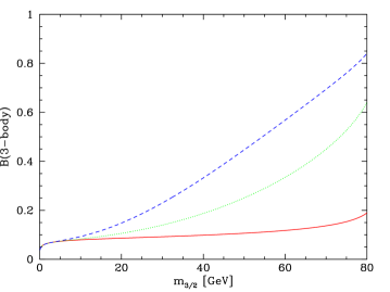
Figure 1: Branching ratio of the three-body decay of the gravitino as a function of its mass $m_{3/2}$, red (full line) for $M_{1}=100\,$GeV, green (dotted line) for $M_{1}=300\,$GeV, and blue (dashed line) for $M_{1}=500\,$GeV.

The dependency on $m_{3/2}$ can be understood as a phase-space effect in the three-body decay rate. The influence of $M_{1}$ on the branching ratio can be understood by the fact that the two-body and three-body decays, by the virtue of the mixings $U_{\tilde{\gamma}\nu}$ and $U_{\tilde{Z}\nu}$ respectively, get suppressed by growing $M_{1}$. In contrast the parts of the three-body decays that contain vacuum expectation values $\langle\tilde{\nu}_{i}\rangle$ and $\langle H_{d}\rangle$ do not experience this suppression and thus become more important in the regime of large $M_{1}$. Those effects are also present in Choi:2010jt , it is only the form of the curves that turned out to change in the corrected version. For the masses we are interested here, $m_{3/2}\>\raisebox{-2.15277pt}{$\stackrel{{\scriptstyle\textstyle<}}{{\sim}}$}\>10$ GeV, the 3-body decay is $\>\raisebox{-2.15277pt}{$\stackrel{{\scriptstyle\textstyle<}}{{\sim}}$}\>10\%$ and with small dependence on the gaugino mass. For larger gravitino masses the branching ratio can be as large as $80\%$. Since the calculations are being carried out in the Feynman gauge, there are in principle also diagrams containing Goldstone bosons in the propagator. However, due to the coupling of the Goldstone bosons, those contributions vanish in the limit of light fermion masses.

IV.3 Induced photon flux

The photon spectrum produced by the decay of the gravitino consists of a mono-energetic line of energy $m_{3/2}/2$ from the two-body decay, plus a continuum distribution from the three-body decays. The exact form of the spectrum, which depends on $m_{3/2}$ and $M_{1}$, was studied in detail in Choi:2010jt ; Choi:2010xn using an event generator. Here we are interested in obtaining constraints on the gravitino parameters, for which it suffices as an approximation to consider only the photon line from the two-body decay, as this is the most prominent feature of the spectrum for values of $M_{1}$ up to 1 TeV Choi:2010jt . Including the three-body decay would make our final conclusions slightly more stringent.

The observed spectrum is calculated from the flux of gamma-rays expected at earth. This flux is the sum of two contributions, one from the gravitinos decaying in the galactic halo, and one from the gravitinos decaying at cosmological distances. It has been shown that the first contribution is highly dominant, and so we will neglect the second one Buchmuller:2007ui . In this way the differential flux, as a function of the photon energy $E$, has the following simple form Bertone:2007aw ; Buchmuller:2007ui :

$$E^{2}\frac{dJ_{\rm{halo}}}{dE}=\frac{D_{\gamma}m_{3/2}}{2}\delta\left(E-\frac{m_{3/2}}{2}\right),$$ (32)

with

$$D_{\gamma}=\frac{\Gamma(\widetilde{G}\rightarrow\gamma\nu)}{8\pi}\left\langle\int_{\rm{l.o.s.}}\rho_{\rm{halo}}(\vec{r})d\ell\right\rangle=d_{\gamma}\Gamma(\widetilde{G}\rightarrow\gamma\nu).$$ (33)

The constant $d_{\gamma}$ depends on the dark matter density profile of the halo, and on the region of the sky considered for averaging the flux (denoted by the term in brackets above, where l.o.s. means line of sight). Using the Navarro-Frenk-White profile Navarro:1995iw , and considering the region $|b|\geq 10^{\circ}$ for the average (with $b$ denoting the latitude in galactic coordinates), we find

$$d_{\gamma}=0.80\times 10^{24}~{}~{}[{\rm{MeV~{}cm^{-2}~{}str^{-1}}}].$$ (34)

This region of the sky was the one considered by the Fermi LAT collaboration in the derivation of the extragalactic diffuse spectrum Abdo:2010nz .

V Limits and Constraints

V.1 Constraint from the observed photon spectrum

The fact that the line produced by the gravitino two-body decay has not been observed gives constraints on the mass and the lifetime of the gravitino. Assuming that the extragalactic diffuse spectrum measured by Fermi LAT can be correctly modeled in terms of known sources Collaboration:2010gq , one can use this spectrum to find constraints Abdo:2010nz ; Buchmuller:2009xv .

After the convolution between the calculated flux in eq. (32) and a Gaussian distribution we find

$$E^{2}\frac{dJ_{\rm{halo}}}{dE}=\frac{D_{\gamma}m_{3/2}}{2}\frac{1}{\sqrt{2\pi\sigma^{2}}}e^{-(E-m_{3/2}/2)^{2}/2\sigma^{2}},$$ (35)

where $\sigma$ is related to the energy-dependent resolution of the Fermi LAT instrument $p$ evaluated at the 2-body peak

$$\sigma=pE=p\frac{m_{3/2}}{2}\quad.$$ (36)

The energy dependence of $p$ evaluated at $E=m_{3/2}/2$ can be approximated by Atwood:2009ez ; web

$$p(m_{3/2})=0.349-0.142\log\left(\frac{m_{3/2}}{2~{}{\rm MeV}}\right)+0.019\log^{2}\left(\frac{m_{3/2}}{2~{}{\rm MeV}}\right).$$ (37)

Thus, the maximum of the photon spectrum is given by

$$\left(E^{2}\frac{dJ_{\rm{halo}}}{dE}\right)_{\rm{max}}=\frac{D_{\gamma}}{p(m_{3/2})\sqrt{2\pi}}$$ (38)

On the other hand, the intensity or the integrated flux for the extragalactic diffuse emission (for the range $E>100$ MeV and the sky region $|b|\geq 10^{\circ}$) was measured by the Fermi LAT collaboration Abdo:2010nz ,

$$I(>100~{}{\rm{MeV}})=\int_{100}^{\infty}\,\frac{dJ}{dE}=(1.03\pm 0.17)\times 10^{-5}~{}[\rm{cm^{-2}~{}s^{-1}~{}str^{-1}}].$$ (39)

together with the observation that the spectrum can be fitted by a power law $dJ/dE\propto E^{-\gamma}$, with index $\gamma=2.41\pm 0.05$. From this we calculate the spectrum to be

$$E^{2}\frac{dJ}{dE}=(9.6\pm 1.6)\times 10^{-3}~{}[{\rm MeV~{}cm^{-2}~{}s^{-1}~{}str^{-1}}]~{}\left(\frac{E}{1~{}{\rm{MeV}}}\right)^{2-\gamma},$$ (40)

where the error was directly calculated from the error in the integrated flux using eq. (39).

As we mentioned before, we assume that the central value of the spectrum can be explained by models of known sources Collaboration:2010gq . We impose that the extra contribution from the gravitino source is smaller than a $3\sigma$ error margin. This gravitino contribution is related to the decay rate $\Gamma(\widetilde{G}\rightarrow\gamma\nu)$ through eqs. (33) and (38). By introducing the total decay width, $\tau_{3/2}^{-1}=\Gamma(\widetilde{G}\rightarrow\gamma\nu)+\Gamma(\mathrm{3-body})$, we find the following restriction on the gravitino lifetime,

$$\left(\frac{\tau_{3/2}}{10^{27}~{}{\rm s}}\right)>\frac{0.851}{p(m_{3/2})}B(\widetilde{G}\rightarrow\gamma\nu)\left(\frac{m_{3/2}}{1~{}{\rm GeV}}\right)^{\gamma-2},$$ (41)

where $B(\widetilde{G}\rightarrow\gamma\nu)$ denotes the branching ratio of the 2-body decay. In this way eq. (41) defines a region in the $m_{3/2}-\tau_{3/2}$ plane consistent with the non-observation of the gravitino decay by Fermi LAT.

The gravitino 2-body decay width $\Gamma(\widetilde{G}\rightarrow\gamma\nu)$ is given in eq. (22). If we sum over all neutrino species it becomes proportional to $|\vec{\Lambda}|^{2}$, via $|U_{\widetilde{\gamma}\nu}|^{2}$ in eq. (25). The 3-body decay width is also proportional to $|\vec{\Lambda}|^{2}$. The reasons are analogous to the 2-body decay, since after summing over lepton generations we see that $|{\cal M}_{1}|^{2}$ is proportional to $|U_{\widetilde{\gamma}\nu}|^{2}$, $|{\cal M}_{2}|^{2}$ is proportional to $|U_{\widetilde{Z}\nu}|^{2}$ [eq. (28)], and $|{\cal M}_{4}|^{2}$ is proportional to $|U_{\widetilde{W}\ell}|^{2}$ [eq. (30)]. In addition, amplitudes $|{\cal M}_{3}|^{2}$ and $|{\cal M}_{5}|^{2}$ are directly proportional to $|\vec{\Lambda}|^{2}$ as can be seen from eqs. (29) and (31). In this way, the gravitino lifetime becomes large for two reasons, because the Planck mass is large and because BRpV is small: $\tau_{3/2}^{-1}\propto|\vec{\Lambda}|^{2}/M_{P}^{2}$.

We display experimental constraints on the model in the $m_{3/2}-\tau_{3/2}$ plane, with the first one given by eq. (41). This constraint depends also on $|U_{\widetilde{\gamma}\nu}|^{2}$ and the gaugino masses. In fact, the whole decay rate $\Gamma(\mathrm{3-body})$ can be factored out by $|U_{\widetilde{\gamma}\nu}|^{2}$ with the remaining factors depending on $M_{1}$ and $M_{2}$, but with the dependence on $\mu$ being in first approximation negligible. We further use the simplifying assumption $M_{2}=2M_{1}$ motivated by mSUGRA models. In this way, we display the constraints in the plane $m_{3/2}-\tau_{3/2}$ as a function of $|U_{\widetilde{\gamma}\nu}|$ and $M_{1}$. In the first constraint in eq. (41) though, the dependence on $|U_{\widetilde{\gamma}\nu}|$ drops out.

V.2 Constraints from the Neutrino Mass Matrix

Further constraints appear from neutrino physics, controlled by the BRpV parameters $\Lambda_{i}$ and $\epsilon_{i}$, and by MSSM parameters like gaugino and higgsino masses. We do a scan over parameter space looking for good solutions to neutrino observables. The range in which we vary the parameters is given in Table 1.

SUSY parameter	Scanned range	Units
$\tan\beta$	$[2,50]$	$-$
$|\mu|$	$[0,1000]$	GeV
$M_{2}$	$2M_{1}$	GeV
$M_{1}$	$100,300,500$	GeV
$m_{h}$	$[114,140]$	GeV
$m_{A}$	$[50,6000]$	GeV
$Q$	$951.7$	$-$
RpV parameter
$\epsilon_{1}$	$[-1,1]$	GeV
$\epsilon_{2}$	$[-1,1]$	GeV
$\epsilon_{3}$	$[-1,1]$	GeV
$\Lambda_{1}$	$[-1,1]$	GeV2
$\Lambda_{2}$	$[-1,1]$	GeV2
$\Lambda_{3}$	$[-1,1]$	GeV2

Table 1: Scanned ranges for PSS and RpV parameters.

We define a $\chi^{2}$ value for each point in parameter space as follows

$$\chi^{2}=\left(\frac{10^{3}\Delta m_{\rm{atm}}^{2}-2.4}{0.4}\right)^{2}+\left(\frac{10^{5}\Delta m_{\rm{sol}}^{2}-7.7}{0.6}\right)^{2}+\left(\frac{\sin^{2}\theta_{\rm{atm}}-0.505}{0.165}\right)^{2}+\left(\frac{\sin^{2}\theta_{\rm{sol}}-0.33}{0.07}\right)^{2}$$ (42)

allowing a $3\sigma$ deviation Maltoni:2004ei . The point is accepted if $\chi^{2}<4$, plus the additional condition that the reactor angle satisfies the bound $\sin^{2}\theta_{\rm reac}<0.05$. Since $\tau_{3/2}$ depends directly on $|U_{\widetilde{\gamma}\nu}|$ we determined its maximal and minimal values for a given $M_{1}$ compatible with neutrino physics. The numerical results are given in Table 2.

$M_{1}$	$|U_{\widetilde{\gamma}\nu}|^{2}$(min)	$|U_{\widetilde{\gamma}\nu}|^{2}$(max)
100 GeV	$2\times 10^{-16}$	$4\times 10^{-13}$
300 GeV	$2\times 10^{-17}$	$3\times 10^{-14}$
500 GeV	$1\times 10^{-17}$	$1\times 10^{-14}$

Table 2: Maximal and minimal values of $|U_{\widetilde{\gamma}\nu}|^{2}$, consistent with neutrino experiments, for three different values of $M_{1}$.

One sees that the range of possible values for $|U_{\widetilde{\gamma}\nu}|^{2}$ depends on the value of $M_{1}$, with the maximal value being around 3 orders of magnitude greater than the minimum value for each case. Since the gravitino lifetime $\tau_{3/2}^{-1}=\Gamma(\widetilde{G}\rightarrow\gamma\nu)+\Gamma(\mathrm{3-body})$ depends on $|U_{\widetilde{\gamma}\nu}|^{2}$, $m_{3/2}$, and $M_{1}$, this imposes two extra constraints in the plane $m_{3/2}-\tau_{3/2}$ that complement the one in eq. (41).

VI Combined constraints and results

The combination of the constraints found in the previous section defines an allowed region in the $m_{3/2}-\tau_{3/2}$ plane. This region is shown in figs. (2a) and (2b) for the gaugino mass, $M_{1}=100$, and $500$ GeV. One sees that the constraint from the photon spectrum, when taken together with the maximal value of $|U_{\widetilde{\gamma}\nu}|^{2}$ consistent with neutrino experiments, gives a lower bound on the gravitino lifetime. In all cases that we studied, this bound is several orders of magnitude larger than the age of the universe, compatible with a good candidate for dark matter. Even more interestingly, we see from these graphs that the constraint from the photon spectrum, when combined with the minimum allowed value of $|U_{\widetilde{\gamma}\nu}|^{2}$, imposes an upper bound on the gravitino mass. This bound is near 2, 4, and 5 GeV for $M_{1}=100$, $300$, and $500$ GeV.

We also note from these graphs how the 3-body decays of the gravitino become more important as $M_{1}$ increases. In particular, the constraint coming from the photon spectrum analysis becomes less stringent as the gravitino mass gets closer to $m_{W}$, which is quite evident for the case of $M_{1}=500$ GeV. This is expected from the fact that the strength of the gravitino photon line is proportional to the branching ratio of the 2-body decay. Conversely, for a gravitino of mass below $\sim$10 GeV this branching ratio is close to 1, and so from eq. (22) we see that the lifetime is approximately proportional to $m_{3/2}^{-3}$, as can be noted in the graphs.

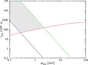
(a) Allowed region for $M_{1}=100$ GeV.

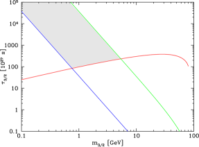
(b) Allowed region for $M_{1}=500$ GeV.

Figure 2: Allowed (shaded) region in the $m_{3/2}-\tau_{3/2}$ plane. The region above the nearly horizontal (red) line is allowed by the constraint in eq. (41). The region between the oblique lines is allowed by minimum (green) and maximum (blue) values of $|U_{\widetilde{\gamma}\nu}|^{2}$.

We stress that this analysis assumes that $m_{3/2}<m_{W}$. For a gravitino with a mass greater than the $Z$ boson mass the two-body decays $\widetilde{G}\rightarrow Z\nu$ and $\widetilde{G}\rightarrow W\ell$ will be kinematically allowed. As shown in ref. Ibarra:2007wg , the branching ratio of the decay $\widetilde{G}\rightarrow\gamma\nu$ becomes very small for a gravitino mass above $100$ GeV, and so the monochromatic line in the photon spectrum becomes less important. A more detailed analysis of the photon spectrum produced by the decay of the gravitino would be required in that case, which would need to include the fragmentation of the $W$ and $Z$ bosons in addition to the contribution from the 3-body decays.

VII Summary

It is explained how PSS in combination with RpV allows to generate the neutrino masses and mixings at the one loop level. Then it is investigated whether in this model the gravitino still is a good dark matter candidate. In order to do this the gravitino decay rates into two and three-body states are calculated. In the three-body decay corrections are found to previous calculations. Since for relatively small gravitino masses the decay is dominated by the two-body decay, the corrections in the three-body case do not affect the final result. Those rates allow to calculate the additional photon flux that is induced by the gravitino decay. Comparison of this photon flux with recent data from the Fermi LAT collaboration, allows to put restrictions on our model in the gravitino decay process.

Finally, combining the restrictions obtained in the neutrino sector with the restrictions in the gravitino dark matter sector of the same model, an upper limit on the gravitino mass $m_{3/2}<6$ GeV is found. The exact values of the maximal $m_{3/2}$ and the minimal $\tau_{3/2}$ in our model are given in table 3. One observes a relatively weak $M_{1}$ dependence.

$M_{1}$ [GeV]	$\tau_{3/2}$(min) [s]	$m_{3/2}$(max) [GeV]
$100$	$4.7\times 10^{28}$	$2.3$
$300$	$7.2\times 10^{28}$	$4.4$
$500$	$8.6\times 10^{28}$	$5.3$

Table 3: Minimal values of $\tau_{3/2}$ and maximal values of $m_{3/2}$ as a function of $M_{1}$.

It is interesting to note that most direct dark matter search experiments disfavor the typical heavy dark matter particle that appears in R-Parity conserving supersymmetric models Ahmed:2009zw ; Aprile:2011hi . The bound, however, is not even closely as tight for a light dark matter gravitino as it is found here. On the other hand, with the derived limit, the model turns out to be directly testable. For instance, if a relatively heavy dark matter particle is found with $m_{3/2}\gg 10$ GeV, one could immediately conclude that this model is ruled out. This feature of testability and the possibility of falsification can be seen as a strong advantage over many other models.

VIII Appendix: Three-body decays formulas

We label the five relevant diagrams with indices 1 to 5 as indicated in the text. For the photon and $Z$ mediated diagrams we define the invariant masses $s:=(k_{1}+k_{2})^{2}$, and $t:=(k_{1}+q)^{2}$, where $k_{1}$, $k_{2}$ and $q$ are the 4-momenta of the fermion, antifermion and neutrino, respectively. For the spin-averaged squared amplitudes and interferences we find (we define $m\equiv m_{3/2}$ for simplicity),

$$\langle|\mathcal{M}_{1}|^{2}\rangle=\frac{1}{4}\left(\frac{q_{f}^{2}|U_{\widetilde{\gamma}\nu_{i}}|^{2}}{16M_{P}^{2}}\right)\frac{1}{s^{2}}~{}T_{11},$$ (43)

$$\langle|\mathcal{M}_{2}|^{2}\rangle=\frac{1}{4}\left(\frac{g^{2}|U_{\widetilde{Z}\nu_{i}}|^{2}}{16c_{W}^{2}M_{P}^{2}}\right)\frac{1}{(s-m_{Z}^{2})^{2}+m_{Z}^{2}\Gamma_{Z}^{2}}~{}T_{22},$$ (44)

$$\langle|\mathcal{M}_{3}|^{2}\rangle=\frac{1}{4}\left(\frac{g^{4}\Lambda_{i}^{2}}{64\mu^{2}c_{W}^{4}M_{P}^{2}}\right)\frac{1}{(s-m_{Z}^{2})^{2}+m_{Z}^{2}\Gamma_{Z}^{2}}~{}{T}_{33},$$ (45)

$$2\Re\langle\mathcal{M}_{1}^{*}\mathcal{M}_{2}\rangle=\frac{2}{4}\left(\frac{gq_{f}U_{\widetilde{\gamma}\nu_{i}}U_{\widetilde{Z}\nu_{i}}}{16c_{W}M_{P}^{2}}\right)\frac{(s-m_{Z}^{2})}{s\left[(s-m_{Z}^{2})^{2}+m_{Z}^{2}\Gamma_{Z}^{2}\right]}~{}{T}_{12},$$ (46)

$$2\Re\langle\mathcal{M}_{1}^{*}\mathcal{M}_{3}\rangle=\frac{2}{4}\left(\frac{g^{2}q_{f}U_{\widetilde{\gamma}\nu_{i}}\Lambda_{i}}{32\mu c_{W}^{2}M_{P}^{2}}\right)\frac{(s-m_{Z}^{2})}{s\left[(s-m_{Z}^{2})^{2}+m_{Z}^{2}\Gamma_{Z}^{2}\right]}~{}{T}_{13},$$ (47)

$$2\Re\langle\mathcal{M}_{2}^{*}\mathcal{M}_{3}\rangle=\frac{2}{4}\left(\frac{g^{3}U_{\widetilde{Z}\nu_{i}}\Lambda_{i}}{32\mu c_{W}^{3}M_{P}^{2}}\right)\frac{1}{(s-m_{Z}^{2})^{2}+m_{Z}^{2}\Gamma_{Z}^{2}}~{}T_{23}.$$ (48)

For the $W$-mediated diagrams, we define $s$ and $t$ as above, with $k_{1}$, $k_{2}$ and $q$ the 4-momenta of the neutrino, antilepton and lepton, respectively. We find,

$$\langle|\mathcal{M}_{4}|^{2}\rangle=\frac{1}{4}\left(\frac{g^{2}|U_{\widetilde{W}\ell^{\prime}_{i}}|^{2}}{128M_{P}^{2}}\right)\frac{1}{(s-m_{W}^{2})^{2}+m_{W}^{2}\Gamma_{W}^{2}}~{}T_{44},$$ (49)

$$\langle|\mathcal{M}_{5}|^{2}\rangle=\frac{1}{4}\left(\frac{g^{4}\Lambda_{i}^{2}}{256\mu^{2}M_{P}^{2}}\right)\frac{1}{(s-m_{W}^{2})^{2}+m_{W}^{2}\Gamma_{W}^{2}}~{}{T}_{55},$$ (50)

$$2\Re\langle\mathcal{M}_{4}^{*}\mathcal{M}_{5}\rangle=\frac{2}{4}\left(\frac{g^{3}U_{\widetilde{W}\ell^{\prime}_{i}}\Lambda_{i}}{128\sqrt{2}\mu M_{P}^{2}}\right)\frac{1}{(s-m_{W}^{2})^{2}+m_{W}^{2}\Gamma_{W}^{2}}~{}T_{45}.$$ (51)

Finally, for the interference terms between these two groups of diagrams (when $f=\ell^{\prime}=\ell$), we define $s$ and $t$ as above, with $k_{1}$, $k_{2}$ and $q$ the 4-momenta of the lepton, antilepton and neutrino, respectively. We find,

$$2\Re\langle\mathcal{M}_{1}^{*}\mathcal{M}_{4}\rangle=\frac{2}{4}\left(\frac{gq_{f}U_{\widetilde{\gamma}\nu_{i}}U_{\widetilde{W}\ell_{i}}}{32\sqrt{2}M_{P}^{2}}\right)\frac{(m^{2}-(s+t)-m_{W}^{2})}{s\left[(m^{2}-(s+t)-m_{W}^{2})^{2}+m_{W}^{2}\Gamma_{W}^{2}\right]}~{}T_{14},$$ (52)

$$2\Re\langle\mathcal{M}_{2}^{*}\mathcal{M}_{4}\rangle=\frac{2}{4}\left(\frac{g^{2}U_{\widetilde{Z}\nu_{i}}U_{\widetilde{W}\ell_{i}}}{32\sqrt{2}c_{W}M_{P}^{2}}\right)\frac{(s-m_{Z}^{2})(m^{2}-(s+t)-m_{W}^{2})+m_{Z}m_{W}\Gamma_{Z}\Gamma_{W}}{\left[(s-m_{Z}^{2})^{2}+m_{Z}^{2}\Gamma_{Z}^{2}\right]\left[(m^{2}-(s+t)-m_{W}^{2})^{2}+m_{W}^{2}\Gamma_{W}^{2}\right]}~{}T_{24},$$ (53)

$$2\Re\langle\mathcal{M}_{3}^{*}\mathcal{M}_{4}\rangle=\frac{2}{4}\left(\frac{g^{3}U_{\widetilde{W}\ell_{i}}\Lambda_{i}}{64\sqrt{2}\mu c_{W}^{2}M_{P}^{2}}\right)\frac{(s-m_{Z}^{2})(m^{2}-(s+t)-m_{W}^{2})+m_{Z}m_{W}\Gamma_{Z}\Gamma_{W}}{\left[(s-m_{Z}^{2})^{2}+m_{Z}^{2}\Gamma_{Z}^{2}\right]\left[(m^{2}-(s+t)-m_{W}^{2})^{2}+m_{W}^{2}\Gamma_{W}^{2}\right]}~{}T_{34},$$ (54)

$$2\Re\langle\mathcal{M}_{1}^{*}\mathcal{M}_{5}\rangle=\frac{2}{4}\left(\frac{g^{2}q_{f}U_{\widetilde{\gamma}\nu_{i}}\Lambda_{i}}{64\mu M_{P}^{2}}\right)\frac{(m^{2}-(s+t)-m_{W}^{2})}{s\left[(m^{2}-(s+t)-m_{W}^{2})^{2}+m_{W}^{2}\Gamma_{W}^{2}\right]}~{}T_{15},$$ (55)

$$2\Re\langle\mathcal{M}_{2}^{*}\mathcal{M}_{5}\rangle=\frac{2}{4}\left(\frac{g^{3}U_{\widetilde{Z}\nu_{i}}\Lambda_{i}}{64\mu c_{W}M_{P}^{2}}\right)\frac{(s-m_{Z}^{2})(m^{2}-(s+t)-m_{W}^{2})+m_{Z}m_{W}\Gamma_{Z}\Gamma_{W}}{\left[(s-m_{Z}^{2})^{2}+m_{Z}^{2}\Gamma_{Z}^{2}\right]\left[(m^{2}+-(s+t)-m_{W}^{2})^{2}+m_{W}^{2}\Gamma_{W}^{2}\right]}~{}T_{25},$$ (56)

$$2\Re\langle\mathcal{M}_{3}^{*}\mathcal{M}_{5}\rangle=\frac{2}{4}\left(\frac{g^{4}\Lambda_{i}^{2}}{128\mu^{2}c_{W}^{2}M_{P}^{2}}\right)\frac{(s-m_{Z}^{2})(m^{2}-(s+t)-m_{W}^{2})+m_{Z}m_{W}\Gamma_{Z}\Gamma_{W}}{\left[(s-m_{Z}^{2})^{2}+m_{Z}^{2}\Gamma_{Z}^{2}\right]\left[(m^{2}-(s+t)-m_{W}^{2})^{2}+m_{W}^{2}\Gamma_{W}^{2}\right]}~{}T_{35}.$$ (57)

The total amplitude of the 3-body decays is given by the sum of all these terms, each being summed over all the relevant flavors and colors of the final states. The traces in equations (43) to (57) are given by,

$$\begin{split}T_{11}=&~{}\frac{64}{3m^{2}}s\Big{\{}3m^{6}-3m^{4}(s+2t)+m^{2}(s^{2}+8st+6t^{2})-s(s^{2}+2t(s+t))\Big{\}},\end{split}$$ (58)

$$\begin{split}T_{22}=&~{}\frac{64}{3m^{2}}(c_{V}^{2}+c_{A}^{2})s\Big{\{}3m^{6}-3m^{4}(s+2t)+m^{2}(s^{2}+6t^{2}+8st)-s(s^{2}+2t(s+t))\Big{\}},\end{split}$$ (59)

$$\begin{split}T_{33}=&~{}\frac{64}{3m^{2}}\Big{\{}(c_{V}^{2}+c_{A}^{2})(m^{2}-s)(m^{2}(2s+t)-t(s+t))-2c_{V}c_{A}m^{2}s(m^{2}-s-2t)\Big{\}},\end{split}$$ (60)

$$\begin{split}T_{12}=&~{}\frac{64}{3m^{2}}c_{V}s\Big{\{}3m^{6}-3m^{4}(s+2t)+m^{2}(s^{2}+8st+6t^{2})-s(s^{2}+2t(s+t))\Big{\}},\end{split}$$ (61)

$$\begin{split}T_{13}=&~{}\frac{32}{3m}s\Big{\{}c_{V}(3m^{4}-2m^{2}(s+t)-s^{2}+2st+2t^{2})-c_{A}(3m^{2}-s)(m^{2}-s-2t)\Big{\}},\end{split}$$ (62)

$$\begin{split}T_{23}=&~{}\frac{32}{3m}s\Big{\{}(c_{V}^{2}+c_{A}^{2})(3m^{4}-2m^{2}(s+t)-s^{2}+2t^{2}+2st)\\ &-2c_{V}c_{A}(3m^{4}-2m^{2}(2s+3t)+s^{2}+2st)\Big{\}},\end{split}$$ (63)

$$\begin{split}T_{44}=&~{}\frac{128}{3m^{2}}s\Big{\{}3m^{6}-3m^{4}(s+2t)+m^{2}(s^{2}+8st+6t^{2})-s(s^{2}+2st+2t^{2})\Big{\}},\end{split}$$ (64)

$$\begin{split}T_{55}=&~{}\frac{128}{3m^{2}}\Big{\{}m^{4}(3s+t)-m^{2}(s+t)(3s+t)+st(s+t)\Big{\}},\end{split}$$ (65)

$$\begin{split}T_{45}=&~{}\frac{128}{3m}s\Big{\{}3m^{4}-m^{2}(3s+4t)+t(2s+t)\Big{\}},\end{split}$$ (66)

$$\begin{split}T_{14}=&~{}\frac{64}{3m^{2}}s\Big{\{}3m^{6}-m^{4}(3s+7t)+m^{2}t(4s+5t)-t^{2}(s+t)\Big{\}},\end{split}$$ (67)

$$\begin{split}T_{24}=&~{}\frac{64}{3m^{2}}(c_{V}-c_{A})s\Big{\{}3m^{6}-m^{4}(3s+7t)+m^{2}t(4s+5t)-t^{2}(s+t)\Big{\}},\end{split}$$ (68)

$$\begin{split}T_{34}=&~{}\frac{64}{3m^{2}}(c_{V}-c_{A})\Big{\{}m^{5}(3s+t)-m^{3}(3s^{2}+6st+2t^{2})+mt(s+t)(2s+t)\Big{\}},\end{split}$$ (69)

$$\begin{split}T_{15}=&~{}\frac{64}{3m}s\Big{\{}3m^{4}-m^{2}(3s+4t)+t(2s+t)\Big{\}},\end{split}$$ (70)

$$\begin{split}T_{25}=&~{}\frac{64}{3m}(c_{V}-c_{A})s\Big{\{}3m^{4}-m^{2}(3s+4t)+t(2s+t)\Big{\}},\end{split}$$ (71)

$$\begin{split}T_{35}=&~{}\frac{64}{3m^{2}}(c_{V}-c_{A})\Big{\{}(m^{2}-s)(m^{2}s+(m^{2}-t)(s+t))+m^{2}s(m^{2}-s-2t)\Big{\}}.\end{split}$$ (72)

Finally those amplitudes are applied to the golden rule for decays in order to obtain the partial and total decay rate for each process $\tilde{G}\rightarrow 2+3+4$

$$d\Gamma=|{\mathcal{M}}|^{2}\frac{S}{2m_{3/2}}\left[\frac{d^{3}p_{2}}{(2\pi)^{3}2E_{2}}\frac{d^{3}p_{3}}{(2\pi)^{3}2E_{3}}\frac{d^{3}p_{4}}{(2\pi)^{3}2E_{4}}\right](2\pi)^{4}\delta^{4}(p_{1}-p_{2}-p_{3}-p_{4})\quad.$$ (73)

References

- (1) N. Arkani-Hamed and S. Dimopoulos, JHEP 0506, 073 (2005) [arXiv:hep-th/0405159]; G. F. Giudice and A. Romanino, Nucl. Phys. B 699, 65 (2004) [Erratum-ibid. B 706, 65 (2005)] [arXiv:hep-ph/0406088].
- (2) G. Aad et al. [The ATLAS Collaboration], arXiv:0901.0512 [hep-ex]; P. de Jong, AIP Conf. Proc. 1078, 21 (2009) [arXiv:0809.3708 [hep-ex]].
- (3) R. Barbier et al., Phys. Rept. 420, 1 (2005) [arXiv:hep-ph/0406039].
- (4) M. Nowakowski and A. Pilaftsis, Nucl. Phys. B 461, 19 (1996) [arXiv:hep-ph/9508271]; R. Hempfling, Nucl. Phys. B 478, 3 (1996) [arXiv:hep-ph/9511288].
- (5) M. Hirsch, M. A. Diaz, W. Porod, J. C. Romao and J. W. F. Valle, Phys. Rev. D 62, 113008 (2000) [Erratum-ibid. D 65, 119901 (2002)] [arXiv:hep-ph/0004115].
- (6) E. J. Chun and S. C. Park, JHEP 0501, 009 (2005) [arXiv:hep-ph/0410242]; S. Davidson and M. Losada, Phys. Rev. D 65, 075025 (2002) [arXiv:hep-ph/0010325]; S. Davidson and M. Losada, JHEP 0005, 021 (2000) [arXiv:hep-ph/0005080]; Y. Grossman and S. Rakshit, Phys. Rev. D 69, 093002 (2004) [arXiv:hep-ph/0311310].
- (7) M. A. Diaz, P. Fileviez Perez and C. Mora, Phys. Rev. D 79, 013005 (2009) [arXiv:hep-ph/0605285].
- (8) M. A. Diaz, B. Koch, B. Panes, Phys. Rev. D79, 113009 (2009). [arXiv:0902.1720 [hep-ph]].
- (9) R. Sundrum, JHEP 1101, 062 (2011). [arXiv:0909.5430 [hep-th]].
- (10) M. A. Diaz, F. Garay and B. Koch, Phys. Rev. D 80, 113005 (2009) [arXiv:0910.2987 [hep-ph]].
- (11) M. Grefe, “Neutrino signals from gravitino dark matter with broken R-parity,” DESY-THESIS-2008-043; L. Covi, arXiv:1003.3819 [hep-ph]; W. Buchmuller, AIP Conf. Proc. 1200, 155 (2010) [arXiv:0910.1870 [hep-ph]].
- (12) F. Wang, W. Wang and J. M. Yang, Phys. Rev. D 72, 077701 (2005) [arXiv:hep-ph/0507172].
- (13) F. Takayama and M. Yamaguchi, Phys. Lett. B 485, 388 (2000) [arXiv:hep-ph/0005214].
- (14) K. Ishiwata, S. Matsumoto and T. Moroi, Phys. Rev. D 78, 063505 (2008) [arXiv:0805.1133 [hep-ph]].
- (15) A. Ibarra and D. Tran, Phys. Rev. Lett. 100, 061301 (2008) [arXiv:0709.4593 [astro-ph]].
- (16) H. Yuksel and M. D. Kistler, Phys. Rev. D 78, 023502 (2008) [arXiv:0711.2906 [astro-ph]].
- (17) K. Y. Choi, D. E. Lopez-Fogliani, C. Munoz and R. R. de Austri, JCAP 1003, 028 (2010) [arXiv:0906.3681 [hep-ph]].
- (18) W. Buchmuller, L. Covi, K. Hamaguchi, A. Ibarra and T. Yanagida, JHEP 0703, 037 (2007) [arXiv:hep-ph/0702184].
- (19) G. Bertone, W. Buchmuller, L. Covi and A. Ibarra, JCAP 0711, 003 (2007) [arXiv:0709.2299 [astro-ph]].
- (20) K. Y. Choi, D. Restrepo, C. E. Yaguna and O. Zapata, JCAP 1010, 033 (2010) [arXiv:1007.1728 [hep-ph]].
- (21) K. Y. Choi and C. E. Yaguna, Phys. Rev. D 82, 015008 (2010) [arXiv:1003.3401 [hep-ph]].
- (22) A. A. Abdo et al. [The Fermi LAT collaboration], arXiv:1003.0895 [astro-ph.CO].
- (23) A. A. Abdo et al. [The Fermi LAT collaboration], Phys. Rev. Lett. 104, 101101 (2010) [arXiv:1002.3603 [astro-ph.HE]].
- (24) W. B. Atwood et al. [The Fermi LAT collaboration], Astrophys. J. 697, 1071 (2009) [arXiv:0902.1089 [astro-ph.IM]].
- (25) A. A. Abdo et al. [The Fermi LAT collaboration], Phys. Rev. Lett. 103, 251101 (2009) [arXiv:0912.0973 [astro-ph.HE]].
- (26) A. A. Abdo et al. [The Fermi LAT collaboration], Phys. Rev. Lett. 104, 091302 (2010) [arXiv:1001.4836 [astro-ph.HE]].
- (27) Z. Ahmed et al. [The CDMS-II Collaboration], Science 327, 1619 (2010) [arXiv:0912.3592 [astro-ph.CO]].
- (28) E. Aprile et al. [XENON100 Collaboration], arXiv:1104.2549 [astro-ph.CO].
- (29) B. Bajc, T. Enkhbat, D. K. Ghosh, G. Senjanovic and Y. Zhang, JHEP 1005, 048 (2010) [arXiv:1002.3631 [hep-ph]].
- (30) S. L. Chen, R. N. Mohapatra, S. Nussinov and Y. Zhang, Phys. Lett. B 677, 311 (2009) [arXiv:0903.2562 [hep-ph]].
- (31) M. Y. Khlopov and A. D. Linde, Phys. Lett. B 138, 265 (1984).
- (32) I. V. Falomkin, G. B. Pontecorvo, M. G. Sapozhnikov, M. Y. Khlopov, F. Balestra and G. Piragino, Nuovo Cim. A 79, 193 (1984) [Yad. Fiz. 39, 990 (1984)].
- (33) M. Y. Khlopov, A. Barrau and J. Grain, Class. Quant. Grav. 23, 1875 (2006) [arXiv:astro-ph/0406621].
- (34) N. Arkani-Hamed, S. Dimopoulos, G. F. Giudice, A. Romanino, Nucl. Phys. B709, 3-46 (2005). [arXiv:hep-ph/0409232 [hep-ph]].
- (35) M. Drees, [hep-ph/0501106].
- (36) B. C. Allanach, A. Dedes, H. K. Dreiner, Phys. Rev. D69, 115002 (2004). [hep-ph/0309196].
- (37) P. Fileviez Perez, S. Spinner, Phys. Rev. D83, 035004 (2011). [arXiv:1005.4930 [hep-ph]].
- (38) J. F. Navarro, C. S. Frenk and S. D. M. White, Astrophys. J. 462, 563 (1996) [arXiv:astro-ph/9508025].
- (39) W. Buchmuller, A. Ibarra, T. Shindou, F. Takayama and D. Tran, JCAP 0909, 021 (2009) [arXiv:0906.1187 [hep-ph]].
- (40) http://www-glast.slac.stanford.edu/software/IS/glast_lat_performance.htm
- (41) M. Maltoni, T. Schwetz, M. A. Tortola and J. W. F. Valle, New J. Phys. 6, 122 (2004) [arXiv:hep-ph/0405172].