A fast and reliable method for the calculation of band structure of solids with hybrid functionals

Abstract

A simple approximation within the framework of the hybrid methods for the calculation of the electronic structure of solids is presented. By considering only the diagonal elements of the perturbation operator (Hartree-Fock exchange minus semilocal exchange) calculated in the basis of the semilocal orbitals, the computational time is drastically reduced, while keeping very well in most studied cases the accuracy of the results obtained with hybrid functionals when applied without any approximations.

Quantum calculations for solids are commonly done with the local density approximation (LDA) or the generalized gradient approximation (GGA) of density-functional theory (DFT).HohenbergPR64 ; KohnPR65 While the properties calculated using the total energy (e.g., lattice constant) are fairly well described by LDA or GGA, the electronic band structure can not be described correctly in many cases. For instance, it is well known that the semilocal approximations (LDA and GGA) lead to unoccupied states in semiconductors and insulators which are too low in energy, and hence, to too small band gap with respect to experiment (see, e.g., Ref. StadelePRL97, ). More advanced theories can provide more accurate band structures. StadelePRL97 ; BechstedtPSSB09 ; AnisimovPRB91 ; BylanderPRB90 ; CoraSB04 ; TranPRL09 The best known are the $GW$ approximation to the self energy $\Sigma_{\text{xc}}$ within the many-body perturbation theory (Ref. HedinPR65, ) and the hybrid functionals BeckeJCP93a ; BeckeJCP93b which consist of a mixing of semilocal and Hartree-Fock (i.e., exact) exchange.

The $GW$ method represents the state-of-the-art,BechstedtPSSB09 and leads very often to very accurate results in particular if it is applied self-consistently FaleevPRL04 ; BrunevalPRL06 ; ShishkinPRL07 and with vertex corrections. ShishkinPRL07 However, due to the huge computational effort required by a $GW$ calculation, most of the $GW$ results from the literature were obtained non-self-consistently (i.e., one-shot $G_{0}W_{0}$). Within the $G_{0}W_{0}$ method, the quasiparticle energies $\epsilon_{n\textbf{k}}^{G_{0}W_{0}}$ are obtained as solutions of the nonlinear equation

$$\epsilon_{n\textbf{k}}^{G_{0}W_{0}}=\epsilon_{n\textbf{k}}^{\text{SL}}+\langle\psi_{n\textbf{k}}^{\text{SL}}|\Sigma_{\text{xc}}(\epsilon_{n\textbf{k}}^{G_{0}W_{0}})-v_{\text{xc}}^{\text{SL}}|\psi_{n\textbf{k}}^{\text{SL}}\rangle,$$ (1)

where $\psi_{n\textbf{k}}^{\text{SL}}$ and $\epsilon_{n\textbf{k}}^{\text{SL}}$ are the orbitals and the corresponding energies obtained from a previous DFT calculation with a semilocal (SL) functional $E_{\text{xc}}^{\text{SL}}$ [in Eq. (1), $v_{\text{xc}}^{\text{SL}}=\delta E_{\text{xc}}^{\text{SL}}/\delta\rho$]. The nondiagonal terms of the matrix of $\Sigma_{\text{xc}}-v_{\text{xc}}^{\text{SL}}$ are neglected.HedinIJQC95 The quasiparticle energies $\epsilon_{n\textbf{k}}^{G_{0}W_{0}}$ are most of the time close to experiment, but there are known cases (e.g., NiOvanSchilfgaardePRB06 ) were self-consistency is really needed. Beside the heavy cost of a $GW$ calculation ($G_{0}W_{0}$ can still be considered as a very expensive method), a drawback is that the convergence of the results with respect to the number of unoccupied states can be extremely slow as, for example, for ZnO.ShihPRL10 ; FriedrichPRB11

The hybrid functionals are becoming more and more popular for solids (see, e.g., Ref. CoraSB04, ). On average, the accuracy of the electronic band structure they provide is quite similar to $G_{0}W_{0}$. In hybrid functionals, a fraction $\alpha_{\text{x}}$ of semilocal exchange is replaced by the Hartree-Fock (HF) exchange:

$$E_{\text{xc}}^{\text{hybrid}}=E_{\text{xc}}^{\text{SL}}+\alpha_{\text{x}}\left(E_{\text{x}}^{\text{HF}}-E_{\text{x}}^{\text{SL}}\right).$$ (2)

The value of $\alpha_{\text{x}}$ which leads to the best agreement with experiment depends on (a) the system under study, (b) the considered property, and (c) the underlying semilocal functional $E_{\text{xc}}^{\text{SL}}$. Most of the time, the value of $\alpha_{\text{x}}$ lies in the range 0$-$0.5. Among the best known hybrid functionals, there is the so-called PBE0 ErnzerhofJCP99 ; AdamoJCP99 (the functional considered in the present work), where the semilocal functional in Eq. (2) is the GGA of Perdew, Burke, and ErnzerhofPerdewPRL96 (PBE) and the amount $\alpha_{\text{x}}$ of Hartree-Fock exchange is set to 0.25 (Ref. PerdewJCP96, ). Another way of constructing hybrid functionals consists of replacing only the short-range part of the semilocal exchange by short-range Hartree-Fock as proposed in Ref. HeydJCP03, for the HSE functional (also based on PBE), where the short- and long-range parts of exchange are defined by splitting the Coulomb operator with the error function. Not considering the long-range Hartree-Fock exchange avoids technical problems and makes the calculations faster. Note that the idea of screening the Hartree-Fock exchange was already used by Bylander and Kleinman for their screened-exchange LDA functional (sX-LDA), BylanderPRB90 which can be considered as a hybrid functional with 100% ($\alpha_{\text{x}}=1$) of short-range Hartree-Fock exchange (see Ref. ClarkPSSB11, for recent sX-LDA calculations). However, even without long-range Hartree-Fock, the use of hybrid functionals for solids leads to calculations which are one or two orders of magnitude more expensive than with semilocal functionals. The tendency of the PBE0 functional is to overestimate small ($<3$ eV) band gaps and to underestimate large ($>10$ eV) band gaps (see, e.g., Ref. MarquesPRB11, ), and due to the neglect of the long-range Hartree-Fock in HSE, the HSE band gaps are smaller than the PBE0 band gaps.HeydJCP05 ; PaierJCP06 ; MarquesPRB11 Note that in Ref. MarquesPRB11, it was shown that the performance of PBE0 and HSE could be improved by making the fraction $\alpha_{\text{x}}$ of Hartree-Fock exchange dependent on either the average of $\left|\nabla\rho\right|/\rho$ in the unit cell (as done in Ref. TranPRL09, for the modified Becke-Johnson potentialBeckeJCP06 ) or the static dielectric constant.

In this work, a fast way of getting the energies of orbitals from hybrid functionals is proposed. In Ref. TranPRB11, , the implementation of hybrid functionals (screened and unscreened) into the WIEN2k code, WIEN2k which is based on the full-potential linearized augmented plane-wave plus local orbitals method AndersenPRB75 ; SjostedtSSC00 to solve the Kohn-Sham equations, was reported. The Hartree-Fock method was implemented following the method of Massidda, Posternak, and Baldereschi,MassiddaPRB93 which is based on the pseudocharge method to solve the Poisson equation.WeinertJMP81

The calculation of the matrix of the nonlocal Hartree-Fock operator $\hat{v}_{\text{x}}^{\text{HF}}$ is done in a second variational procedure, i.e., the operator $\alpha_{\text{x}}\left(\hat{v}_{\text{x}}^{\text{HF}}-v_{\text{x}}^{\text{SL}}\right)$ is considered as a perturbation and the semilocal orbitals are used as basis functions:

$$\langle\psi_{n\mathbf{k}}^{\text{SL}}|\alpha_{\text{x}}\left(\hat{v}_{\text{x}}^{\text{HF}}-v_{\text{x}}^{\text{SL}}\right)|\psi_{n^{\prime}\mathbf{k}}^{\text{SL}}\rangle.$$ (3)

The second variational procedure, which was also adopted for the implementation of the Hartree-Fock equations in other LAPW codes MassiddaPRB93 ; AsahiPRB99 ; BetzingerPRB10 leads to cheaper calculations, since in practice the number of orbitals $\psi_{n\mathbf{k}}^{\text{SL}}$ which are used for the construction of Eq. (3) can be chosen to be much smaller than the number of LAPW basis functions. Since the shape of the orbitals obtained from the semilocal and hybrid functionals can be expected to be rather similar, the most important matrix elements of Eq. (3) are the diagonal ones. This leads to the simple proposition which consists of calculating the orbital energies from hybrid functional the following way:

$$\epsilon_{n\textbf{k}}^{\text{hybrid}}=\epsilon_{n\textbf{k}}^{\text{SL}}+\langle\psi_{n\mathbf{k}}^{\text{SL}}|\alpha_{\text{x}}\left(\hat{v}_{\text{x}}^{\text{HF}}-v_{\text{x}}^{\text{SL}}\right)|\psi_{n\mathbf{k}}^{\text{SL}}\rangle,$$ (4)

i.e., the nondiagonal terms are neglected, similarly as done in Eq. (1) for the $G_{0}W_{0}$ method.HedinIJQC95 Obviously, within this approximation the orbitals are not updated since the matrix of the operator $\alpha_{\text{x}}\left(\hat{v}_{\text{x}}^{\text{HF}}-v_{\text{x}}^{\text{SL}}\right)$ [Eq. (3)] is diagonal, which means that the $\psi_{n\mathbf{k}}^{\text{SL}}$s are already the eigenvectors. In the following, the results obtained with Eq. (4) will be named PBE0₀ (i.e., one-shot PBE0) in analogy with $G_{0}W_{0}$. Compared to a self-consistent calculation, using Eq. (4) leads to calculations of the band structure which are at least two orders of magnitude faster (neglect of the nondiagonal terms and only one iteration). Naturally, the PBE orbitals were used as the semilocal orbitals in Eq. (4). Actually, Eq. (4) is also very closely related to the way the exchange part of the derivative discontinuity is calculated:

$$\Delta_{\text{x}}=\langle\psi_{n^{\prime}\mathbf{k}^{\prime}}|\hat{v}_{\text{x}}^{\text{HF}}-v_{\text{x}}^{\text{EXX}}|\psi_{n^{\prime}\mathbf{k}^{\prime}}\rangle-\langle\psi_{n\mathbf{k}}|\hat{v}_{\text{x}}^{\text{HF}}-v_{\text{x}}^{\text{EXX}}|\psi_{n\mathbf{k}}\rangle,$$ (5)

where $\psi_{n\mathbf{k}}$ and $\psi_{n^{\prime}\mathbf{k}^{\prime}}$ are the orbitals at the valence band maximum and conduction band minimum, respectively, and $v_{\text{x}}^{\text{EXX}}$ is the multiplicative exact exchange (EXX) potential obtained with the optimized effective potential method [see Ref. StadelePRL97, for more discussion on Eq. (5)].

In order to test the accuracy of Eq. (4) for the calculation of the orbital energies, we have considered the following semiconductors and insulators (the structure and cubic lattice constant are given in parenthesis): Ar (fcc, 5.260 Å), C (diamond, 3.567 Å), Si (diamond, 5.430 Å), GaAs (zinc blende, 5.648 Å), MgO (rocksalt, 4.207 Å), NaCl (rocksalt, 5.595 Å), Cu₂O ($Pn\overline{3}m$, 4.27 Å), MnO ($Fm\overline{3}m$, 4.445 Å), and NiO ($Fm\overline{3}m$, 4.171 Å). The unit cell of Cu₂O contains six atoms. Formally, Cu has a valency of $+1$ and therefore the Cu-$3d$ shell is full, which means that the correlation effects in the Cu-$3d$ shell should not play an important role as it is the case for CuO.GhijsenPRB08 MnO and NiO have a cubic symmetry, but by taking into account the antiferromagnetic phase (along the [111] direction of the cubic cell), the symmetry is reduced to a rhombohedral one (four atoms in the unit cell). MnO and NiO are two of the most studied Mott insulators, for which the semilocal functionals are very inaccurate due to the strongly localized character of the $3d$ electrons.TerakuraPRB84 Detailed descriptions of the structures of Cu₂O and MnO/NiO can be found in Refs. MarksteinerZPB86, and CococcioniPRB05, , respectively.

Table 1: Transition energies (in eV) obtained with the PBE, PBE0, and PBE0₀ methods. The experimental value for Cu₂O is from Ref. BaumeisterPR61, . See Table I of Ref. BetzingerPRB10, for the other solids.

Solid	Transition	PBE	PBE0	PBE00	Expt.
Ar	$\Gamma\rightarrow\Gamma$	8.69	11.09	11.11	14.2
C	$\Gamma\rightarrow\Gamma$	5.59	7.69	7.64	7.3
	$\Gamma\rightarrow X$	4.76	6.64	6.59
	$\Gamma\rightarrow L$	8.46	10.76	10.73
Si	$\Gamma\rightarrow\Gamma$	2.56	3.95	3.90	3.4
	$\Gamma\rightarrow X$	0.71	1.91	1.87
	$\Gamma\rightarrow L$	1.53	2.86	2.80	2.4
GaAs	$\Gamma\rightarrow\Gamma$	0.53	1.99	1.87	1.63
	$\Gamma\rightarrow X$	1.46	2.66	2.65	2.18, 2.01
	$\Gamma\rightarrow L$	1.01	2.35	2.29	1.84, 1.85
MgO	$\Gamma\rightarrow\Gamma$	4.79	7.23	7.23	7.7
	$\Gamma\rightarrow X$	9.16	11.58	11.65
	$\Gamma\rightarrow L$	7.95	10.43	10.48
NaCl	$\Gamma\rightarrow\Gamma$	5.22	7.29	7.28	8.5
	$\Gamma\rightarrow X$	7.59	9.80	9.80
	$\Gamma\rightarrow L$	7.33	9.40	9.40
Cu2O	$\Gamma\rightarrow\Gamma$	0.53	2.77	2.68	2.17
MnO	$\Gamma\rightarrow\Gamma$	1.47	4.23	4.04
NiO	$\Gamma\rightarrow\Gamma$	2.41	6.07	5.91

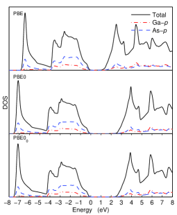
Figure 1: (Color online) Density of states of GaAs calculated with the PBE, PBE0, and PBE0₀ methods. The Fermi energy is set at zero.

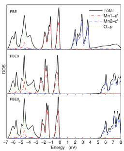
Figure 2: (Color online) Density of states of one spin component of MnO calculated with the PBE, PBE0, and PBE0₀ methods. The Fermi energy is set at zero.

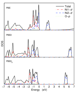
Figure 3: (Color online) Density of states of one spin component of NiO calculated with the PBE, PBE0, and PBE0₀ methods. The Fermi energy is set at zero.

The calculated transition energies, along with experimental values, are shown in Table 1. As expected, the PBE transition energies are by far too small compared to the experiment, while the PBE0 values are much larger and closer to the experiment. However, as already mentioned above, PBE0 overestimates small transition energies (e.g., GaAs) and underestimates large transition energies (e.g., Ar). Actually, the important observation of the present work is that the PBE0 transition energies calculated with the approximation given by Eq. (4) (PBE0₀ in Table 1) are very similar to the self-consistent PBE0 results. Indeed, the largest difference is for MnO ($\sim 0.2$ eV), which, anyway, represents less than 10% of the difference between PBE (1.47 eV) and PBE0 (4.23 eV). For the $\Gamma\rightarrow\Gamma$ transition in GaAs and Cu₂O, the difference between PBE0 and PBE0₀ is $\sim 0.1$ eV and less than 0.1 eV in all other cases. In the case of MgO and NaCl, the accuracy of Eq. (4) is impressive.

Figures 1, 2, and 3 show the density of states (DOS) of GaAs, MnO, and NiO, respectively. In the case of GaAs, the PBE0 and PBE0₀ DOSs are indistinguishable, which can be explained by the fact that already the PBE and PBE0 DOSs are very similar and differ only by the shift of the unoccupied bands. For MnO as well, the agreement between PBE0 and PBE0₀ is very good, albeit small differences can be seen. In the case of NiO (the most difficult case considered in this work), more visible differences between PBE0 and PBE0₀ can be observed. For instance, the PBE0₀ DOS in the energy range $-7$ and $-3$ eV looks intermediate between the PBE and PBE0 DOSs. There is less O-$p$ states in the latter case. Also, the unoccupied Ni-$d$ peaks are higher in energy by $\sim 0.8$ eV with PBE0 than with PBE0₀.

In Refs. vanSchilfgaardePRB06, and FaleevPRL04, , band gaps of 1.1 and 4.8 eV for NiO calculated with non-self-consistent [Eq. (1)] and self-consistent $GW$ calculations, respectively, were reported. The importance of self-consistency in this case is rather extreme. Such a huge difference is not observed for NiO with hybrid functionals when using Eq. (4) instead of doing a self-consistent PBE0 calculation. The explanation lies in the fact that in the case of Eq. (4), only the semilocal orbitals are used for the construction of the nonlocal Hartree-Fock operator $\hat{v}_{\text{x}}^{\text{HF}}$, while for $G_{0}W_{0}$ [Eq. (1)] both the orbitals and their energies are used for the calculation of the self-energy $\Sigma_{\text{xc}}$. In the case of Cu₂O it was shown in Ref. BrunevalPRL06, , that with respect to non-self-consistent $G_{0}W_{0}$, updating only the orbital energies in $\Sigma_{\text{xc}}$ already increases the band by 0.46 eV (from 1.34 to 1.80 eV), while updating also the orbitals increases further the band gap, but by a much smaller value (0.17 eV). Other such examples can be found in Ref. ShishkinPRB07, . However, the effect of self-consistency in the $GW$ method can be reduced if the input orbitals and energies are calculated from the hybrid (see Ref. BechstedtPSSB09, ) or $\text{LDA}+U$ (see Ref. JiangPRB10, ) methods.

In summary, it has been shown that for calculations with hybrid functionals, neglecting the nondiagonal terms in the construction of the Hartree-Fock Hamiltonian (within the second variational procedure) leads to a very good approximation. By doing so, the orbital energies [Eq. (4)] are very close to the energies obtained from a self-consistent calculation done without any approximations. Several types of semiconductors and insulators, including the more difficult cases of antiferromagnetic MnO and NiO, have been considered and the accuracy of the approximation has been shown to be (very) good in most cases. For NiO, the results are less impressive than in the other cases. The approximation leads to calculations of the band structure of solids with hybrid functionals which are at least two orders of magnitude faster than the self-consistent calculations. This approximation allows the calculation of the electronic band structure of solids with hybrid functionals on much larger systems.

- (1) P. Hohenberg and W. Kohn, Phys. Rev. 136, B864 (1964).
- (2) W. Kohn and L. J. Sham, Phys. Rev. 140, A1133 (1965).
- (3) M. Städele, J. A. Majewski, P. Vogl, and A. Görling, Phys. Rev. Lett. 79, 2089 (1997).
- (4) F. Bechstedt, F. Fuchs, and G. Kresse, Phys. Status Solidi B 246, 1877 (2009).
- (5) V. I. Anisimov, J. Zaanen, and O. K. Andersen, Phys. Rev. B 44, 943 (1991).
- (6) D. M. Bylander and L. Kleinman, Phys. Rev. B 41, 7868 (1990).
- (7) F. Corà, M. Alfredsson, G. Mallia, D. S. Middlemiss, W. C. Mackrodt, R. Dovesi, and R. Orlando, Struct. Bonding (Berlin) 113, 171 (2004).
- (8) F. Tran and P. Blaha, Phys. Rev. Lett. 102, 226401 (2009).
- (9) L. Hedin, Phys. Rev. 139, A796 (1965).
- (10) A. D. Becke, J. Chem. Phys. 98, 1372 (1993).
- (11) A. D. Becke, J. Chem. Phys. 98, 5648 (1993).
- (12) S. V. Faleev, M. van Schilfgaarde, and T. Kotani, Phys. Rev. Lett. 93, 126406 (2004).
- (13) F. Bruneval, N. Vast, L. Reining, M. Izquierdo, F. Sirotti, and N. Barrett, Phys. Rev. Lett. 97, 267601 (2006).
- (14) M. Shishkin, M. Marsman, and G. Kresse, Phys. Rev. Lett. 99, 246403 (2007).
- (15) L. Hedin, Int. J. Quantum Chem. 56, 445 (1995).
- (16) M. van Schilfgaarde, T. Kotani, and S. V. Faleev, Phys. Rev. B 74, 245125 (2006).
- (17) B.-C. Shih, Y. Xue, P. Zhang, M. L. Cohen, and S. G. Louie, Phys. Rev. Lett. 105, 146401 (2010).
- (18) C. Friedrich, M. C. Müller, and S. Blügel, Phys. Rev. B 83, 081101(R) (2011).
- (19) M. Ernzerhof and G. E. Scuseria, J. Chem. Phys. 110, 5029 (1999).
- (20) C. Adamo and V. Barone, J. Chem. Phys. 110, 6158 (1999).
- (21) J. P. Perdew, K. Burke, and M. Ernzerhof, Phys. Rev. Lett. 77, 3865 (1996); 78, 1396 (1997).
- (22) J. P. Perdew, M. Ernzerhof, and K. Burke, J. Chem. Phys. 105, 9982 (1996).
- (23) J. Heyd, G. E. Scuseria, and M. Ernzerhof, J. Chem. Phys. 118, 8207 (2003); 124, 219906 (2006).
- (24) S. J. Clark and J. Robertson, Phys. Status Solidi B 248, 537 (2011).
- (25) M. A. L. Marques, J. Vidal, M. J. T. Oliveira, L. Reining, and S. Botti, Phys. Rev. B 83, 035119 (2011).
- (26) J. Heyd, J. E. Peralta, G. E. Scuseria, and R. L. Martin, J. Chem. Phys. 123, 174101 (2005).
- (27) J. Paier, M. Marsman, K. Hummer, G. Kresse, I. C. Gerber, and J. G. Ángyán, J. Chem. Phys. 124, 154709 (2006); 125, 249901 (2006).
- (28) A. D. Becke and E. R. Johnson, J. Chem. Phys. 124, 221101 (2006).
- (29) F. Tran and P. Blaha, Phys. Rev. B 83, 235118 (2011).
- (30) P. Blaha, K. Schwarz, G. K. H. Madsen, D. Kvasnicka, and J. Luitz, wien2k: An Augmented Plane Wave plus Local Orbitals Program for Calculating Crystal Properties, edited by K. Schwarz (Vienna University of Technology, Austria, 2001).
- (31) O. K. Andersen, Phys. Rev. B 12, 3060 (1975).
- (32) E. Sjöstedt, L. Nordström, and D. J. Singh, Solid State Commun. 114, 15 (2000).
- (33) S. Massidda, M. Posternak, and A. Baldereschi, Phys. Rev. B 48, 5058 (1993).
- (34) M. Weinert, J. Math. Phys. 22, 2433 (1981).
- (35) R. Asahi, W. Mannstadt, and A. J. Freeman, Phys. Rev. B 59, 7486 (1999).
- (36) M. Betzinger, C. Friedrich, and S. Blügel, Phys. Rev. B 81, 195117 (2010).
- (37) J. Ghijsen, L. H. Tjeng, J. van Elp, H. Eskes, J. Westerink, G. A. Sawatzky, and M. T. Czyzyk, Phys. Rev. B 38, 11322 (1988).
- (38) K. Terakura, T. Oguchi, A. R. Williams, and J. Kübler, Phys. Rev. B 30, 4734 (1984).
- (39) P. Marksteiner, P. Blaha, and K. Schwarz, Z. Phys. B: Condens. Matter 64, 119 (1986).
- (40) M. Cococcioni and S. de Gironcoli, Phys. Rev. B 71, 035105 (2005).
- (41) P. W. Baumeister, Phys. Rev. 121, 359 (1961).
- (42) M. Shishkin and G. Kresse, Phys. Rev. B 75, 235102 (2007).
- (43) H. Jiang, R. I. Gomez-Abal, P. Rinke, and M. Scheffler, Phys. Rev. B 82, 045108 (2010).