Approach to equilibrium of diffusion in a logarithmic potential

Abstract

The late-time distribution function $P(x,t)$ of a particle diffusing in a one-dimensional logarithmic potential is calculated for arbitrary initial conditions. We find a scaling solution with three surprising features: (i) the solution is given by two distinct scaling forms, corresponding to a diffusive ($x\sim t^{1/2}$) and a subdiffusive ($x\sim t^{\gamma}$ with a given $\gamma<1/2$) length scale, respectively, (ii) the overall scaling function is selected by the initial condition, and (iii) depending on the tail of the initial condition, the scaling exponent which characterizes the scaling function is found to exhibit a transition from a continuously varying to a fixed value.

I Introduction

There exist many physical systems whose temporal evolution is described by a diffusion process in a one-dimensional logarithmic potential. Examples include the denaturation process of DNA molecules Bar et al. (2009) and the temporal evolution of the momentum distribution of cold atoms trapped in an optical lattice Castin et al. (1991); Marksteiner et al. (1996); Lutz (2004). Effective logarithmic potentials also appear, for example, in models of real-space condensation such as the zero-range process Evans and Hanney (2005); Godrèche and Luck (2001); Levine et al. (2005), relaxation to equilibrium of long-range interacting gases Bouchet and Dauxois (2005); Campa et al. (2009), dynamics of the two-dimensional $XY$ model below the Kosterlitz-Thouless transition Bray (2000), the ABBM model for Barkhausen noise Durin and Zapperi (2006), and dynamics of sleep-wake transitions during a night’s sleep Lo et al. (2002).

The Fokker-Planck equation corresponding to diffusion in a one-dimensional potential is

$$\frac{\partial P(x,t)}{\partial t}=\frac{\partial}{\partial x}\Bigl{[}V^{\prime}(x)P(x,t)+\frac{\partial P(x,t)}{\partial x}\Bigr{]},$$ (1)

where $P(x,t)$ is the probability distribution. We consider potentials which increase logarithmically at large $x$,

$$V(|x|\gg 1)\sim b\log(|x|),$$ (2)

and are regular at $x=0$. For simplicity, we have taken in these equations the diffusion constant and the temperature to be equal to 1. Here we consider the case $b>1$, for which the system evolves into a stationary state given by the normalizable Boltzmann distribution

$$P^{*}(x)=\frac{1}{Z}e^{-V(x)}\sim\frac{1}{Z}x^{-b}$$ (3)

where $Z=\int e^{-V(x)}dx$ is the normalization constant. For some applications the variable $x$ is by definition non-negative, $x\geq 0$, as in the case of DNA denaturation where $x$ corresponds to the length of a denaturated loop. In these cases, the equation has to be supplemented by a boundary condition at the origin.

In this paper, we use a scaling analysis to study the long-time evolution of the probability distribution towards the stationary state. We find that the solution of Eq. (1) relaxes to equilibrium via a universal scaling form which depends on the potential only through its asymptotic form (2). This scaling form exhibits several features which are not typically found in scaling solutions Barenblatt (1996). (i) At large times, the equation exhibits two distinct scaling regimes which we refer to as the large-$x$ and the small-$x$ regimes. The two scaling functions yield, to leading order in time, the distribution at any point $x$. They join smoothly at an intermediate scale $x_{1}(t)$, which grows with time. (ii) The overall scaling solution (composed of both regimes) is not unique. There exists a one parameter family of such solutions and the appropriate solution is selected by the tail of the initial distribution. The mechanism by which the initial condition selects the eventual scaling solution is analogous to that encountered in, e.g., fronts propagating into unstable states Barenblatt (1996); van Saarloos (2003). (iii) For a class of initial conditions whose tails are sufficiently close to the eventual steady-state distribution, the scaling solution is found to be independent of the details of the initial condition. On the other hand, the scaling function resulting from other initial conditions varies continuously with the initial condition.

A large-$x$ scaling solution of Eqs. (1)–(2) has recently been analyzed in Godrèche and Luck (2001); Levine et al. (2005); Kessler and Barkai (2010), where the dependence on the initial distribution has not been considered. Although this analysis is valid for a rather broad class of initial conditions, including compactly supported ones, other initial conditions which may arise in various physical circumstances are left out. The analysis presented here applies to all initial conditions, and provides the scaling form in both the small-$x$ and large-$x$ regimes.

The paper is organized as follows. In Sec. II, we present our scaling analysis. The scaling solution for the case of reflecting boundary conditions at the origin is considered in Sec. II.1, where a one-parameter family of solutions is identified. In Sec. II.2, we present a mechanism by which a particular solution is selected by the initial condition, and test it numerically. A generalization to other boundary conditions is discussed in Sec. II.3. Finally, in Sec. III, we summarize our results.

II Scaling analysis

II.1 Scaling solutions for reflecting boundary conditions

We begin our analysis by introducing a function $G(x,t)$ defined as

$$P(x,t)=P^{*}(x)\bigl{[}1+G(x,t)\bigr{]}.$$ (4)

The deviation $P^{*}(x)G(x,t)$ from the steady state also satisfies Eq. (1), but its normalization is zero. For $x\gg 1$, where the deviation of the potential from the logarithmic form (2) is negligible, $G$ satisfies

$$\frac{\partial G(x,t)}{\partial t}=-\frac{b}{x}\frac{\partial G(x,t)}{\partial x}+\frac{\partial^{2}G(x,t)}{\partial x^{2}}.$$ (5)

To be specific, we consider the case where the equation is defined on the positive real axis, $x\geq 0$, with a reflecting boundary condition at $x=0$. This implies $\partial G(x=0,t)/\partial x=0$. We later comment on other boundary conditions.

The scaling solution of Eq. (5) may in fact be obtained by an exact solution of Eqs. (1)–(2). This is done by transforming the Fokker-Planck equation into an imaginary-time Schrödinger equation via the transformation $P(x,t)=e^{-V(x)/2}\psi(x,t)$ Risken (1989). The resulting equation for the “wavefunction” $\psi$ is

$$\frac{\partial\psi(x,t)}{\partial t}=\frac{\partial^{2}\psi(x,t)}{\partial x^{2}}-V_{s}(x)\psi(x,t)$$ (6)

with the Schrödinger potential $V_{s}(x)=\frac{V^{\prime}(x)^{2}}{4}-\frac{V^{\prime\prime}(x)}{2}$. For a potential of the form (2) this gives

$$V_{s}(x\gg 1)\sim\gamma/x^{2}$$ (7)

with $\gamma=\frac{b}{2}(\frac{b}{2}+1)$. For large $x$, this equation describes the well studied problem of a quantum particle moving in a repulsive inverse square potential Essin and Griffiths (2006). The solution of this equation may be found by expanding it in eigenfunctions, $\psi(x,t)=\int dk\,a_{k}e^{-k^{2}t}\psi_{k}(x)$, where $\psi_{k}(x)$ can be expressed in terms of Bessel functions. The long-time scaling behavior is then obtained by studying the small-$k$ behavior of the amplitudes $a_{k}$. Carrying out this expansion, we find that any localized initial condition for the function $G$ evolves at long times to

$$G(x,t)\sim t^{-1}f_{1}\Bigl{(}\frac{x}{\sqrt{t}}\Bigr{)}\quad\text{ with }\quad f_{1}(u)=u^{b+1}e^{-u^{2}/4}.$$ (8)

The analysis is rather lengthy and will be presented elsewhere Hirschberg et al. . Below we derive the long-time solution directly by assuming a scaling form. We make use of the result (8) only in relating the appropriate scaling solution to the initial condition.

Let us now present the scaling solution of this equation and outline its derivation. As we demonstrate below, two length scales emerge at large times: a large-$x$ regime with $x\sim t^{1/2}$, and a small-$x$ regime, $x\sim t^{\gamma}$, with a $b$-dependent $\gamma$ satisfying $\gamma<1/2$. Starting with the small-$x$ regime, we consider a scaling solution of the form

$$G(x,t)=t^{-\delta}g(z),\quad z=\frac{x}{t^{\gamma}}$$ (9)

with some function $g$ and exponents $\gamma$ and $\delta$. Substituting (9) in Eq. (5) yields

$$g^{\prime\prime}(z)-\frac{b}{z}g^{\prime}(z)=-[\gamma zg^{\prime}(z)+\delta g(z)]t^{-(1-2\gamma)}.$$ (10)

The right-hand side of this equation may be neglected as long as $\gamma<1/2$, yielding the solution

$$g(z)=\tilde{C}+Cz^{b+1},$$ (11)

where $C$ and $\tilde{C}$ are integration constants. Thus, for $z\ll 1$ one has $G(zt^{\gamma},t)\sim t^{-\delta}\tilde{C}$. In fact, since for $z\ll 1$ this solution satisfies the boundary condition at $x=0$, it is valid down to $x=0$.

In order to determine $\gamma$ and $\delta$ one needs the solution in both small-$x$ and large-$x$ regimes. We thus consider a different scaling function for $x\sim t^{1/2}$,

$$G(x,t)=t^{-\beta}{f}(u),\quad u=\frac{x}{t^{1/2}}$$ (12)

where the scaling exponent $\beta$ and the function $f(u)$ are to be determined. Substituting (12) in Eq. (5) yields a family of ordinary differential equations for $f(u)$, parameterized by $\beta$:

$$f^{\prime\prime}+\Bigl{(}\frac{u}{2}-\frac{b}{u}\Bigr{)}f^{\prime}+\beta f=0.$$ (13)

Requiring that the small-$x$ and large-$x$ solutions join smoothly at an intermediate scale

$$t^{\gamma}\ll x_{1}(t)\ll t^{1/2},$$ (14)

one concludes from (9), (11) and (12) that

$$f(u\ll 1)\sim Cu^{b+1},$$ (15)

and

$$\delta=\beta+(b+1)({\textstyle\frac{1}{2}}-\gamma).$$ (16)

The solution of Eq. (13) which satisfies (15) is Abramowitz and Stegun (1972)

$$f(u)=Cu^{b+1}\,_{1}\!F_{1}\left(\frac{1+b+2\beta}{2};\frac{b+3}{2};-\frac{u^{2}}{4}\right),$$ (17)

where ${}_{1}\!F_{1}$ is the hypergeometric function. For small and large arguments $f(u)$ satisfies Abramowitz and Stegun (1972)

$$f(u)\sim\left\{\begin{array}[]{ll}u^{b+1}\phantom{e^{-\frac{u^{2}}{4}}}&\text{ for }u\ll 1\\ Bu^{-2\beta}\phantom{e^{-\frac{u^{2}}{4}}}&\text{ for }u\gg 1,\beta\neq 1,2,3,\ldots\\ Bu^{b+2\beta-1}e^{-\frac{u^{2}}{4}}&\text{ for }u\gg 1,\beta=1,2,3,\ldots\end{array}\right.,$$ (18)

where $B$ is a known constant which depends on $b$ and $\beta$.

Once the small-$x$ and large-$x$ scaling functions are known, conservation of probability enables us to determine the scaling exponent $\gamma$ and the integration constant $\tilde{C}$. We evaluate the normalization condition $\int_{0}^{\infty}P^{*}(x)G(x,t)dx=0$ by splitting the integral into two domains, $0\leq x\leq x_{1}(t)$ and $x_{1}(t)\leq x\leq\infty$. Using the solutions found in the two domains and evaluating the integrals to leading order in $t$ we obtain

$$\gamma=\frac{1}{b+1}\quad\text{ and }\quad\delta=\beta+\frac{b-1}{2}.$$ (19)

Also,

$$\tilde{C}=-\frac{C}{Z}\int_{0}^{\infty}u^{-b}f(u)du=-\frac{C}{Z}\cdot\frac{2(b+1)}{2\beta+b-1}.$$ (20)

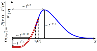
Figure 1: (Color online) A schematic representation of the scaling solution $G(x,t)$ (see Eq. (21)) at a given late time $t\gg 1$ (not drawn to scale). The red double line represents the small-$x$ scaling form $g(x/t^{1/(b+1)})t^{-\delta}$ while the blue solid line represents the large-$x$ scaling form $f(x/t^{1/2})t^{-\beta}$. The interval on which the two solutions overlap (Eq. (14)) is labeled $x_{1}(t)$.

Summarizing the results of the scaling analysis, we find that the solution of Eqs. (1)–(2) is, to leading order in $t$,

$$P(x,t)\approx P^{*}(x)+P^{*}(x)\cdot\left\{\begin{array}[]{ll}g\bigl{(}\frac{x}{t^{\gamma}}\bigr{)}t^{-\delta},&x\leq x_{1}(t)\\ \\ f\bigl{(}\frac{x}{t^{1/2}}\bigr{)}t^{-\beta},&x\geq x_{1}(t),\end{array}\right.,$$ (21)

where $f$ and $g$ are given in Eqs. (11) and (17), $\gamma$ and $\delta$ are given in (19), and $x_{1}(t)$ satisfies (14). We thus obtain a one-parameter family of scaling solutions parameterized by $\beta$. Below we denote a member of this family by $P_{\beta}(x,t)\equiv P^{*}(x)[1+G_{\beta}(x,t)]$. The overall form of these scaling solutions for $G$ is given schematically in Fig. 1. For small-$x$, the function is flat, with a value that approaches zero as $t^{-\delta}$. For $x\geq x_{1}(t)$, it exhibits a peak at $x\sim\sqrt{t}$, whose height scales as $t^{-\beta}$. Thus, as time progresses, the peak shrinks and moves to the right, and $G$ approaches its steady-state value $G(x,t\to\infty)=0$.

II.2 Selection mechanism

To conclude our analysis, we argue now that the parameter $\beta$ is selected by the tail of the initial distribution. To this end, we consider initial distributions of the form

$$G_{0}(x\gg 1)\sim Ax^{-a}$$ (22)

where $a>b-1$ and $A$ are parameters. Initial conditions $G_{0}(x)$ which decay faster than algebraically correspond to $a=\infty$. Note, however, that localized initial distributions $P(x,0)$ correspond to $a=0$. Since the dynamical process of Eq. (1) is diffusive, one would naively expect the tail of the distribution to remain unchanged for $x\gg\sqrt{t}$. Using the asymptotics (18), this suggests that $\beta=a/2$. The parameter $C$ is then given by $C=A/B$. Substituting the value of $B$ yields Abramowitz and Stegun (1972)

$$C=\frac{\Gamma(1-a/2)}{2^{1+b+a}\Gamma(\frac{3+b}{2})}\,A.$$ (23)

This naive argument is found to be valid only for $a<2$. For $a>2$ we make use of Eq. (8) to demonstrate that the correct scaling solution is given by $\beta=1$. This is done by analyzing the stability of a scaling solution with a given $\beta$. We thus consider a perturbation $\delta P(x,t)$ around the scaling solution (21):

$$P(x,t)-P^{*}(x)=P^{*}(x)G_{\beta}(x,t)+\delta P(x,t),$$ (24)

which is initially localized in $x$, such as a function with compact support. Normalization dictates that $\int\delta Pdx=0$. This perturbation satisfies Eqs. (1)–(2).

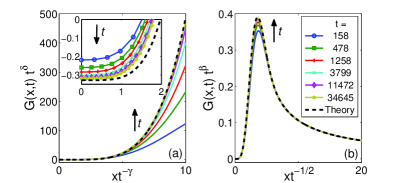
Figure 2: (Color online) The (a) small-$x$ and (b) large-$x$ scaling collapse obtained by numerically integrating Eq. (27) for $b=3.5$ and $a=1$. Different curves correspond to different times in increasing order in the arrow direction. The dashed curve is the theoretical function (21), with no fitting parameter. Inset shows a magnified region around the origin.

The scaling solution $G_{\beta}$ is stable to such perturbations and will dominate the approach to equilibrium only if at late times $\delta P(x,t)$ is negligible compared to it. The exact solution of Eq. (1) reveals that the scaling solution (8) to which a localized initial condition converges at long times is of the form (21) with $\beta=1$ Hirschberg et al. . This can be understood heuristically by noting that $\beta=1$ is the most localized of all scaling solutions, see (18). Therefore, the scaling form at large-$x$ of Eq. (24) is given by

$$P(x,t)-P^{*}(x)=P^{*}(x)G_{\beta}(x,t)+\delta P(x,t)\\ \approx P^{*}(x)\Bigl{[}t^{-\beta}f_{\beta}\Bigl{(}\frac{x}{\sqrt{t}}\Bigr{)}+t^{-1}f_{1}\Bigl{(}\frac{x}{\sqrt{t}}\Bigr{)}\Bigr{]},$$ (25)

where $f_{\beta}$ is the solution (17) corresponding to $\beta$. For $\beta<1$ the second term on the right-hand side is negligible compared to the first, and therefore the $f_{\beta}$ solution is stable. On the other hand, for $\beta>1$ the second term is dominant and the scaling solution is given by $f_{1}$. Thus,

$$\beta=\beta(a)=\left\{\begin{array}[]{ll}\frac{a}{2}&\text{if }a<2\\ 1&\text{if }a>2\end{array}\right..$$ (26)

The exact solution of the Fokker-Planck equation further reveals that when $a=2$ there are logarithmic corrections to Eq. (21) Hirschberg et al. . Note that for $a>2$, the constant $C$ is not given by (23) and it depends on the details of the initial condition. The large-$x$ scaling solution for localized initial distributions (corresponding to $a=0$) agrees with the results previously obtained in Godrèche and Luck (2001); Levine et al. (2005); Kessler and Barkai (2010). Knowledge of the scaling solution for other initial conditions is often required for calculating correlation functions of physical interest. Applications of this approach to physical examples where the late time behavior is determined by the initial conditions will be presented elsewhere Hirschberg et al. .

In order to check the applicability of the scaling solution found in this analysis, we studied numerically the evolution of a single-site zero-range process at criticality Evans and Hanney (2005). In this process, particles hop into a site with a constant rate 1, and hop out of this site with rate $w(n)=1+b/n$, where $n$ is the number of particles in the site. The occupation number probability distribution $P(n,t)$ satisfies the master equation

$$\frac{\partial}{\partial t}P(n)=P(n\!-\!1)+w(n\!+\!1)P(n\!+\!1)-[1+w(n)]P(n).$$ (27)

This is a discrete version of (1)–(2). Its steady state is given by $P^{*}(n)\propto[w(1)\ldots w(n)]^{-1}\sim n^{-b}$. We have studied the relaxation to the steady state starting from various initial conditions. In Fig. 2 we display the results obtained for an initial condition with $a=1$. A very good agreement with the predicted scaling functions is obtained at long times. To investigate the dependence (26) of the scaling exponents on the initial condition, we have measured $G(0,t)$ which is predicted to decay to zero as $t^{-\delta}$ (19). As an independent measure, we calculated $\langle n(t)\rangle$, which is predicted to decay to its equilibrium value $\langle n\rangle_{\text{eq}}$ as $t^{-\sigma}$ with $\sigma=\beta+b/2-1$. This can be easily obtained using the scaling function (21):

$$\langle n(t)\rangle-\langle n\rangle_{\text{eq}}\approx t^{-(\beta+b/2-1)}C\int_{0}^{\infty}u^{1-b}f(u)du.$$ (28)

In Fig. 3 we compare numerical measurements of $\delta$ and $\sigma$ to the theoretical predictions and find a very good agreement, both for $a<2$ and $a>2$.

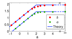
Figure 3: The scaling exponents $\delta$ and $\sigma$ obtained by numerical integration of (27), compared with theoretically predicted values. Here $b=2.9$ and $A=1$. The transition at $a=2$ is readily seen.

II.3 Other boundary conditions

The analysis presented above may be extended to consider other boundary conditions as well. For example, for an absorbing boundary condition at $x=0$, namely $P(0,t)=0$, the stationary distribution vanishes. Defining $G(x,t)$ by

$$P(x,t)=e^{-V(x)}G(x,t)$$ (29)

and repeating the derivation outlined above for the evolution of $G$, we find that in the scaling limit it takes the same form (12) as before, with $f$ unchanged, $\gamma=0$ and a different function $g(z)$ which can be calculated explicitly Hirschberg et al. . Equation (26), which yields the relation between $\beta$ and $a$, remains valid. However, since $G$ is defined differently in this case, the same initial distribution $P(x,0)$ would correspond to different values of $a$ depending on whether the boundary condition is reflecting or absorbing. Other boundary conditions, and the case where the equation is defined on the entire $x$-axis, may be treated similarly Hirschberg et al. .

III Conclusion

In summary, the approach to equilibrium of a diffusion process in a logarithmic potential is analyzed in the scaling limit and is shown to exhibit uncommon and interesting features. These include the existence of two characteristic length scales, the fact that the scaling function depends on the tail of the initial distribution, and the non-analytic way the scaling exponents varies with the initial condition. The mechanism by which the scaling exponents are selected is similar to the one encountered in problems of velocity selection in propagating fronts Barenblatt (1996); van Saarloos (2003). Here, however, unlike problems of front propagation, the evolution equation is linear, although inhomogeneous. This facilitates the explicit demonstration of the selection mechanism.